Article

Risk Evaluation Model of Coal Spontaneous Combustion Based on AEM-AHP-LSTM

1
College of Science, North China University of Science and Technology, Tangshan 063210, China
2
School of Mining Engineering, North China University of Science and Technology, Tangshan 063210, China
3
School of Economics, North China University of Science and Technology, Tangshan 063210, China
4
College of Yisheng, North China University of Science and Technology, Tangshan 063210, China
5
School of Basic Medical Sciences, North China University of Science and Technology, Tangshan 063210, China
*
Author to whom correspondence should be addressed.
Mathematics 2022, 10(20), 3796; https://doi.org/10.3390/math10203796
Submission received: 8 August 2022 / Revised: 26 September 2022 / Accepted: 3 October 2022 / Published: 14 October 2022
(This article belongs to the Special Issue Engineering Calculation and Data Modeling)

Abstract

:
Immediately and accurately assessing the risk of coal spontaneous combustion and taking targeted action are crucial steps in coal spontaneous combustion prevention and control. A new model, AEM-AHP-LSTM, was proposed to solve the weight calculation problem of multiobjective evaluation in the process of coal spontaneous combustion. Firstly, the key indicators of coal spontaneous combustion were analyzed and used as risk factors to establish an evaluation system. Next, the objective and subjective weights were calculated using AEM and AHP, respectively. The objective and subjective weights were then combined, and TOPSIS was used to calculate the score of the evaluation sample. Finally, the obtained evaluation samples were trained with the BP, RBF, and LSTM model to resolve the problem of model overdependence on historical data and achieve the auto-adapt adjustment of weight with data change. Additionally, data from 15 typical Chinese coal mines were applied to the model. The results indicate that, compared with the BP and RBF neural networks, the LSTM model has higher prediction accuracy, stronger generalization ability, and stronger practicability. The modeling and application findings show that the AEM-AHP-LSTM model was better appropriate for the risk assessment of coal spontaneous combustion. This method can potentially be further applied as reliable approach for the assessment of mine disaster risk.

1. Introduction

One of the five enduring disasters in the world [1], the underground coal fire disaster, is also the biggest threat to coal mine safety production, severely impeding the safe expansion of the coal mine industry. Coal spontaneous combustion accounts for around 90% of the causes of underground mine fire disasters in China [2]. Once the coal spontaneous combustion disaster occurs, it will cause many hazards, such as waste of coal resources, damage to the environment, safety accidents, deterioration of ecology, damage to water bodies, and damage to people’s lives and health. These hazards seriously hinder the mining of coal, making the normal production of the mine impossible.
Therefore, it has always been crucial for mine safety production to find a solution to the problem of coal spontaneous combustion [3]. Immediately and accurately assessing the risk of coal spontaneous combustion and taking targeted action are crucial steps in coal spontaneous combustion prevention and control.
Coal spontaneous combustion is a highly dynamic, physical, and chemical transformation [4]. Indicators undergo a lot of modifications during this procedure. The main indicators that influence spontaneous combustion are those related to the inherent properties of coal, distinctive gas concentrations, and alterations in the environment. Experts and scholars domestically and internationally have carried out a lot of research on the risk of spontaneous combustion of coal.
Pattanaik et al. [5] performed chemical analysis, crossing point temperature (CPT), petrography, infrared studies (IR), and differential thermal analysis (DTA) tests on coal. A strong correlation between coal’s inherent characteristics and its propensity for spontaneous combustion was discovered. Ren et al. [6] developed an early warning indicators system for coal spontaneous combustion and divided the stages of spontaneous combustion of coal. The changing curve of the marker gas during coal spontaneous combustion was fitted using the logistic function. Statistical characteristics were used to calculate the parameter values. Zhang et al. [7] compared the heat flux and kinetic parameters before and after the CAIT. The effects of temperature increase rate and oxygen concentration on coal spontaneous combustion were discovered by TG/DSC analysis and mathematical model construction. By using the energy equation to create a better model, Lin et al. [2] established the model and provided an explanation of the mechanism by which temperature impacts coal spontaneous combustion.
However, traditional algorithms struggle to appropriately assess the danger because of the nonlinear relationship between indicators and coal spontaneous combustion. Current research has shifted its attention to how to develop a technique for reliably assessing the risk of spontaneous combustion. Numerous research technologies have been proposed by researchers to evaluate the risk of coal spontaneous combustion. These include AEM-TOPSIS [8], variable weight gray model [9], G1 combined weighted cloud [10], analytic hierarchy process [11], entropy weight extension evaluation method [12], Bayesian network [13], game extension method [14], neural network [15,16], random forest [3,17,18], support vector machine [19,20,21,22], and G2-TOPSIS [23].
Xing et al. [8] used the anti-entropy weight method to calculate the evaluation index’s weight. Based on TOPSIS, a model for assessing the danger of coal spontaneous combustion was created. The model was used to simulate the coal mining face of a typical Chinese coal mine. Xu et al. [9] conducted a simulated spontaneous combustion test of programmed heating coal. The gray target theory and gray entropy correlation analysis method were used. A variable weight-based gray target algorithm was established to quantitatively evaluate the risk of spontaneous combustion. In order to determine the risk of coal mine spontaneous combustion, Su et al. [10] examined the factors of spontaneous combustion from three perspectives: coal spontaneous combustion tendency, air leakage and oxygen supply, and heat storage and heat dissipation, and a COWA-modified G1 combined weighted cloud model was proposed.
Wang et al. [11] used the AHP method to calculate the index weights, and extended the set pair theory. A coal spontaneous combustion risk analysis model was constructed to determine uncertain information. The results showed that the model analysis process was reasonable and had high confidence. Wang et al. [12] used the entropy weight method to establish an entropy weight extension comprehensive evaluation model. The data of the spontaneous combustion were used to verify the model. The results obtained by this method were in line with the actual situation. Zhang et al. [13] combined qualitative analysis with quantitative analysis based on Bayesian network, and HAZOP-LOPA (analytic hierarchy process) of protection of coal mine safety risk was proposed.
Han et al. [14] proposed a game extension algorithm that used game theory to combine the subjective and objective weight analysis with the extension tendency analysis. The state of the evaluation object, the development trend of the state, the subjective weights, and objective weights can be obtained by the algorithm. Based on this, the evaluation level of each evaluation object was obtained to describe the development trend of the index. Xu et al. [15] employed the neural network method to forecast the coal spontaneous combustion’s limit parameters. The outcomes demonstrated that artificial neural networks were better suited to handle such challenging issues in underground mines. Li et al. [16] proposed a method for predicting and risk assessment of gas gushing in a fully mechanized mining face based on LSTM. The adaptive moment estimation optimization algorithm was used to optimize the parameters in the model through first-order deviation and second-order deviation correction. The mean square error (MSE) was selected for use as the evaluation index of the model. It was finally found that the risk assessment error of the LSTM neural network was smaller, the prediction value was more accurate, and it had better practical value.
Deng [3], Matin [17], and Chelgani [18] applied the random forest algorithm to the modeling analysis of coal spontaneous combustion prediction, coal calorific value estimation, and coal free swell index (FSI) in gobs, respectively. The results showed that the random forest algorithm had good performance in the coal field. Ma [19], Wang [20], and Deng [21,22] used genetic algorithm, rough set, particle swarm algorithm, and support vector machine to solve the problem of risk prediction in the process of spontaneous combustion of coal.
Wei Wang et al. [23] proposed an improved CRITIC-G2-TOPSIS dynamic model. The model improved criterion importance through intercriteria correlation (CRITIC) and modified the technique for order of preference by similarity. The results demonstrated to be scientific in predicting the goaf spontaneous combustion risk. The model had important popularization and application value.
Many indicators related to coal spontaneous combustion are difficult to quantify by traditional methods [24]. The index assignments that affect coal spontaneous combustion vary greatly. Therefore, attention should be paid to the differences between the indicators. At the same time, the current methods of evaluating weights are either too subjective or too objective. Additionally, the evaluation results are overly reliant on historical data, and it is difficult to apply different index values to various local mines.
To resolve the aforementioned issues, the AEM-AHP-LSTM model is proposed. The index system of coal spontaneous combustion risk variables is adopted after analyzing the inherent properties of coal, the impact of hallmark gas concentrations, and changes in the environment. The AEM-AHP-LSTM model is proposed to create a new combination evaluation algorithm, which is tested using data from various common coal mines in China. The proposed model can effectively estimate the likelihood and propensity of coal spontaneous combustion in a coal mine, enhance mine intelligence, and maximize resource utilization.

2. Methods

2.1. Anti-Entropy Method

The anti-entropy method (AEM) is an improved algorithm based on the entropy weight method (EWM) [8]. The method is used to solve the sensitivity of the differences between the entropy weight method indicators. Individual weights are abnormal in the weight distribution because the weight calculated by EMW is more sensitive to the index difference. Both AEM and EWM are objective weighting methods that do not include any subjective elements and rely heavily on the features revealed by the data. The fundamental difference between AEM and EWM is that AEM uses anti-entropy instead of entropy as its measure of entropy. The following are the key steps:
Step 1. Create the initial data matrix. A matrix of the evaluation matrix X can be obtained with m indicators and n evaluation objects. X is standardized.
X = x 11 x 1 n x m 1 x m n
Step 2. Calculate the anti-entropy value of each indicator E i j and the weights w j
E j = i = 1 m P i j ln 1 P i j
where P i j = X i j / i = 1 m X i j
w j = E j / j = 1 n E j

2.2. Analytic Hierarchy Process

The analytic hierarchy process (AHP) is a widely used decision-making method that provides qualitative and quantitative analysis [25]. It is a method for subjectively calculating weights to indicators. The quantitative evaluation of indicators heavily relies on the experience of decision-makers. AHP is so subjective that it cannot expose the information in the data. AHP depends heavily on experts’ expertise of the evaluated objects to calculate the weights of assessment indicators. The key steps are as follows:
Step 1. Establish judgment matrix using the nine-scale evaluation scale for the indicators at the criterion level and the scheme level. The importance scaling approach is used to compare the indicators of the same layer in pairs, and values between 1 and 9 are chosen to create the judgment matrix A.
A = a 11 a 12 a 1 n a 21 a 22 a 2 n a n 1 a n 2 a n n n × n
where m is the number of evaluation indicators, and a i j represents the relative importance degree between the evaluation indicators.
Step 2. The consistency test is carried out. Calculate the ratio of the consistency index CI to the average random consistency index RI. The value of RI is shown in Table 1. Obtain the consistency ratio CR, and based on this, judge whether the consistency of the matrix A is acceptable.
CR = CI / RI
CI = λ max m / ( m 1 )
where λ max is the largest eigenvalue of the judgment matrix A.
Step 3. Use the geometric mean method and the normalization method to calculate the subjective weight of the evaluation index.
v i = j = 1 m a i j 1 m i = 1 m j = 1 m a i j 1 m , i = 1 , 2 , m

2.3. Comprehensive Weight

Combined weight includes both subjective information and objective information.The principle of minimum information discrimination is used to calculate combined weight [26]. The weight obtained by the subjective weighting approach is too subjective. The weight obtained by the objective weighting method is overly biased in favor of the data. This method aims to overcome these issues.
min F = j = 1 n w j ln w j w a j + j = 1 n w j ln w j w b j s . t . j = 1 n w j = 1 ; w j > 0
The Lagrange multiplier is introduced to solve the above formula, and the calculation formula of the comprehensive weight is obtained as follows:
X j = w j v j j = 1 n w j v j

2.4. TOPSIS

TOPSIS is the approximation to the ideal ranking method, which is a comprehensive index evaluation method [23]. Each sample’s proximity to the comparison sequence is calculated to assess the evaluation. Proximity comprises the best and worst values of each index across all samples. TOPSIS is a way to explain the overall impact of many indicators. The distribution of the data, sample size, and indicators are not subject to any tight limitations. It is appropriate for both big systems with numerous samples and indicators and small sample data. It is more practical and versatile. Additionally, it has limited data sensitivity. The following are the key steps.
Step 1. Establish the original data matrix and standardize it, set the object set as P = { P 1 , P 2 , , P m } , and set the object evaluation index as r = { r 1 , r 2 , , r n } . Then, the original data matrix is
P = r i j m × n = r 11 r 12 r 1 n r 21 r 22 r 2 n r m 1 r m 2 r m n
Y a b + = r a b min ( r i j ) max ( r i j ) min ( r i j ) , positive indicator
Y a b = max ( r i j ) r i j max ( r i j ) min r i j , negative indicator
Step 2. Calculate the positive and negative ideal solutions, and the score.
Y + = max Y i j i = 1 , 2 , 3 , , a = Y 1 + , Y 2 + , , Y b +
Y = min i j i = 1 , 2 , 3 , , a = Y 1 , Y 2 , , Y b
Step 3. Define the distance between the i-th evaluation index and the maximum value, as follows.
D i + = j = 1 m ω j Z j + z i j 2
Define the distance between the i-th evaluation index and the minimum value as
D i = j = 1 m ω j Z j z i j 2
Calculate the score as
S i = D i D i + + D i

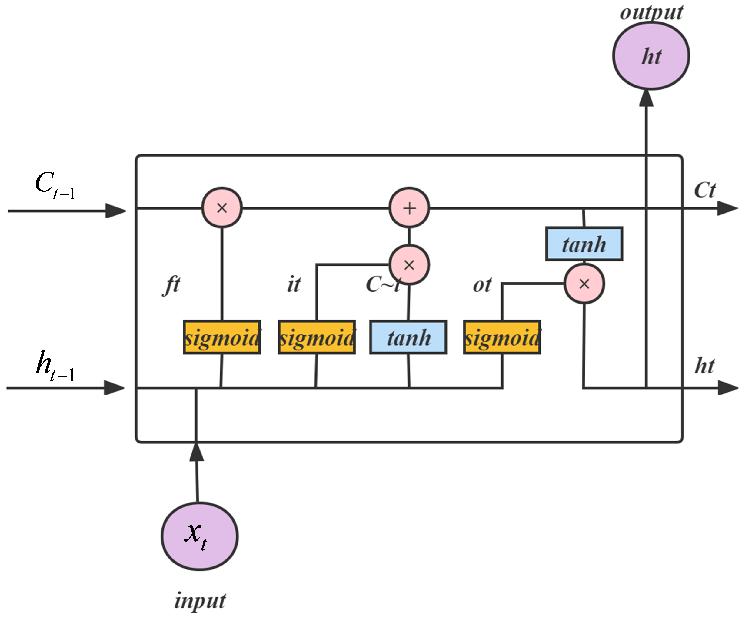
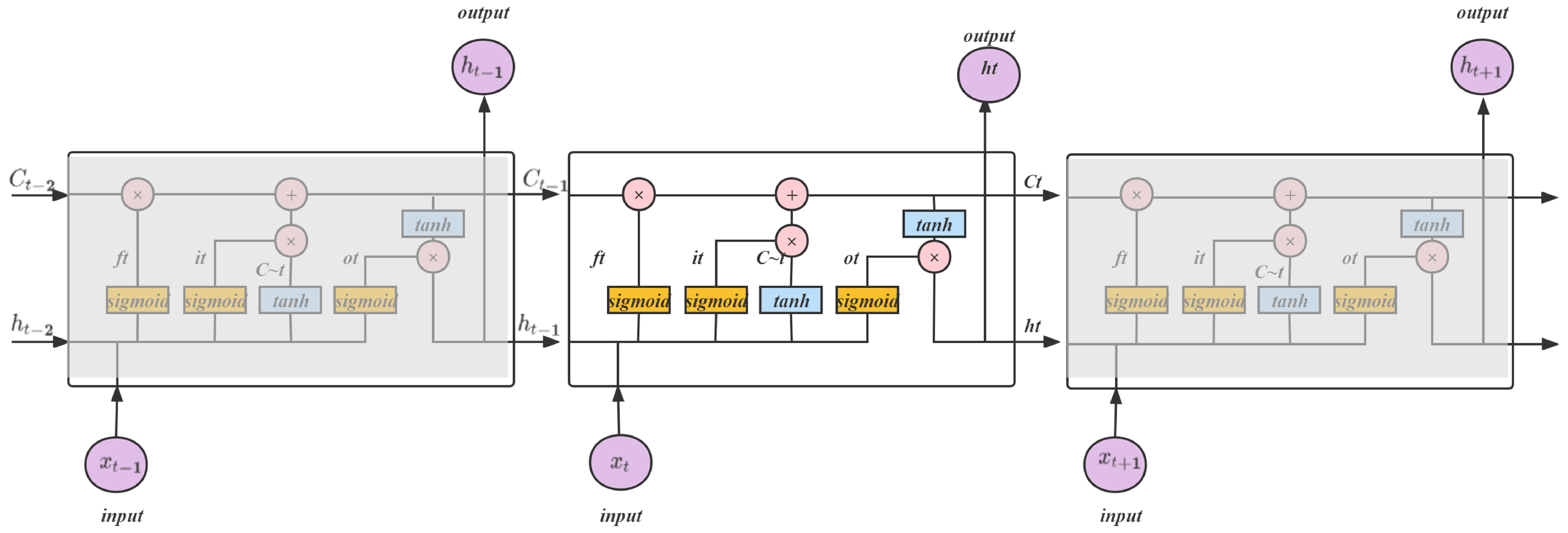
2.5. Long Short-Term Memory Neural Network

The long short-term memory neural network (LSTM) is a variant of recurrent neural network (RNN) [27]. LSTM primarily addresses the issue of “gradient explosion” or “gradient disappearance” when training long sequences. The issue results in the weight of the neural network training being obtained during the backpropagation process. Three gate mechanisms and an extra cell unit are added to LSTM in comparison to RNN.
The fundamental component of LSTM is the unit state, which is the horizontal line of the upper series unit in Figure 1. With only a few linear interactions, the entire cell state behaves similar to a conveyor belt moving through the complete LSTM chain system. The data can remain unmodified as they move through the structure.
The activation function of the LSTM’s basic unit model and the data output transfer between each neuron are used to finish the prediction process (in Figure 2). The forget gate, input gate, and output gate are the three gates that regulate the unit state features of the structure in the LSTM model with three unit gates.
Forget gate: The forget gate’s sigmoid layer is used by the LSTM to assess whether or not to forget the data that have to be removed from the unit state. The data of this sequence and the hidden state of the prior sequence are produced by the forget gate as a vector from 0 to 1, where 1 denotes the complete retention of all data, while 0 denotes its complete deletion. The following is the gate’s precise formula:
f t = σ W f · h t 1 , x t + b f
where h t 1 is the output information when t − 1, x t is the input information of this layer when t, W f is the weight of each variable, b f is the intercept term, and the value of f t is from 0 to 1. σ is the sigmoid function, and the formula of the sigmoid function is
σ ( x ) = ( 1 + e x ) 1
Input gate: Information is determined after the forgetting process by the forgetting gate is complete. Then, the new data need to be added to the United States. There are two steps in this process. Use h t 1 and X t to determine which information needs to be updated by the sigmoid layer. The new candidate cell state is then discovered using tanh. This data information can now be changed to a single state. The following is the gate’s precise formula:
i t = σ W i · h t 1 , x t + b i
C ˜ t = tanh W c · h t 1 , x t + b c
where tanh is the tangent activation function, and C ˜ t represents the information to be recorded from the input information of time t.
After that, the old unit state C t 1 is updated to the new unit state C t . The detailed process of this part is to multiply the results of the old unit state and the forgetting gate, then add new input data information to the current unit state. In this way, some old information will no longer be used.
C t 1 represents the unit state value at t − 1, and C t is the refreshed unit state value.
Output gate: The state characteristics of the output unit must be established using the updated unit state sum of the input once the unit state has been updated. To decide how much information needs to be output, the sigmoid layer of the output gate must evaluate the incoming data. The output value of the tangent activation function, tanh, is then obtained from the unit state C t . The final output is taken to be the judgment condition that was obtained by multiplying the vector by the output gate.
o t = σ W o · h t 1 , x t + b o
h t = o t · tanh C t
The internal architecture of a single neuron is made possible by the processing mechanism of these three gates. The architecture enables the LSTM model to effectively create a data memory for incoming data coming from a distance.

2.6. Model Performance Evaluation Metrics

Mean absolute error (MAE), mean absolute percentage error (MAPE), root mean square error (RMSE), and coefficient of determination R 2 are measures used to assess the performance of models [28,29]. RMSE, MAE, and MAPE are used to evaluate the regression results of the LSTM model. The RMSE, MAE, and MAPE calculation formulas are as follows.
RMSE = 1 n i = 1 n f i y i 2
MAE = 1 n i = 1 n f i y i
MAPE = 1 n i = 1 n f i y i y i × 100 %
MSE = 1 n i = 1 n Y i Y ^ i 2

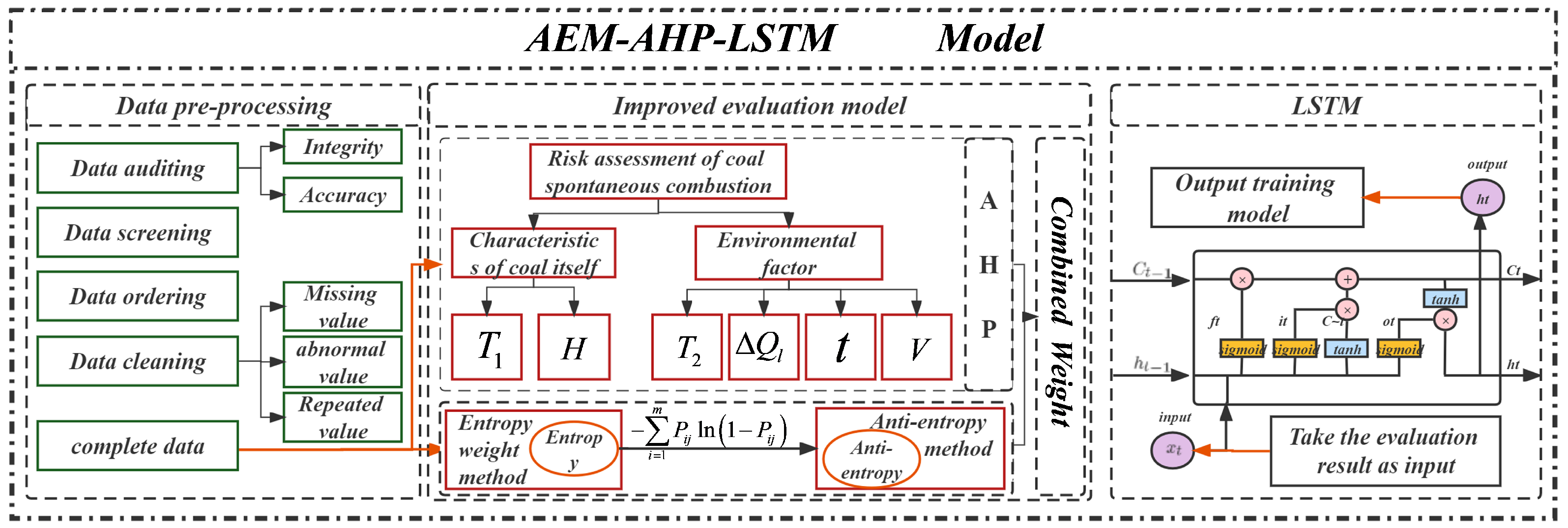
2.7. AEM-AHP-LSTM Model

In order to obtain better training accuracy, the data should be preprocessed before training the model. The primary steps include data screening, data sorting, data cleaning, and data accuracy and completeness review. Missing numbers and outliers in the data are removed throughout the cleaning process. Additionally, duplicate values are handled and typically eliminated. The model can begin to be trained after the data are prepared.
The algorithm steps are as flows:
Step 1. Initialize the data. Construct the original data matrix and standardize the data:
y = x μ σ
Step 2. Calculate the anti-entropy and calculate the objective weight:
w j = E j / j = 1 n E j
Step 3. Construct the judgment matrix, check its consistency, and calculate the subjective weight:
v i = j = 1 m a i j 1 m i = 1 m j = 1 m a i j 1 m , i = 1 , 2 , m
Step 4. Calculate the comprehensive weight:
ω j = w j v j j = 1 n w j v j
Step 5. Forward the original data matrix, and calculate the positive and negative ideal solutions.
Step 6. Calculate the distance from the ith index to the maximum and minimum values, and the score.
Step 7. Take the original data as the inputs and the score as the outputs. Divide the dataset: 70% as the training set and 30% as the validation set.
Step 8. Train the LSTM model and validate the model with 30% of the validation set.
Step 9. Output the model performance indicators RMSE value, MAE value, MAPE value, and the score of each sample.
The majority of the traditional evaluation models’ weighting procedures rely heavily and arbitrary on data. To improve the current situation, the subjective weighting methods and objective weighting methods are combined to counter entropy weights. The calculation formula for the comprehensive weight is finally discovered, and the comprehensive weight is obtained. The minimum identification information is used as the objective function. The weight sum is 1 and the weight is greater than 0 as a constraint. To determine the score of each mine, TOPSIS is used to score each sample after collecting the weight. The mine is subject to a single danger, according to the data analysis. Factor flaws assist mines in lowering the probability of coal spontaneous combustion.
The LSTM regression model is created to make the AEM-AHP model trained and packed. Each evaluation model index is the dependent variable, and the final score is the independent variable. The goal of LSTM is to make weight computation simpler, and increase the model operation speed so that the developed model can be used to estimate risk for other mines and is more suited to the real-world scenario of engineering calculations. The LSTM model can create its own weight for each sample, allowing it to adaptively calculate each sample’s score. Figure 3 depicts the model’s overall concept.

3. Experimental Simulation

3.1. Indicator Selection

The physical and chemical changes that occur during the spontaneous combustion of coal are extremely complicated, dynamic, and challenging to define [30,31]. The indicator system is based on the analysis of numerous statistical data and the pertinent literature. Indicators are the amount of air leakage at the working face, the amount of time the oxidation zone has access to continuous oxygen supply, the thickness of the floating coal, the temperature of the nearby rock, and the rate at which the working face is moving forward. The indications and their symbols are described as follows.
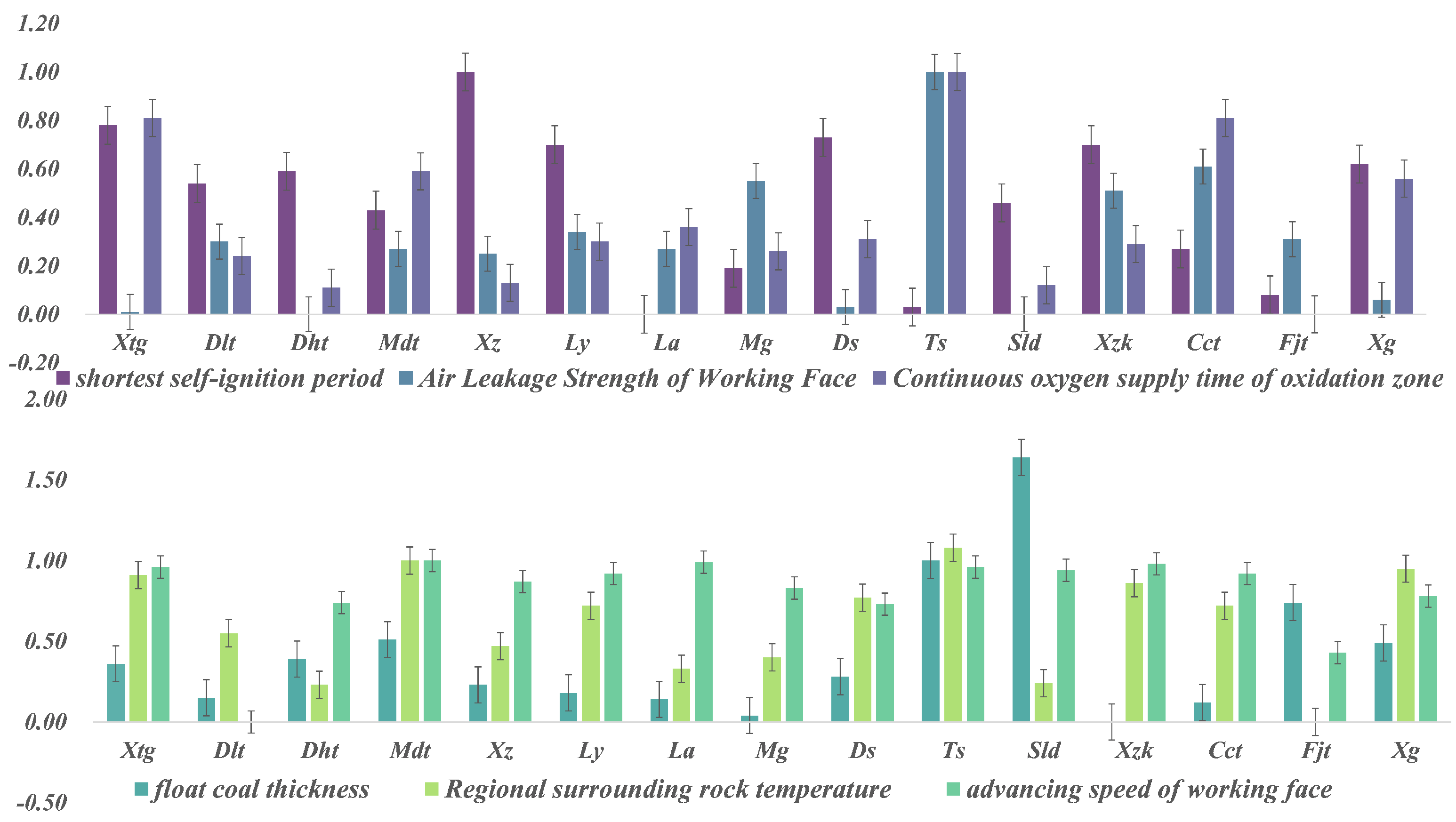
  • The shortest spontaneous ignition period ( T 1 ): The minimum time required for coal to spontaneously combust from mining. The index is an intuitive index to reflect the strength of thermal effect in the process of coal spontaneous combustion, and it is also an important parameter to evaluate the risk of coal spontaneous combustion. The shorter the time, the greater the possibility of spontaneous combustion [32,33].
  • Air leakage intensity of working face ( Δ Q l ): The working face’s air leakage intensity is influenced by a number of variables, including the air intake volume, working face length, mining height, etc. To calculate the impact of spontaneous combustion, the air leakage intensity is multiplied by the air leakage speed. This index is an important characterization index showing the spontaneous combustion tendency of coal [34,35].
    Δ Q l = 4 · Q a Q b L · H Q a + Q b 2 · Q 2
    where D e l t a Q l is the air leakage intensity of the working face, Q a , Q b are the measured inlet air volume and return air volume of the mining face, respectively, H is the length of the working face and the mining height, and Q is the air supply volume of the mining face.
  • Oxidation zone continuous oxygen supply time ( T 2 ): The likelihood of spontaneous combustion in the goaf depends on the duration of continuous oxygen delivery in the oxidation zone. The likelihood of spontaneous combustion increases with the duration of continuous oxygen supply. The longer the continuous oxygen supply, the greater the possibility of spontaneous combustion [36,37].
  • Thickness of floating coal (H): The substance that supports spontaneous combustion is the thickness of floating coal. The amount of heat emitted by the oxidation reaction and the likelihood of spontaneous combustion increase in direct proportion to the thickness of the floating coal pile. The greater the thickness of the floating coal accumulation, the greater the probability of spontaneous combustion [38].
    H = K H c ( 1 α ) + M M 1 ( 1 β ) + m 1 + m 2
    H 1 = K M ( 1 α ) + m 1
    where H is the top coal caving mining, H 1 is the floating coal thickness of the full height goaf in primary mining, K is the coal loosening coefficient, which is taken as 1.5, M is the coal seam thickness, m 1 is the cumulative thickness of the non-minable coal seam within the upper caving range, and m 2 is the estimated thickness of the remaining coal in the upper old gob.
  • Regional surrounding rock temperature (t): The region’s increased rock temperature will raise the coal’s oxidation activity, speed up the reaction process, and release a significant quantity of heat, which creates an ideal setting for storing heat for spontaneous combustion. The higher the temperature of the surrounding rock in the area, the greater the risk of spontaneous combustion [39].
  • Working face advancing speed (V): The likelihood of spontaneous combustion of coal is reduced by shorter working face advancement times, shorter continuous fixed-point air leakage times, shorter continuous oxygen supply conditions in the oxidation zone, and shorter working face advancement times. The greater the working face advancing speed, the greater the risk of spontaneous combustion [40].

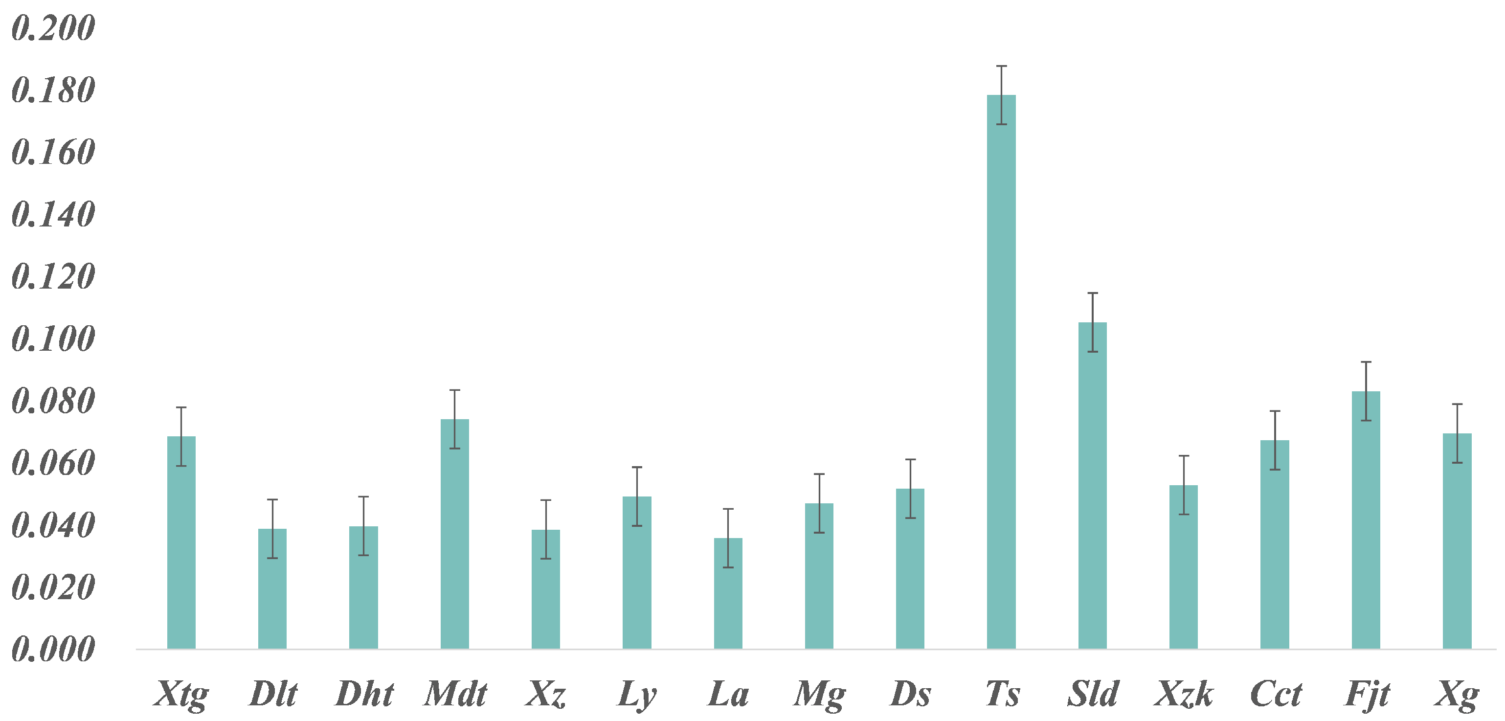
3.2. Data Source and Preprocessing

The model is trained using the risk assessment data for coal spontaneous combustion. The data are from 15 typical domestic coal mines that were taken from the relevant literature and actual production. The air leakage intensity of the working face, the continuous oxygen supply time of the oxidation zone, the thickness of floating coal, and the temperature of the surrounding rock in the area are positively correlated with the risk level of spontaneous combustion. Firstly, the data are evaluated, filtered, and sorted in order to assess their completeness, repeatability, and timeliness. Next, the suitability of the data for the model is assessed. The information is then cleaned, duplicate values are eliminated, and missing values are filled in using interpolation. Finally, the data are normalized to remove the impact of dimensions, making the data of each indicator comparable, and the final data are displayed in Figure 4.
The data in this paper are the float data of 15 samples of 6 indicators, and the detailed data are shown in Figure 4. It can be seen from the figure that the characteristics presented by the data of different samples are different. Generally speaking, the value of air leaking strength of working face is small, and this indicator is a maximum value indicator. Therefore, coal mines should pay attention to the prevention of the indicator and take corresponding measures to prevent and control the possibility of spontaneous coal combustion. The results of descriptive statistical analysis of the data in this paper are shown in Table 2.

3.3. Results and Discussion

Bringing the data into Formula (5) in the AEM model, the anti-entropy E j is obtained as follows:
E j = 0.0970 , 0.1304 , 0.1089 , 0.1478 , 0.0883 , 0.0764 T
The weights derived from AEM are
w j = 0.1494 0.2010 0.1678 0.2278 0.1361 0.1178 T
We enter the following judgment matrix for AHP to calculate the weights.
1 4 2 1 1 4 1 / 4 1 1 / 2 1 / 4 1 / 4 1 1 / 2 2 1 1 / 2 1 / 2 2 1 4 2 1 1 4 1 4 2 1 1 4 1 / 4 1 1 / 2 1 / 4 1 / 4 1
The weights calculated by AHP are
v j = 0.25 0.0625 0.125 0.25 0.25 0.0625 T
Finally, the weight obtained by the combined weighting is
W j = 0.221 0.074 0.124 0.337 0.201 0.043 T
Taking the combined weight as the parameter of the TOPSIS model, the score of each mine is calculated as follows:
X =   [ 0.069 0.039 0.040 0.074 0.039 0.049 0.036 0.047 0.052 0.178 0.105 0.053 0.067 0.083 0.070 ] T
The TOPSIS model finally obtains the score data of each mine, as shown in Figure 5.
Different risk factors are the reflection of various risks associated with coal spontaneous combustion. As shown in Figure 5, the coal spontaneous combustion risk score of Ts is 0.178, which indicates that Ts has the largest risk of coal spontaneous combustion. According to Figure 4, the reason for the greatest risk of Ts is that the values of the four indicators are the largest. The four indicators are the working face’s air leakage intensity, the oxidation zone’s continuous oxygen supply time, the thickness of the floating coal, and the local rock’s temperature. The mine should focus on these four aspects, propose targeted treatment measures, and achieve hierarchical control.
The coal spontaneous combustion risk scores of Mdt, Fjt, and Sld are 0.074, 0.083, and 0.105, respectively. Mg, Ly, Ds, Xzk, Cct, Xtg, and Xg are the medium risk area. Greater risk exists for Sld, Fjt, and Mdt compared with Mg, Ly, Ds, Xzk, Cct, Xtg, and Xg; therefore, it is imperative to properly explore any potential threats. According to Figure 4, the air leakage intensity of the working face, the continuous oxygen supply time of the oxidation zone, and the temperature of the surrounding rock in the area are relatively low—and these are three indicators that should be paid attention to. La, Xz, Dlt, and Dht are the low-risk areas, as shown in Figure 5—their scores are 0.036, 0.039, 0.039, and 0.04, respectively. To lower the risk of coal spontaneous combustion, they should propose thorough preventative and control procedures. These results are consistent with reality.
The cause of the functioning face’s sluggish advancement must be discovered. From this perspective, it is possible to limit accidents and lower the risk of coal spontaneous combustion. Production safety is ensured by the potential of occurrence.

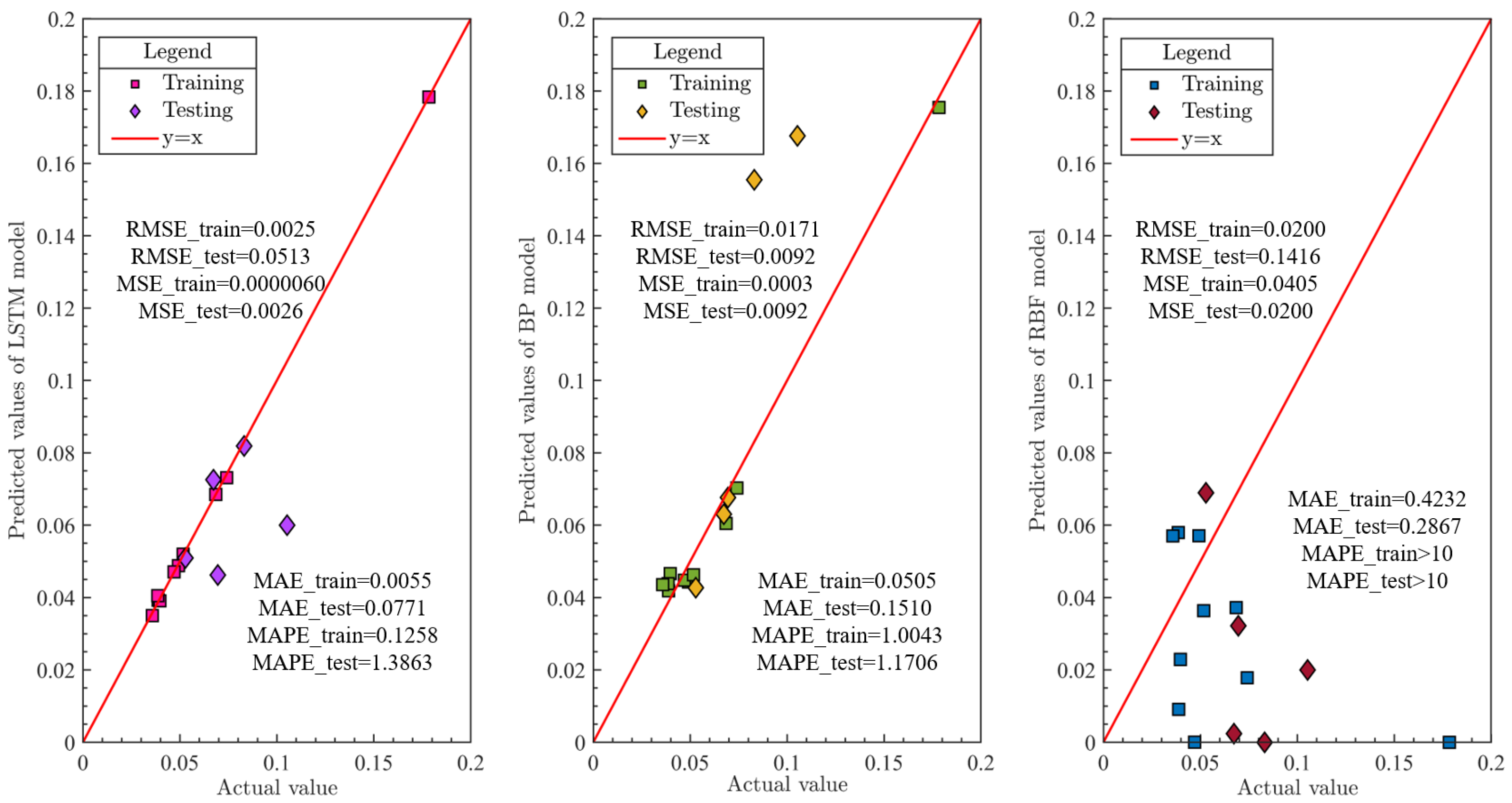
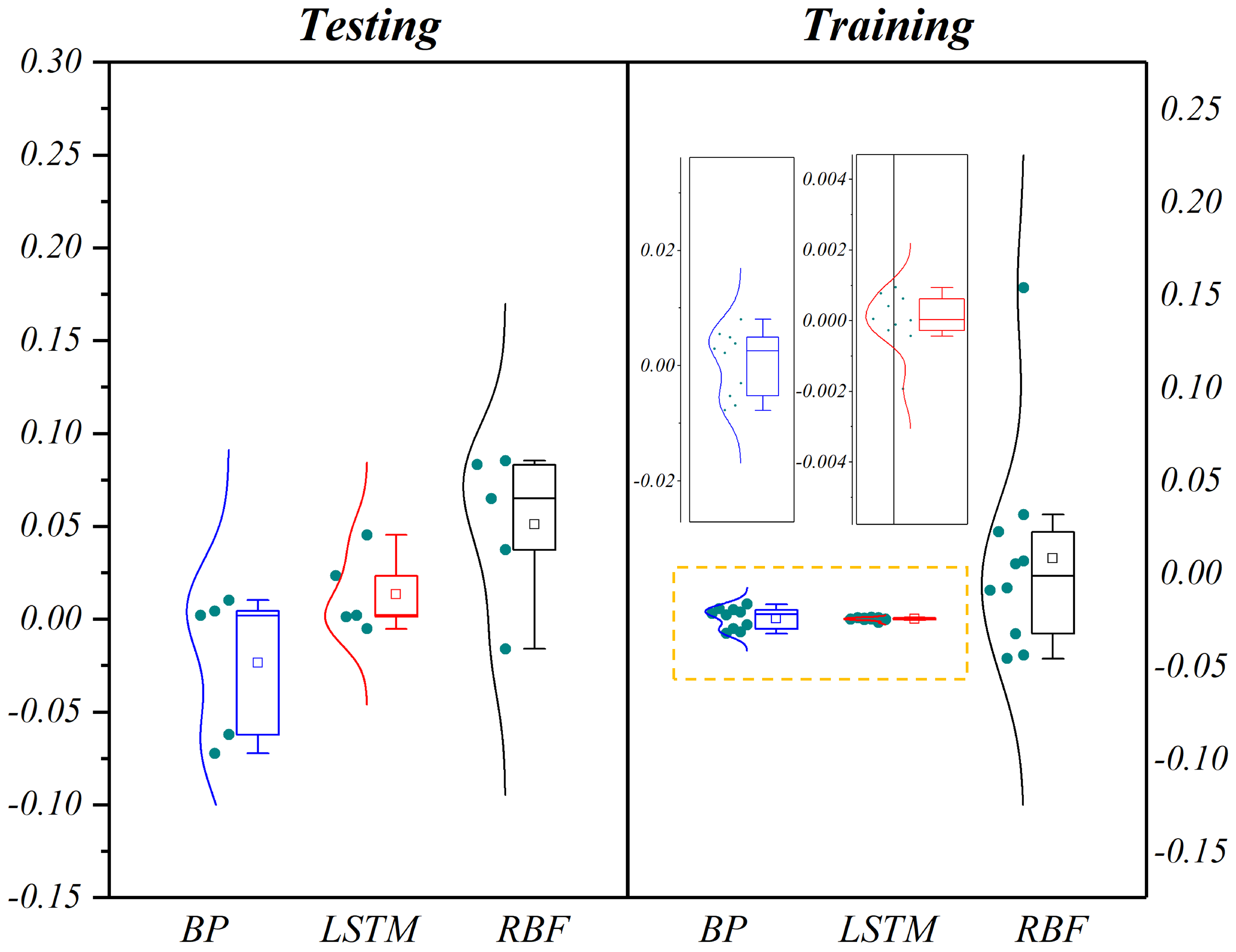
3.4. Prediction and Validation of Coal Spontaneous Combustion

LSTM modifies each index’s weight in accordance with the various samples, which speeds up computation time and simplifies the weight calculation process. It establishes the adaptive weight of each sample, which guarantees the model’s accuracy. In order to generate new sample results and shorten the running time, LSTM increases the model’s access environment to unexplored scenarios.
In addition, BP neural network and RBF neural network are used to predict the possibility of coal spontaneous combustion. The results of model training and prediction are shown in Figure 6, which shows the predicted features of the three models’ true values and predicted values. It can be seen from the figure that the predicted results are in good agreement with the actual results, which indicates that the prediction effects of the three models are all good. However, the prediction results of the BP neural network and the RBF neural network are relatively deviated from the y = x line, indicating that the generalization ability of these two models is not as good as that of the LSTM model. This conclusion can be further observed in the absolute error of Figure 7.
To further quantify and compare the performance of the three models, the evaluation index results of the three models are shown in Table 3. It can be seen from the data in the table that the effects of the three models are all good (RMSE < 0.2, MSE < 0.05, MAE < 0.5, MAPE < 3.5). The results of the LSTM model are better than those of the BP and RBF models. Compared with the BP and RBF neural networks, the LSTM model has higher prediction accuracy, stronger generalization ability, and stronger practicability, which indicates that the AEM-AHP-LSTM model proposed in this paper is more suitable for the prediction of spontaneous combustion of coal, and the model has a very broad application prospect.
MSE, MAE, RMSE, and other indicators can judge the quality of the model, but the difference in predictions between the two models may not be noticeable. Therefore, these model evaluation indicators alone cannot fully explain the quality of the model results. In response to this problem, Diebold and Mariano proposed the DM statistic to detect the difference in the predictive ability of different models. The DM test does not have the problem of autocorrelation and does not require the prediction error to satisfy a normal distribution with 0 means. Therefore, the DM test is used to test whether the difference in the prediction results between LSTM, BP, and RBF is obvious. The main idea of the DM test is to judge the difference between two models by constructing DM statistics. The DM statistic is given by Equation (41).
D M = S T ( T + 1 ) 4 T ( T + 1 ) ( 2 T + 1 ) 24 N ( 0 , 1 )
where rank d t   I + d t = 1 , d t > 0 = 0 , d t < 0 is the indicator function, and rank d t is the absolute value of the difference sequence of the corresponding loss functions of the two models.
The DM test results show that the DM value of LSTM and BP comparison is 0.7871. The DM value of LSTM and RBF comparison is 0.8483, and the DM value of BP and RBF comparison is 0.8603. The results all show DM value greater than 0.5, indicating that the differences between the models are obvious. The results show that on the test set, the effect of LSTM is better than that of BP, the effect of LSTM is better than that of RBF, and the effect of BP is better than that of RBF. Generally speaking, the model performance ranking is LSTM > BP > RBF.

4. Conclusions

In this study, an AEM-AHP-LSTM model was proposed to solve the weight calculation problem of multiobjective evaluation in the process of coal spontaneous combustion. This model achieved the auto-adapt adjustment of weight with data change. The data of 15 typical coal mines in China were used to simulate the model. Moreover, the BP neural network and SVM methods were adopted to compare with the presented RF model. The conclusions obtained are as follows:
(1) Compared with the previous study, a similar indicator system was selected. Based on the historical data of these indicators, an AEM-AHP model was established. The combination of AHP and AEM can solve the problem that some indicators in the previous coal spontaneous combustion evaluation methods cannot be quantified, and can greatly reduce the judgment errors caused by both subjective and objective aspects. The results of the AEM-AHP model were consistent with the actual situation. The model can help managers to judge and compare the risk of spontaneous combustion in different coal mines and take preventive measures for spontaneous combustion.
(2) The data were used as the LSTM model input to eliminate the previous study’s overdependence on historical data. A comparison between LSTM, BP, and RBF models revealed that the LSTM model achieved great predictive performance (MAE < 0.75, MAPE < 1%, RMSE < 0.01). The nonlinear fitting ability of the RBF model to the coal spontaneous combustion risk assessment data is poor. The results indicate that the LSTM model possesses strong generalization capacity with stability and applicability.
(3) The model proposed in this paper effectively solves the coal spontaneous combustion risk assessment problems and provides a certain theoretical basis for coal spontaneous combustion prevention. The validity of the method in this paper can be verified by mine safety risk investigation activities. To continue and expand around the application of the model in the field of coal processing, future work can be carried out on other important factors (mine safety production, mine hazard risk discovery).

Author Contributions

Investigation, X.Z., S.R., S.Z., J.Z. and Y.W. All authors have read and agreed to the published version of the manuscript.

Funding

This research was funded by Basic Scientific Research Business Fees for Provincial Colleges and Universities in Hebei Province: JQN2021011, Postgraduate Innovation Project of North China University of Science and Technology: CXZZBS2021102, and Innovation and Entrepreneurship Project of North China University of Science and Technology: X2022050.

Institutional Review Board Statement

Not applicable.

Informed Consent Statement

Not applicable.

Data Availability Statement

All data generated or analyzed during this study are included in this published article.

Acknowledgments

The authors are thankful to the editor and anonymous referees for their valuable comments and suggestions.

Conflicts of Interest

The authors declare no conflict of interest.

References

  1. Zhong, X.; Tang, Y.; Tian, X. The extraction and conversion method of thermal energy in large-scale coal field fire area. Coal Mine Saf. 2016, 10, 161–164. [Google Scholar]
  2. Lin, Q.; Wang, S.; Liang, Y.; Song, S.; Ren, T. Analytical Prediction of Coal Spontaneous Combustion Tendency: Velocity Range with High Possibility of Self-Ignition. Fuel Process. Technol. 2017, 159, 38–47. [Google Scholar] [CrossRef]
  3. Deng, J.; Lei, C.; Cao, K.; Ma, L.; Wang, C.; Zhai, X. Random Forest Method for Coal Spontaneous Combustion Prediction in Gobs. J. China Coal Soc. 2018, 10, 2800–2808. [Google Scholar]
  4. Gao, D.; Guo, L.; Wang, F.; Zhang, Z. Study on the Spontaneous Combustion Tendency of Coal Based on Grey Relational and Multiple Regression Analysis. ACS Omega 2021, 6, 6736–6746. [Google Scholar] [CrossRef]
  5. Pattanaik, D.S.; Behera, P.; Singh, B. Spontaneous Combustibility Characterisation of the Chirimiri Coals, Koriya District, Chhatisgarh, India. Int. J. Geosci. 2011, 2, 336–347. [Google Scholar] [CrossRef] [Green Version]
  6. Ren, W.; Guo, Q.; Shi, J.; Lu, W.; Sun, Y. Construction of coal spontaneous combustion early warning index based on statistical characteristics of marker gases. J. China Coal Soc. 2021, 6, 1747–1758. [Google Scholar]
  7. Zhang, Y.; Liu, Y.; Shi, X.; Yang, C.; Wang, W.; Li, Y. Risk Evaluation of Coal Spontaneous Combustion on the Basis of Auto-Ignition Temperature. Fuel 2018, 233, 68–76. [Google Scholar] [CrossRef]
  8. Xing, Y.; Zhang, F. Study on risk assessment of spontaneous combustion of coal based on AEM-TOPSIS. Coal Eng. 2021, 11, 131–134. [Google Scholar]
  9. Xu, Y.; Yang, S.; Zhang, Z.; Miao, J.; Li, J.; Shao, H. Risk Identification of Coal Spontaneous Combustion in Goaf Based on Variable Weight Grey Target Model. Energy Sources Part A Recover. Util. Environ. Eff. 2022, 44, 5440–5454. [Google Scholar] [CrossRef]
  10. Su, G.; Jia, B.; Wang, P.; Zhang, R.; Shen, Z. Risk Identification of Coal Spontaneous Combustion Based on COWA Modified G1 Combination Weighting Cloud Model. Sci. Rep. 2022, 12, 2992. [Google Scholar] [CrossRef] [PubMed]
  11. Wang, M.; Liu, Z.; Zhang, X.; Xia, T.; Lv, K. Risk evaluation of spontaneous combustion of residual coal in goaf based on AHP and extended set pair theory. J. Saf. Sci. Technol. 2014, 8, 182–188. [Google Scholar]
  12. Wang, J.; Hou, J.; Zhang, L.; Shu, L. Entropy extension method for risk assessment of spontaneous combustion of coal leftover in goaf. Min. Saf. Environ. Prot. 2015, 2, 43–48. [Google Scholar]
  13. Zhang, J.; Wang, Q.; Zhao, S. Application of HAZOP-LOPA Coal Mine Safety Risk Assessment Method Based on Bayesian Network. Min. Saf. Environ. Prot. 2022, 1, 114–120. [Google Scholar]
  14. Han, G.; Qi, Q.; Cui, T.; Wang, L. Research on risk assessment method and risk development trend of spontaneous combustion of leftover coal. Chin. J. Undergr. Space Eng. 2018, 3, 852–858. [Google Scholar]
  15. Xu, J.; Wang, H. Neural Network Prediction Method for Coal Spontaneous Combustion Limit Parameters. J. China Coal Soc. 2002, 4, 366–370. [Google Scholar]
  16. Li, H.; Wu, X.; Xie, Q. Risk assessment of gas explosion in fully mechanized mining face. J. Xi’an Univ. Sci. Technol. 2022, 2, 245–250. [Google Scholar]
  17. Matin, S.S.; Chelgani, S.C. Estimation of Coal Gross Calorific Value Based on Various Analyses by Random Forest Method. Fuel 2016, 177, 274–278. [Google Scholar] [CrossRef]
  18. Chehreh Chelgani, S.; Matin, S.S.; Makaremi, S. Modeling of Free Swelling Index Based on Variable Importance Measurements of Parent Coal Properties by Random Forest Method. Measurement 2016, 94, 416–422. [Google Scholar] [CrossRef]
  19. Ma, L.; Li, T.; Lai, X.; Xu, C.; Sun, W.; Xue, F.; Xu, T. Prediction of Throwing Blasting Effect of Open-pit Mine Based on Fourier Series GA-LSSVM. J. China Coal Soc. 2022, 1, 1–10. [Google Scholar]
  20. Wang, Y.; Jiang, G. Coal Mine Safety Risk Prediction Based on RS-SVM Combination Model. J. China Univ. Min. Technol. 2017, 2, 423–429. [Google Scholar]
  21. Deng, J.; Zhou, S.; Ma, L.; Wang, W.; Lei, C.; Wang, W. Prediction of coal spontaneous combustion degree based on PCA-PSOSVM. Min. Saf. Environ. Prot. 2016, 5, 27–31. [Google Scholar]
  22. Deng, J.; Lei, C.; Cao, K.; Ma, L.; Wang, W. Support Vector Regression Method for Coal Spontaneous Combustion Prediction. J. Xi’an Univ. Sci. Technol. 2018, 2, 175–180. [Google Scholar]
  23. Wang, W.; Qi, Y.; Jia, B.; Yao, Y. Dynamic Prediction Model of Spontaneous Combustion Risk in Goaf Based on Improved CRITIC-G2-TOPSIS Method and Its Application. PLoS ONE 2021, 16, e0257499. [Google Scholar] [CrossRef] [PubMed]
  24. Guo, Q.; Ren, W.; Lu, W. A Method for Predicting Coal Temperature Using CO with GA-SVR Model for Early Warning of the Spontaneous Combustion of Coal. Combust. Sci. Technol. 2022, 194, 523–538. [Google Scholar] [CrossRef]
  25. Deng, J.; Lei, C.; Xiao, Y.; Cao, K.; Ma, L.; Wang, W.; Laiwang, B. Determination and Prediction on “Three Zones” of Coal Spontaneous Combustion in a Gob of Fully Mechanized Caving Face. Fuel 2018, 211, 458–470. [Google Scholar] [CrossRef]
  26. Na, W.; Zhao, Z.C. The Comprehensive Evaluation Method of Low-Carbon Campus Based on Analytic Hierarchy Process and Weights of Entropy. Environ. Dev. Sustain. 2021, 23, 9308–9319. [Google Scholar] [CrossRef]
  27. Nguyen, H.D.; Tran, K.P.; Thomassey, S.; Hamad, M. Forecasting and Anomaly Detection Approaches Using LSTM and LSTM Autoencoder Techniques with the Applications in Supply Chain Management. Int. J. Inf. Manag. 2021, 57, 102282. [Google Scholar] [CrossRef]
  28. Hong, Z.; Wei, Z.; Li, J.; Han, X. A Novel Capacity Demand Analysis Method of Energy Storage System for Peak Shaving Based on Data-Driven. J. Energy Storage 2021, 39, 102617. [Google Scholar] [CrossRef]
  29. Shen, Y.; Liao, K. An Application of Analytic Hierarchy Process and Entropy Weight Method in Food Cold Chain Risk Evaluation Model. Front. Psychol. 2022, 13, 825696. [Google Scholar] [CrossRef] [PubMed]
  30. Zhang, W.Q.; Jiang, S.G.; Wang, L.Y.; Wu, Z.Y.; Shao, H.; Wang, K. B-Mode Grey Relational Analysis of Surface Functional Groups Change Rules in Coal Spontaneous Combustion. Adv. Mater. Res. 2011, 236–238, 762–766. [Google Scholar] [CrossRef]
  31. Mohalik, N.K.; Lester, E.; Lowndes, I.S. Development a Modified Crossing Point Temperature (CPTHR) Method to Assess Spontaneous Combustion Propensity of Coal and Its Chemo-Metric Analysis. J. Loss Prev. Process Ind. 2018, 56, 359–369. [Google Scholar] [CrossRef]
  32. Shi, D.; Guo, Y.; Gu, X.; Feng, G.; Xu, Y.; Sun, S. Evaluation of the Ventilation System in an LNG Cargo Tank Construction Platform (CTCP) by the AHP-Entropy Weight Method. Build. Simul. 2022, 15, 1277–1294. [Google Scholar] [CrossRef]
  33. Sarraf, F.; Nejad, S.H. Improving Performance Evaluation Based on Balanced Scorecard with Grey Relational Analysis and Data Envelopment Analysis Approaches: Case Study in Water and Wastewater Companies. Eval. Program Plan. 2020, 79, 101762. [Google Scholar] [CrossRef] [PubMed]
  34. Li, L.; Tahmasebi, A.; Dou, J.; Lee, S.; Li, L.; Yu, J. Influence of Functional Group Structures on Combustion Behavior of Pulverized Coal Particles. J. Energy Inst. 2020, 93, 2124–2132. [Google Scholar] [CrossRef]
  35. Qu, X.; Qiu, M.; Liu, J.; Niu, Z.; Wu, X. Prediction of Maximal Water Bursting Discharge from Coal Seam Floor Based on Multiple Nonlinear Regression Analysis. Arab. J. Geosci. 2019, 12, 567. [Google Scholar] [CrossRef]
  36. Liu, H.; Li, Z.; Yang, Y.; Miao, G.; Li, J. The Temperature Rise Characteristics of Coal during the Spontaneous Combustion Latency. Fuel 2022, 326, 125086. [Google Scholar] [CrossRef]
  37. Pan, Y.H.; Zhou, P.; Yan, Y.; Agrawal, A.; Wang, Y.H. New insights into the methods for predicting ground surface roughness in the age of digitalisation. Precis. Eng. 2021, 67, 393–418. [Google Scholar] [CrossRef]
  38. Lei, C.; Deng, J.; Cao, K.; Ma, L.; Xiao, Y.; Ren, L. A random forest approach for predicting coal spontaneous combustion. Fuel 2018, 223, 63–73. [Google Scholar] [CrossRef]
  39. Rifella, A.; Setyawan, D.; Chun, D.H.; Yoo, J.; Kim, S.D.; Rhim, Y.J.; Choi, H.K.; Lim, J.; Lee, S.; Rhee, Y. The Effects of Coal Particle Size on Spontaneous Combustion Characteristics. Int. J. Coal Prep. Util. 2022, 42, 499–523. [Google Scholar] [CrossRef]
  40. Jia, X.; Wu, J.; Lian, C.; Wang, J.; Rao, J.; Feng, R.; Chen, Y. Investigating the Effect of Coal Particle Size on Spontaneous Combustion and Oxidation Characteristics of Coal. Environ. Sci. Pollut. Res. 2022, 29, 16113–16122. [Google Scholar] [CrossRef]
Figure 1. Schematic diagram of the state of the LSTM unit.
Mathematics 10 03796 g001
Figure 2. Schematic diagram of the state of the LSTM unit—basic unit model and the data output transfer between each neuron are used to finish the prediction process.
Mathematics 10 03796 g002
Figure 3. AEM-AHP-LSTM model flow chart.
Mathematics 10 03796 g003
Figure 4. Fifteen typical coal mine data displayed in a histogram.
Mathematics 10 03796 g004
Figure 5. Evaluation score results histogram.
Mathematics 10 03796 g005
Figure 6. Evaluation score results histogram: model training and prediction.
Mathematics 10 03796 g006
Figure 7. Evaluation score results histogram: absolute error score results histogram.
Mathematics 10 03796 g007
Table 1. RI value table.
n123456789
RI000.580.91.121.241.321.411.45
Table 2. Descriptive statistical analysis results.
VariableObsMeanStd. dev.MinMax
T 1 154.9649719.346967037.03704
Δ Q l 150.3015730.27938701
T 2 150.392840.29536700.9961
H150.4189270.4324501.6394
T150.6154930.32640701.0775
V151.1349040.45087802.299908
Table 3. List of model performance indicators.
Evaluation IndicatorsRMSEMSEMAEMAPE
LSTM Test Set0.051270.002628990.07711.386252
LSTM Training Set0.002456.02 × 10 6 0.005540.12578522
BP Test Set0.009240.009239450.150961.170647796
BP Training Set0.017112.93 × 10 4 0.050481.004297683
RBF Test Set0.141590.0200489690.28673.48 × 10 22
RBF Training Set0.020054.05 × 10 2 0.423172.87 × 10 246
Publisher’s Note: MDPI stays neutral with regard to jurisdictional claims in published maps and institutional affiliations.

