On Subsampling Procedures for Support Vector Machines

Abstract

Herein, theoretical results are presented to provide insights into the effectiveness of subsampling methods in reducing the amount of instances required in the training stage when applying support vector machines (SVMs) for classification in big data scenarios. Our main theorem states that under some conditions, there exists, with high probability, a feasible solution to the SVM problem for a randomly chosen training subsample, with the corresponding classifier as close as desired (in terms of classification error) to the classifier obtained from training with the complete dataset. The main theorem also reflects the curse of dimensionalityin that the assumptions made for the results are much more restrictive in large dimensions; thus, subsampling methods will perform better in lower dimensions. Additionally, we propose an importance sampling and bagging subsampling method that expands the nearest-neighbors ideas presented in previous work. Using different benchmark examples, the method proposed herein presents a faster solution to the SVM problem (without significant loss in accuracy) compared with the available state-of-the-art techniques.

1. Introduction

Support vector machines (SVMs) is a widely used approach in classification that combines ideas from linear classification methods, optimization, and reproducing kernel Hilbert spaces ([1,2,3]), and it has proven to be highly competitive in many real-world applications. However, a disadvantage of SVM is that it is difficult to implement when dealing with large-scale training sets because of its computational and modeling complexities. In small datasets, the computation time required for SVMs may not be significant, although the computational complexity of SVMs is almost cubic. Therefore, in large datasets, the training time increases excessively. Hence, in this scenario, it is necessary to use new algorithms to face this challenge.

The formulation of SVMs is generally stated as a quadratic programming problem (QP) that finds the optimal separating hyperplane of the data. Because this problem involves an unknown function that maps the data to a higher dimensional space, it is usual to solve its dual setting. The associated dual setting has a number of variables equal to the number of training data, and the training kernel matrix grows quadratically with the size of the dataset (being highly dependent on this), which causes SVM training on large datasets to be a slow process. From the computational point of view, treating the convex quadratic problem given by its dual representation can be time and cost-intensive when the dataset is large. Thus, given a significant number of observations, solving the dual problem is expensive, both in memory or computational capacity and training time. Often, the calculation cannot be performed in a reasonable time. The training may be delayed even if the problem matrices can be stored in memory. Standard solvers of the quadratic programming problem SVM can have, in the worst case, a high training time complexity $\mathcal{O}\left(n^3\right)$ and memory complexity $\mathcal{O}\left(n^2\right)$, where n is the number of observations in the training set.

An approach to address this problem is through data selection methods for SVM. These are intended to reduce the size of the datasets by eliminating the points that do not contribute to determining the optimal separation hyperplane, for which it is known that it depends strongly on the observations on the boundary. In particular, subsampling techniques reduce the size of the training sets by selecting support vector (SV) candidates (i.e., trying to select those instances with a high probability of being considered as SVs). These methodologies have shown promising results in recent studies.

The aim of this work stands in the context of subsampling methods for SVM. We have two goals. On the one hand, we want to develop theoretical results that aid in understanding the performance of these techniques. On the other hand, we want to propose a subsampling methodology for SVM that competes favorably with other state-of-the-art methods for SVM and classification. We end this section by detailing our contribution and outlining the remainder of the paper.

1.1. Our Contribution

One of the contributions of the present work is to present theoretical results that help understand why subsampling methodologies can produce acceptable classification errors when training SVMs.

Another contribution of the present work is to propose a new subsampling algorithm by improving the results of Camelo et al. (2015) [4], at least in a significant number of cases, by enriching the subsample with more candidates to support vectors using bagging and importance sampling. This is achieved by looking simultaneously at different samples and searching for neighbors according to the candidates’ intensity.

By testing on benchmark examples and comparing with state-of-the-art methodologies (such as the ones proposed in [4], LibSVM [5], SVM${}^{light}$ [6], and decision trees [7]), we show that our proposed method achieves a fast solution to the training SVM problem without a significant loss in the performance accuracy. It is important to highlight that one goal of this paper is to compare algorithms using the same working framework in order to conclude about efficiency and effectiveness. This is to say, we do not focus on improving or analyzing the quality of the solution by proving different kernels or performing other changes. Rather than that, we make our comparisons meaningful by using the same environment settings. Further research will consider the improvement of the proposed methodology when applied to different real-life class of problems.

In summary, the main novelty of this article lies in:

• A theoretical discussion of results on subsampling methods for SVMs.
• Guarantee the existence, with high probability and given certain conditions, of a feasible solution to the SVM problem through a subsampling scheme, which is close enough to the solution with the full training sample.
• The development of a new subsampling learning method to improve time efficiency and performance of SVM training.
• A comparison with other state-of-the-art methods and methods closer to our approach, based on appropriate statistical learning metrics.

1.2. Outline of the Paper

The rest of this paper is organized as follows. Section 2 introduces the SVM theory and related work. Section 3 contains the proof of the theoretical results for the subsampling methods. Section 4 introduces an importance sampling and bagging subsampling method to extend the nearest-neighbors ideas presented in [4]. In Section 5, we report and discuss the results of applying the proposed methodology on benchmark examples and we compare with other methodologies.

2. Background and Related Work

In the context of pattern recognition, classification problems focus on learning the relationship between a set of feature variables and a target “class variable” of interest. Using a set of training data points with known associated class labels, a classifier is fitted to be used on unlabeled test instances. In particular, in the setting of supervised learning, examples are given that comprise pairs, $(X_i,y_i)$, $i\le n$, where $X_i$ is the $d-$dimensional feature or covariate vector and $y_i$ is the corresponding class that belongs to some finite set $C$. Frequently, as in the present work, $C$ is assumed to comprise only two classes, which are labeled 1 and $-1$.

The diversity of problems that can be addressed using classification algorithms is significant, as these algorithms cover several application domains ([8] or [9]). In recent years, different non-linear procedures have been considered for classification problems. These outperform their classical linear counterparts in many important contexts. The main non-linear methods include classification and regression trees (CART) along with its general version, random forests, neural networks, nearest-neighbor classifiers, probabilistic methods and support vector machines (SVMs) ([9,10,11,12]).

The success of SVM with respect to classification errors in various contexts can be partially explained by its flexibility. The method uses a kernel function as the inner product of new feature variables that originate from a transformation of the original covariates. Another reason for its success is the effort invested in developing efficient solution methods, some of which we discuss below. A broad review of this theory can be found in [13,14].

With the notation given above for the training data, the soft margin $L^1$ classifier SVM problem is stated as follows:

$$\begin{array}{cc}\underset{w,b,\xi }{minimize}\hfill & \frac{1}{2}{\parallel w\parallel }^2+C\sum _{i=1}^n{\xi }_i\hfill \\ \mathrm{subject}\mathrm{to}\hfill & y_i(w^t\varphi \left(X_i\right)+b)\ge 1-{\xi }_i,\forall i=1,\dots ,n,\hfill \\ \hfill & {\xi }_i\ge 0.\hfill \end{array}$$

(1)

where $\varphi (·)$ is the transformation of the feature vector into a higher-dimensional space induced by a kernel function, C is a positive constant that expresses the cost of losing the separation margin or misclassification, and ${\xi }_i$ are the slack variables. The $L^2$ version of the soft margin classifier is obtained by replacing the objective function by

$$\frac{1}{2}{\parallel w\parallel }^2+C\sum _{i=1}^n{\xi }_i^2$$

in (1). The dual problem corresponding to (1) can be written as

$$\begin{array}{cc}\underset{\alpha }{maximize}\hfill & \sum _{i=1}^n{\alpha }_i-\frac{1}{2}\sum _{i,j=1}^n{y}_i{y}_j{\alpha }_i{\alpha }_{j}K(X_i,X_j)\hfill \\ \mathrm{subject}\mathrm{to}\hfill & \sum _i{y}_i{\alpha }_i=0,\hfill \\ \hfill & 0\le {\alpha }_i\le Cfori=1,\dots ,n.\hfill \end{array}$$

(2)

where $K(·,·)$ is the kernel function associated with the transformation $\varphi$, that is, $K(x,z)=〈\varphi \left(x\right),\varphi \left(z\right)〉$. In the dual problem for the soft margin $L^2$ problem, the last restriction in (2), ${\alpha }_i\le C$, does not appear. This fact simplifies the theoretical analysis presented below in the $L^2$ case. The classifier corresponding to the solution ${\alpha }_i^{*}$ ($i=1,\dots ,n$) of (2) is

$$class\left(x\right)=\mathrm{sgn}\left(\sum _i{y}_i{\alpha }_i^{*}K(X_i,x)+b^{*}\right),$$

(3)

with $b^{*}$ coming from the corresponding solution of (1). Thus, given a new observation x, its corresponding class will be $y=class\left(x\right)$.

The estimated prediction error for a given dataset is the incorrectly predicted percentage of points from a test set. Observe that the values of ${\alpha }_i^{*}$ exceeding zero are the only ones that matter for the classifier. The corresponding feature vectors $X_i$ are the so-called support vectors. The low-cost techniques of finding or approximating these vectors are key issues addressed in the present article.

Because in (1), the transformation $\varphi$ is unknown, a conventional approach to find the support vectors is to solve the quadratic programming problem given by (2). However, note that the number of variables in this problem equals the number n of training data. Therefore, if the number of observations is large, solving (2) is expensive both in memory and computing capacity. In fact, standard solvers of this SVM quadratic programming problem can have a high training time complexity of order $\mathcal{O}\left(n^3\right)$.

According to the literature (see [15,16] for a broad review), three approaches exist for tackling the task of training SVM with large datasets:

i.

Decomposition techniques, where sub-problems are raised iteratively to find the solution of the desired problem.

ii.

Preselection of candidates for support vectors, where from this first approximation, a data reduction is considered to train the SVM algorithm.

iii.

Sampling procedures, methodologies that reduce the size of the problem using some subsampling selection criteria.

A significant part of the SVM literature is devoted to finding efficient ways to solve problem (2) by decomposition. Some of the ideas entail solving appropriate sub-problems [17]. This method relates to the chunking methodology, as explained in [18], and to the SVM${}^{light}$ algorithm of [6]. The Sequential Minimal Optimization (SMO) is a reasonably successful proposal that considers smaller sub-problems [19]. In a different direction, [20] considered the application of Successive Overrelaxation (SOR), which is a method developed initially to solve symmetrical linear complementarity and quadratic programs in solving the SVM problem. The chunking techniques, introduced in [18], have been considered in different contexts and appear in many real-world problems, such as cancer diagnosis, credit card fraud detection, and terrorist detection. Regarding binary classification, [21] proposed a cost-sensitive hinge loss support vector machine (CSHL-SVM). This method applies to the the on-line scenario when the data appear as sequential chunks.

All the above approaches seek to solve problem (2) by efficiently solving sub-problems but considering the whole dataset. To efficiently preselect the support vectors of the training sample, [22] applied the k-means clustering algorithm to the training set and evaluated the resulting clusters for homogeneity. Abe [23] proposed computing a Mahalanobis distance classifier first and using those data points misclassified by this preliminary procedure in the reduced training set. In [24], the idea of identifying probable support vectors is developed around neighbor properties.

Another strategy to reduce the training set size is the Reduced Support Vector Machines (RSVM) method by [25], where they select a subset by random selection to represent the original training set. The random sampling algorithm (RSA) by [26] is a more elaborate technique that assigns a probability to each instance to be chosen.

Recall that data selection methods for SVM intend to decrease the dataset size by removing the instances that do not contribute to the definition of the optimal separating hyperplane (surface). The approach of Cervantes et al. [27] can be seen as a mixture between data selection and sampling because their proposed method reduces the training set size based on a decision tree and uses a subsample. A similar approach was found in [28] that entails approximating the decision boundary of SVMs using a decision tree to speed up SVM but in its testing phase.

In a different fashion, but also using subsampling ideas, Camelo et al. [4] presented a subsampling and nearest-neighbors method in which the support vector set of the solution to the SVM problem for a small subsample is iteratively enriched with nearest neighbors to build a relevant training set significantly smaller than the original training dataset. Therefore, the training time is reduced in comparison to the time needed for solving the problem using the whole dataset but without degrading too much the accuracy obtained with the complete dataset.

Recently, hybrid systems were developed, such as the PNN-SVM combination, which improve in classification accuracy compared to single-stage models. Their implementation proved beneficial when predicting the biocompatibility properties of the material for titanium implant fabrication [29]. An update of this approach is given by applying the Probabilistic Neural Network (PNN) to the current input to obtain the probability vector of its membership in each of the defined classes of the classification task and introduce the second-degree Ito decomposition on the extended vector in modeling the relationships between the input attributes; then, it is possible to finally perform the classification using a pre-trained SVM with the linear kernel [30].

Related to our proposal, the method introduced in [31] corresponds to a core set construction algorithm for accelerating SVM training based on efficient importance sampling. We could also describe it as a hybrid in the sense that it proposes an approach based on the linkage of k-means clustering together with the solution to the SVM problem. Thus, an efficient reference set structure method is proposed to generate compact representations of large datasets to speed up SVM training.

Other SVM variants speed up the SVM training time at the cost of losing accuracy. Recall that the basis of decomposition methods lies in the fact that the training time can be reduced if only the active constraints of the QP problem are taken into account. This idea is used in SMO and according to Cervantes et al. [15], one of the best solvers based on SMO is LibSVM [5], which, unlike other implementations, has a sophisticated working set selection procedure. In the comparative study [32], it was observed that in small and medium datasets, no solver significantly outperforms LibSVM. Furthermore, it is argued that a combination of LibSVM and subsampling suffices to achieve a good accuracy. For this reason, combined with subsampling it is the routine we selected here.

Finally, we should mention that in [33], a small subsampling strategy is introduced to improve the accuracy and computational efficiency in support vector regression (SVR). Theoretically, they show that formal statistical inference procedures suggest employing a subset of small subsamples to speed up the computational speed of SVR. First, their resulting estimator is an incomplete U statistic, and they obtained asymptotically normal results. Second, a subset of subsamples is used, and a distributed set can be easily determined to reduce the computational complexity of SVR.

The subsampling SVMs approaches give an approximate SVM solution formed by some random selection using different criteria. In the present work, besides proposing an alternative subsampling method and in contrast to other previous articles, we develop theoretical results that add understanding of why subsample methodologies can produce good classification errors. Our findings prove that the solution to the soft margin $L^1$ SVM problem is stable under subsampling. In particular, our main theorem states that under some conditions, there exists, with high probability, a feasible solution to the dual SVM problem for the randomly chosen training subsample, with the corresponding classifier as close as desired (in terms of classification error) to the classifier obtained from training with the complete dataset. The conditions for this theorem’s conclusion become much more restrictive in large dimensions, reflecting the well-known curse of dimensionality phenomenon.

3. Theoretical Results

Using the notation established in Section 2 for the solution of the soft margin $L^1$ SVM problem, here we consider an independent and identically distributed (i.i.d.) sample of pairs $(X_i,y_i)$ for $i=1,\cdots n$, where $X_i$ follows a probability distribution $\mu$ on ${\mathbb{R}}^d$, $y_i$ takes values 1 and $-1$ and, given $X_i=x$, the distribution of $y_i$ is given by $Pr(y_i=1|x)=\eta \left(x\right)$ for a measurable function $\eta$ on the support of $\mu$. We assume that $\mu$ admits a density f with respect to the Lebesgue measure, $\lambda$, which is bounded away from zero and infinity on its compact support, $\mathcal{S}$. In addition, we assume that $\eta$ (at least in the vicinity of support vectors) is bounded away from 0 and 1.

A random subsample, $\mathcal{M}$, of size $n^{\prime }=\lceil \delta n\rceil$ for some $\delta >0$ is taken, with $\lceil .\rceil$ denoting the ceiling function. Based on this subsample, the SVM problem is solved, and our purpose is to quantify the similarity of the solution obtained with $\mathcal{M}$ to the one given by (3), in which the whole dataset is employed. In what follows, the expression with high probability means that the probability of the event considered goes to 1, as $n\to \infty$.

Let ${\mathcal{V}}_n$ be the set of support vectors for the SVM solution computed with the complete sample of size n and let q be the number of support vectors (i.e., $q=\#{\mathcal{V}}_n$, where # denotes the cardinal of a set). The first thing to verify is that with high probability, the subsample $\mathcal{M}$ will contain points close enough, at a distance less than $\rho$ of each point $X_i$ in the distinguished set ${\mathcal{V}}_n$, for any $\rho$ such that ${\rho }^d$ is of order $\mathcal{O}({\ln }^{2}n/n)$.

In addition to the assumptions on the sample distribution stated above, we will assume the following shape conditions on $\mathcal{S}$ called weak grid compatibility, which is a relaxed version of a condition considered in [34], in the context of the theory of clustering algorithms.

Definition 1.

Let $\mathcal{S}$ be the support of the density function f generating the data. We say that f and $\mathcal{S}$ satisfy the weak grid compatibility condition if there exists a positive number γ such that for all small enough $l>0$, $\mathcal{S}$ can be covered, possibly after translation and rotation, by a regular array $\mathcal{W}$, of cubes of side l, such that

$$\forall \mathcal{V}\in \mathcal{W},\lambda (V\cap \mathcal{S})\ge \gamma \lambda \left(V\right),$$

where λ denotes the Lebesgue measure in ${\mathbb{R}}^d$ and a regular array of cubes of side l in ${\mathbb{R}}^d$ means that the vertices of the cubes form a regular grid in ${\mathbb{R}}^d$, such that the length between the contiguous vertices is constant and equal to l. In this definition, it is assumed that $\mathcal{W}$ includes only the cubes needed to cover $\mathcal{S}$; that is, if $W\cap \mathcal{S}=\varnothing$, then $W\notin \mathcal{W}$. According to [34], d-dimensional balls and ellipsoids in ${\mathbb{R}}^d$ as well as regular polyhedra satisfy this condition.

As a condition on the kernel $K(·,·)$ employed in the SVM procedure, we assume that K is Lipschitz continuous, with Lipschitz constant L.

Finally, we make assumptions on the solution of the soft margin problem (1) on the whole dataset. Thus, we assume the following asymptotic continuity condition on the uncertainty of the classification function for the solution of the SVM problem on the complete dataset: Let ${\alpha }_i^{*}$ and $b^{*}$ be the solution coefficients appearing in (3). We assume that

$$\underset{ϵ\to 0}{lim}\underset{n}{lim\; sup}\mu \left(x\in \mathcal{S}:\left|\sum _i{y}_i{\alpha }_i^{*}K(X_i,x)+b^{*}\right|\le ϵ\right)=0,a.s.,$$

(4)

where the expression a.s. refers to “almost surely” regarding the product space of infinite samples. Condition (4) is bounding the level of uncertainty that the solution to the SVM problem admits. Points $x\in \mathcal{S}$ for which

$$\left|\sum _i{y}_i{\alpha }_i^{*}K(X_i,x)+b^{*}\right|\le ϵ$$

holds are points near the boundary of indecision of the SVM solution. The question is whether, as $ϵ$ becomes smaller, this region of $ϵ$-uncertainty has a probability that goes to zero. The simulations shown in Appendix B suggest that condition (4) holds comfortably in real examples.

The final assumptions are technical and more restrictive on the number of support vectors that the solution associated with the complete dataset might have. We suppose that the cardinality q of the set ${\mathcal{V}}_n$ of support vectors is ${\mathrm{o}}_{Pr}\left({\left(\frac{n}{{\ln }^{2}n}\right)}^{1/d}\right)$, namely, for each $ϵ>0$,

$$Pr\left(q>ϵ{\left(\frac{n}{{\ln }^{2}n}\right)}^{1/d}\right)\to 0,asn\to \infty .$$

(5)

The power $1/d$ in this bound makes the condition more restrictive in large dimensions, reflecting the curse of dimensionality that frequently appears in pattern recognition literature. In fact, numerical simulations (not included) suggest that (5) does not hold for the real examples considered in our performance evaluation below. Our theoretical results provide evidence that for problems with a number of support vectors slowly growing to infinity, the solutions on subsamples can achieve performance very close to that achieved for the complete dataset solution. A consequence of assumption (5) is that the number of support vectors that the solution for the soft margin $L^1$ problem can have in a small cube is bounded. Assume that when the sample size is n, $\mathcal{S}$ is covered (by weak grid compatibility) with a regular array ${\mathcal{W}}_n$ such that each cube $V\in {\mathcal{W}}_n$ has sides of length

$$l=l_n=\kappa {({\ln }^{2}n/n)}^{1/d},$$

for some positive constant $\kappa$. We assume that there exists a constant $C_1$ such that

$$Pr(max\{\#\left({\mathcal{V}}_n\cap V\right):V\in \mathcal{W}\}>C_1)\to 0,\mathrm{as}n\to \infty ,$$

(6)

where, again, ${\mathcal{V}}_n$ is the set of support vectors for the solution of the SVM problem. Although neither of the two last conditions implies the other, (5) is, by far, more restrictive than (6) on the total number of support vectors that the problem might admit, as the second condition does not reflect the curse of dimensionality because the bound that it implies on the total number of support vectors is $\mathcal{O}(n/{ln}^{2}n)$, which is a bound that does not change with dimension.

As a first result, we prove that for a subsample of size $\lceil \delta n\rceil$, with high probability, there exist observations with labels of both classes in the subsample, which is close to the support vectors of the complete sample solution. As the support vectors delimit the surface that separates the two classes, it is natural to expect that in a neighborhood of each support vector, points from both classes are to be found, even in a subsample.

Proposition 1.

Under the setting described above, there exists a $\rho =\rho \left(n\right)$, which is of the order $\mathrm{O}\left({({\ln }^{2}n/n)}^{1/d}\right)$ such that for each $X_i\in {\mathcal{V}}_n$ there are $X_{i^{\prime }}\in \mathcal{M}$ with $Y_{i^{\prime }}=1$ and $X_{i^{″}}\in \mathcal{M}$ with $Y_{i^{″}}=-1$ such that, with high probability,

$$\parallel X_i-X_{i^{\prime }}\parallel \le \rho \mathit{and}\parallel X_i-X_{i^{″}}\parallel \le \rho .$$

Proof. 

See Appendix A.    □

The assumptions in Proposition 1 may seem too restrictive, asking that both f and $\eta$ be bounded away from extreme values on the whole domain $\mathcal{S}$. Those requirements could be weakened by requiring those conditions to hold only in regions of $\mathcal{S}$ where support vectors might appear. Then, the argument in the proof would not consider all cubes in $\mathcal{W}$ but only the collection $ℇ=\{E_{n,j}\in \mathcal{W}:{\mathcal{V}}_n\cap E_{n,j}\ne \varnothing \}$, that is, those cubes in the grid that contain support vectors.

The following theorem is stated by considering the soft margin $L^1$ SVM problem.

Theorem 1.

Fix $ϵ>0$. Let ${\alpha }_i^{*}$ and $b^{*}$ be the multipliers appearing in (3) for the solution of the SVM problem associated with the complete training data set. Then, there exists a constant $M\ge 1$ such that the following hold:

(i) 

If we replace ${\alpha }_i^{*}$ and $b^{*}$ by ${\gamma }_i^{*}={\alpha }_i^{*}/M$ and $c^{*}=b^{*}/M$ in (3), with high probability, the new set of coefficients continues to be feasible for problem (2) and the two corresponding classifiers (with the original coefficients and the coefficients divided by M) coincide; that is, they produce always the same classification on new data points.

(ii) 

For the soft margin $L^1$ problem on the subsample $\mathcal{M}$, there exist multipliers ${\beta }_{\ell }^{*}$, feasible for the problem (2) on $\mathcal{M}$, such that, with high probability,

$$|\sum _i{y}_i{\gamma }_i^{*}K(X_i,x)-\sum _{\ell }{y}_{\ell }{\beta }_{\ell }^{*}K(X_{\ell },x)|<ϵfor allx\in \mathcal{S},$$

(7)

where $(X_{\ell },y_{\ell })$ are the data points in $\mathcal{M}$.

(iii) 

Let class${}_{full}\left(x\right)$ be the classifier defined by (3) and obtained from the solution of the $L^1$ soft margin SVM problem for the complete sample and class${}_{sub}\left(x\right)$ be the classifier defined by

$${class}_{sub}\left(x\right)=sgn\left(\sum _{\ell }{y}_{\ell }{\beta }_{\ell }^{*}K(X_{\ell },x)+c^{*}\right).$$

(8)

Then, with high probability,

$$\mu \left(x\in \mathcal{S}:{class}_{full}\left(x\right)\ne {class}_{sub}\left(x\right)\right)<ϵ.$$

(9)

Proof. 

See Appendix A.    □

This theorem relates the solution of our algorithm to the complete solution, standardizing the coefficients to satisfy the feasibility condition. In other words, the result says that, with high probability, there exists, in the feasible set of the dual problem for the subsample, a candidate solution whose classification function is as close as desired to the classification function of the solution for the problem with the complete original sample. This does not imply that the new feasible solution will be chosen by the SVM algorithm (as the objective function of the SVM is not classification error), but the feasibility of this solution can help in understanding why subsampling methods can produce very competitive results in terms of classification error in many cases.

Then, the proximity of the decision functions associated with the full sample solution and the solution based on our proposal can be established. Thus, for a set of candidate support vectors from a subsample, the decision functions are sufficiently close. Finally, in addition to ensuring the proximity of the decision functions, it is necessary that both give the same classification. For this, the third statement of the theorem is established, and the result is demonstrated with the hypothesis of $ϵ$-uncertainty (4).

In our examples, the cause of poor performance in some kernels can be attributed to the fact that these examples belong to a high dimension, and its error rate is very low. Note that the power $1/d$ in our bound given in expression (5) makes the condition more restrictive in large dimensions, reflecting the curse of dimensionality that frequently appears in pattern recognition problems.

4. Bagging and Importance Sampling Algorithm for Support Vectors

As another objective of the present work, we propose a new subsampling algorithm by working with the results of [4] and using bagging and importance sampling. The novel reasoning is to enrich the subsample with more candidates to support vectors by looking simultaneously at different samples and searching for neighbors according to the candidates’ intensity. The numerical results will show that in relevant examples, this procedure solves problem (2) in a fraction of the time needed for obtaining the complete dataset solution without significantly deteriorating the classification accuracy.

4.1. Description of the Algorithm

The previous method presented in [4], based on subsamples and nearest neighbors, can be summarized as follows:

Procedure CGLQ (Camelo, Gonzalez-Lima, Quiroz)

(i)

Select a random subsample comprising a small fraction of the set of examples.

(ii)

Solve the SVM problem in that subsample (i.e., identify the support vectors for the subsample). Denote this initial set of support vectors as $\mathcal{V}$. Evaluate the classifier’s error on a test sample set.

(iii)

The set $\mathcal{V}$ is enriched with the k-nearest neighbors (of each element of $\mathcal{V}$) in the complete sample. $\mathcal{V}$ is also enriched by adding a new small random subsample of the complete sample. With this new subsample, we return to step (ii). The iteration stops when there is no significant improvement in the classification error.

As reported in [4], on markedly diverse benchmark examples, this procedure achieves a classification error comparable to that corresponding to solving the SVM problem on the (original) complete training sample with significantly reduced computation time. One interesting feature of the method proposed in [4] is that the methodology is not restricted to a particular way of solving the SVM problem on the training data.

Based on the original idea, one could consider the following modifications:

1.

The initial subsample in step (i) of procedure CGLQ can be substituted with some small subsamples, solving the SVM problem on each one. In this manner, we would have a richer supply of candidates to approximate support vectors. The idea of applying a statistical learning procedure to bootstrap samples taken from the original training sample and then combining the output of those different fitted predictors is called bagging ([7,35]).

2.

The process of enriching by nearest neighbors can be improved if a certain “intensity of support vectors by region” can be estimated at each point of interest, and a sampling procedure is used that considers this intensity to sample more heavily in regions where more support vectors should be expected. In Monte Carlo simulation, this is called importance sampling [36].

It turns out that the goal of estimating a local intensity of support vectors can be achieved using bagging. Our proposal in this direction will be to sample and add (to the original set of support vectors) more sample points in those regions where more support vectors are expected. These ideas are embodied in the following procedure. We slightly part from the usual bootstrap practice by making our initial small subsamples disjoint (we are not sampling with replacement as in the original definition of bootstrap). This produces a larger initial set of near support vectors. As in the introduction, the training sample size is n and is formed by pairs $(X_i,y_i)$ of feature vectors and class variables, with $y_i\in \{-1,1\}$. In the following procedure, the letter L is used with a meaning different from that given in Section 2.

Procedure of local sampling SVM

(i)

For a positive integer L and $0<\delta <1$, from the original sample, $\mathcal{X}$, select L disjoint subsamples ${\mathcal{T}}_i$, $i=1,\dots ,L$, each of size $n_S$, such that $n_S=\lfloor \delta n/L\rfloor$, where $\lfloor ·\rfloor$ denotes the floor function. We denote as $\mathcal{T}$ the set of observations of all the subsamples (i.e., $\mathcal{T}={\cup }_{i=1}^L{\mathcal{T}}_i$). $\mathcal{T}$ represents a fraction $\delta$ of the entire training sample.

(ii)

On each subsample ${\mathcal{T}}_i$, solve the SVM problem, finding the set ${\mathcal{V}}_i$ of support vectors associated with that subsample. Let $\mathcal{V}$ denotes the union of these initial support vector sets, that is, $\mathcal{V}={\cup }_{i=1}^L{\mathcal{V}}_i$, and let $m=\#\mathcal{V}$ be the size (cardinality) of $\mathcal{V}$.

(iii)

Let $k=\lfloor lnm\rfloor$. For each ${\nu }_j\in \mathcal{V}$, identify its kth-nearest neighbor in $\mathcal{V}$. Denote this kth-nearest neighbor by $N{N}_k({\nu }_j,\mathcal{V})$ and denote by ${\rho }_j$ the distance between ${\nu }_j$ and $N{N}_k({\nu }_j,\mathcal{V})$: ${\rho }_j=dist({\nu }_j,N{N}_k({\nu }_j,\mathcal{V}))$, where $\mathrm{dist}(·,·)$ stands for the Euclidean distance. Let $\rho$ denotes the median of the radii ${\rho }_j$.

(iv)

For a parameter $\beta >0$, let $r=\beta \rho$. Define

$${\eta }_j=\frac{{\rho }_j^{-1}}{{\sum }_{i=1}^m{\rho }_i^{-1}}.$$

Sample a fraction ${\eta }_j$ of the points of $\mathcal{X}\setminus \mathcal{T}$ in the ball with center ${\nu }_j$ and radius r. Write $D_j$ for this random sample.

(v)

Solve the SVM problem for the new sample

$$\mathcal{V}\cup \left({\cup }_{j=1}^L{D}_j\right).$$

Three observations are necessary regarding the procedure just described:

1.

To explain the way the importance sample is approximately implemented in our procedure, let us recall the idea of density estimation by “Parzen windows” (see [12] for details, including a proof of consistency). Given an i.i.d. sample, $X_i,\cdots ,X_n$ in ${\mathbb{R}}^d$, obtained from a probability distribution that admits a density $f(·)$, for an arbitrary $x\in {\mathbb{R}}^d$ (which could be one of the sample points), if $r_k\left(x\right)$ denotes the Euclidean distance from x to its k-th nearest neighbor in the sample, then the density $f\left(x\right)$ is consistently estimated by a constant times the reciprocal of the volume of the k-th nearest neighbor ball. This means that $f\left(x\right)$ is proportional to ${\left(r_k\left(x\right)\right)}^{-d}$. In our case, we use the distance ${\rho }_j$ between each ${\nu }_j$ and its k-th nearest neighbor in $\mathcal{V}$ to obtain an estimate of the “support vector density” near ${\nu }_j$. Then, we set a fixed radius r and sample in a ball of radius r around ${\nu }_j$ with an intensity proportional to ${\rho }_j^{-1}$. Precise importance sampling would require sampling with an intensity proportional to ${\rho }_j^{-d}$, but preliminary experiments revealed that this “exact” importance sampling would be too extreme in the sense of producing heavy sampling in some regions and almost no sampling in others. For this reason, our sampling is proportional to ${\rho }_j^{-1}$. Choosing a neighborhood of size proportional to $lnm$ follows a common practice in the pattern recognition literature. This choice allows for the consistent estimation of local properties, while larger choices of k could lead to inconsistent results (see the discussion in [37]).

2.

An important difference with the approach proposed in [4] is that the enrichment of the set $\mathcal{V}$ occurs inside the k-th nearest neighbor balls, whereas in the present method, we use a common fixed radius and change the sampling intensity at each ${\nu }_j$.

3.

The parameter $\beta$ in the procedure just described provides flexibility, allowing the user to vary the radius (and volume) of the balls in which the sampling is performed.

Next, we study the behavior of the local sampling procedure applied to some real-life problems.

4.2. Data Sets

This section presents a performance evaluation of the methodology proposed on benchmark datasets. For the experiments described in this section, we have used the statistical software R and the e1071 package (for more details, visit https://cran.r-project.org/web/packages/e1071/ accessed on 01 May 2022. Procedures are run on a computer with Motherboard EVGA Classified SR-2 with two microprocessors @ 2.67 GHz and RAM of 48 GB 1333 MHz).

For our experiments, we consider the following three kernels for SVMs:

• Linear: $K(\mathbf{x},{\mathbf{x}}_j)={\mathbf{x}}_j^T\mathbf{x}$.
• Polynomial with degree p, $p\in \mathbb{N}$: $K(\mathbf{x},{\mathbf{x}}_j$)=${(1+\gamma {\mathbf{x}}_j^T\mathbf{x})}^p$, $\gamma >0$.
• Radial basis: $K(\mathbf{x},{\mathbf{x}}_j)=exp(-\gamma \parallel \mathbf{x}-{\mathbf{x}}_j{\parallel }^2)$, $\gamma >0$.

Table 1. LibSVM datasets description.

Dataset	TrainSize	TestSize	Features
2D CIRCLE	80,000	20,000	2
20D CUBE	240,000	60,000	20
COD-RNA	59,535	20,000	8
IJCNN1	49,990	15,000	22
W7A	24,779	10,000	300
COVTYPE	521,012	60,000	54
WEBSPAM	300,000	50,000	254

displays the description of the datasets tested. These examples cover different ranges with respect to the sample size and data dimension.

First, we consider a simulation scheme over the domain ${[0,50]}^2$ introduced in [38], where it is possible to construct level curves of conditional probability for the class $y=1$ given the covariates x in the following way:

$$\eta \left(x\right)=P(y=1|x)=\left\{\begin{array}{cc}1& \mathrm{if}r\left(x\right)<8,\hfill \\ \frac{28-r\left(x\right)}{20}& \mathrm{if}8\le r\left(x\right)\le 28,\hfill \\ 0& \mathrm{if}r\left(x\right)>28.\hfill \end{array}\right.$$

Here, $r\left(x\right)$ is the distance from x to the point (25, 25) in the plane.

The left panel in Figure 1 shows the behavior of these probabilities using more intense color in regions where the probability is higher. In our case, we simulate n = 100,000 i.i.d. observations with x uniformly distributed on ${[0,50]}^2$, and the class labels are randomly chosen according to $\eta$. Dividing into two sets with 80,000 and 20,000 points for training and the test set, respectively, we fit the SVM classifier using the kernels mentioned above.

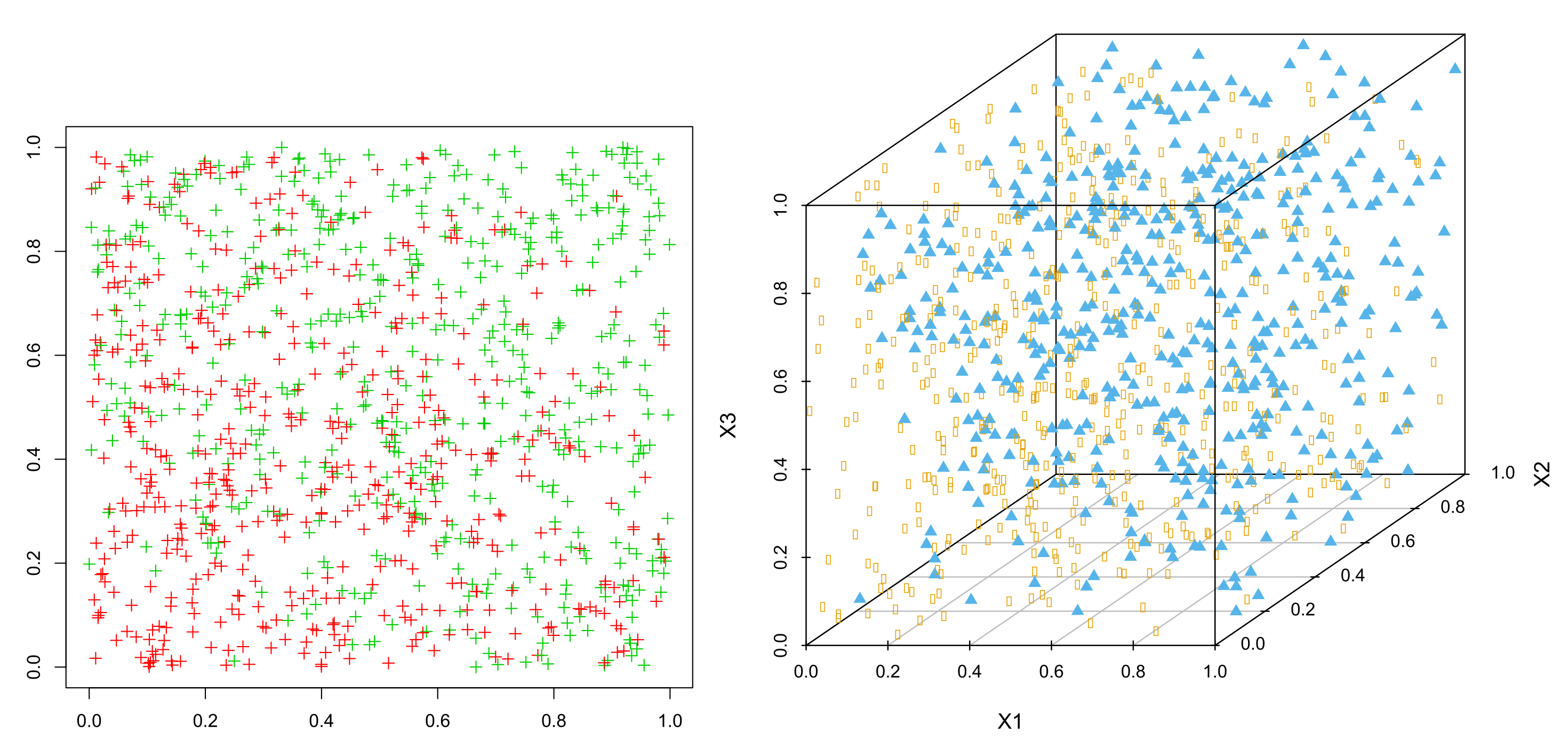
The second dataset corresponds to a simulation scheme for the problem of classifying two classes in a d-dimensional unit cube; the conditional probability of class $y=1$ given the d-dimensional vector x is

$$\eta \left(x\right)=P(y=1|x)=\frac{{\sum }_{i=1}^d{x}_i}{d}.$$

In Figure 2, the graphical representations in dimension 2 and dimension 3 are shown, labeling the classes with different colors.

For different dimension values d, we simulate 300,000 observations, using 240,000 observations as the training sample and 60,000 observations for testing. To determine parameter values, a cross-validation scheme is considered with an independent sample equal to 1% of the total, i.e., with 3000 observations. For this example, we only present the results for the case $d=20$.

The other datasets were taken from the LibSVM library (see [5] and https://www.csie.ntu.edu.tw/~cjlin/libsvm accessed on 1 May 2022).

4.3. Parameter Choices

For each problem and kernel, the choice of parameters is made before the local sampling SVM procedure, as described in the previous section, and it is run on the validation set (exclusive for this task) composed of 1% or 5% of the training data (5% in the smallest datasets) based on the results obtained on a small subsample of the training set. This subsample and the rest of the training set are disjointed from the test set. The parameters to be tuned in advance are the kernel parameters and the cost parameter C for the optimization problem as well as the parameter $\beta$ of our algorithm. The kernel parameters and C are chosen via 10-fold cross-validation of the optimization procedure on the small subsample. Once they are chosen, $\beta$ is selected by dividing the subsample into sets of 80% and 20%, using the larger of these sets to train our procedure for different values of $\beta$, starting from $\beta =0.1$ and incrementing it by 0.1 whenever a significant reduction of the classification error on the 20% part of the subsample is achieved.

With the parameters chosen, the SVM classifier was fitted on the full training sample using the libsvm solver: the number and class identity of support vectors were obtained, and the execution time for the full problem and the test error were obtained for the test set. In the summary tables, each kernel is indicated in the first column. In the second and third columns, we show the optimal parameters C and $\gamma$ obtained via cross-validation for each kernel function, the latter separated by row. The fourth column will show the number of support vectors for each kernel, followed by quantities in parentheses, which represent the division of support vectors by class. The accuracy rates obtained in the test set are presented in the fifth column. Finally, in the sixth column, the execution times are presented in seconds.

The local sampling approach was executed for the previously chosen value of $\beta$. As part of our analysis, we present the average results for 10 runs of the SVM solution considering our algorithm with the (fixed) optimal parameters C, $\gamma$, and $\beta$ obtained in the preliminary evaluation. We also report the initial amount of support vectors in step (ii) of the procedure, the number of support vectors at the end of the procedure, the number of these vectors that are SVs for the problem solved on the full training data set, the accuracy rate on the test data, and the execution times. In addition, we compare the results obtained using our proposed method and the procedure introduced in [4].

5. Numerical Results

5.1. Comparison with LibSVM and CGLQ

This subsection encompasses the results obtained for the problems tested using three kernels. For each of them, a description of how the local sampling algorithm is applied is included, and three tables are displayed. The first shows the results obtained when solving the problem using the full training set and implementing the libsvm methodology. Then, information on the classification error, the number of support vectors, and computational time are included.

Table 2. SVM results from libsvm 2D circle model data.

	Optimal Parameters
Kernel	Cost	$\mathbf{\gamma }$	Support Vectors	Accuracy	Time (s)
Linear	0.001	–	71,087 (35,544$\left|\right|$35,543)	0.554	172.38
Polynomial	10	5	40,398 (20,204$\left|\right|$20,194)	0.775	784.64
Radial basis	1	1	38,786 (19,407$\left|\right|$19,379)	0.774	518.17

,

Table 3. SVM results from libsvm 20D simulation.

	Optimal Parameters
Kernel	Cost	$\mathbf{\gamma }$	Support Vectors	Acc Rate	Time (s)
Linear	0.1	–	224,969 (112,482$\left|\right|$11,487)	0.551	8965
Polynomial	0.1	0.1	223,216 (111,608$\left|\right|$111,608)	0.548	9695.92
Radial basis	1	0.01	224,299 (112,134$\left|\right|$112,160)	0.551	16,820.63

,

Table 4. SVM results from libsvm COD-RNA training data.

	Optimal Parameters
Kernel	Cost	$\mathit{\gamma }$	Number of Support Vectors	Acc Rate	Time (s)
Linear	1	–	21,706 (10,856$\left|\right|$10,850)	0.7938	120.18
Polynomial	0.1	1	12,821 (6424$\left|\right|$6397)	0.7845	601.62
Radial basis	10	0.1	8768 (4380$\left|\right|$4388)	0.7574	121.9

,

Table 5. SVM results from LibSVM IJCNN1 training data.

	Optimal Parameters
Kernel	Cost	$\mathit{\gamma }$	Number of Support Vectors	Acc Rate	Time (s)
Linear	10	–	8146 (4077$\left|\right|$4089)	0.9219	50.34
Polynomial	5	0.1	8061 (4051$\left|\right|$4010)	0.9309	38.53
Radial basis	10	0.1	5497 (2763$\left|\right|$2734)	0.9722	69.95

,

Table 6. SVM results from LibSVM w7a data.

	Optimal Parameters
Kernel	Cost	$\mathit{\gamma }$	Number of Support Vectors	Acc Rate	Time (s)
Linear	1	–	696 (382$\left|\right|$314)	0.9893	181.01
Polynomial	0.1	1	802 (528$\left|\right|$279)	0.9823	58.61
Radial basis	10	0.01	5552 (4923$\left|\right|$629)	0.9843	365.57

,

Table 7. SVM results from LibSVM COVTYPE training data.

	Optimal Parameters
Kernel	Cost	$\mathit{\gamma }$	Number of Support Vectors	Acc Rate	Time (s)
Linear	10	–	299,256 (150,111$\left|\right|$149,145)	0.755	36,190.19
Polynomial	1	1	214,409 (107,190$\left|\right|$107,219)	0.833	39,504.57
Radial basis	10	5	143,154 (71,420$\left|\right|$71,734)	0.89	28,372.08

and

Table 8. SVM results from LibSVM WEBSPAM training data.

	Optimal Parameters
Kernel	Cost	$\mathit{\gamma }$	Number of Support Vectors	Acc Rate	Time (s)
Linear	10	–	56,213 (28,285$\left|\right|$27,928)	0.921	21,705.89
Polynomial	10	2	16,596 (8407$\left|\right|$8189)	0.973	16,205.77
Radial	10	2	16,389 (8644$\left|\right|$7745)	0.981	10,881.45

present the results.

The other tables ((

Table 9. Two-dimensional (2D) circle error and computing times vs. CGLQ algorithm.

(a) Local sampling SVM
2D Circle	Kernel
$\mathbf{\delta }=\mathbf{0}.\mathbf{1}$	Linear	Polynomial	Radial Basis
$\beta$	0.1	0.1	0.1
SV initial	7161	4095	4305
SV final	41,805	20,424	19,831
SV real	38,613	20,417	19,327
% full SV	54.31%	50.54%	49.83%
Accuracy	0.553	0.777	0.7252
Sd. dev.	(0)	(0.0004)	(0.003)
Acc ratio	−0.01	0.002	−0.063
Time (s)	52.98	86.67	94.239
% full time	30.73%	11.04%	18.18%
(b) CGLQ Algorithm
2D Circle	Kernel
$\mathbf{\delta }$= 0.1	Linear	Polynomial	Radial Basis
SV initial	7100	4038	3947
SV final	38,432	19,634	18,868
SV real	37,222	19,586	18,697
% full SV	52.36%	48.48%	48.207%
Acc rate	0.5538	0.732	0.776
Sd. dev.	(0)	(0.09)	(0.0005)
Acc ratio	−0.01	−0.056	0.001
Time (s)	51.01	122.69	104.36
% full time	29.59%	15.63%	20.14%

,

Table 10. 20D simulation error and computing times vs. CGLQ algorithm.

(a) Local sampling SVM
20D Unit Cube	Kernel
$\mathbf{\delta }\approx \mathbf{0}.\mathbf{01}$	Linear	Polynomial	Radial Basis
$\beta$	0.1	0.1	0.1
SV initial	2504	2992	2837
SV final	16,973	21,629	19,154
SV real	16,795	21,065	18,736
% full SV	7.46%	9.43%	8.35%
Acc rate	0.5521	0.5498	0.5519
Sd. dev.	(0.0006)	(0.00045)	(0.0006)
Acc ratio	0.001	0.003	0.001
Time (s)	155.907	225.13	253.703
% full time	1.73%	2.32%	1.5%
(b) CGLQ Algorithm
20D Unit Cube	Kernel
$\mathbf{\delta }\approx \mathbf{0}.\mathbf{01}$	Linear	Polynomial	Radial Basis
SV initial	2253	2342	2345
SV final	22,244	22,986	23,180
SV real	22,135	22,422	22,737
% full SV	9.83%	10.04%	10.13%
Acc rate	0.55	0.5279	0.5449
Sd. dev.	(0.002)	(0.002)	(0.0002)
Acc ratio	−0.002	−0.04	−0.02
Time (s)	5250.2	1875.5	10827.34
% full time	58.56%	19.34%	64.36%

,

Table 11. COD-RNA error and computing times vs. CGLQ algorithm.

(a) Local sampling SVM
COD-RNA	Kernel
$\mathbf{\delta }\approx 0.01$	Linear	Polynomial	Radial Basis
$\beta$	0.2	0.5	0.1
SV initial	282	320	356
SV final	1089	1566	581
SV real	982	1370	119
% full SV	4.52%	10.69%	1.36%
Acc rate	0.7863	0.7857	0.7524
Sd. dev.	(0.02)	(0.0014)	(0.012)
Acc ratio	−0.0009	0.001	−0.006
Time (s)	0.587	4.24	0.696
% full time	0.48%	0.7%	0.57%
(b) CGLQ Algorithm
COD-RNA	Kernel
$\mathbf{\delta }\approx 0.01$	Linear	Polynomial	Radial Basis
SV initial	232	155	188
SV final	1143	503	529
SV real	1057	401	111
% full SV	4.87%	3.12%	1.27%
Acc rate	0.7877	0.7698	0.7638
Sd. dev.	(0.0021)	(0.003)	(0.011)
Acc ratio	−0.007	−0.01	0.008
Time (s)	3.35	4.89	3.16
% full time	2.79%	0.72%	2.59%

,

Table 12. IJCNN1 error and computing times vs. CGLQ algorithm.

(a) Local sampling SVM
IJCNN1	Kernel
$\mathbf{\delta }\approx$0.02	Linear	Polynomial	Radial Basis
$\beta$	0.1	0.2	0.5
SV initial	329	461	403
SV final	633	423	1078
SV real	111	313	617
% full SV	1.36%	3.88%	11.22%
Acc rate	0.9254	0.9397	0.9706
Sd. dev.	(0.007)	(0.006)	(0.001)
Acc ratio	0.003	0.0094	−0.001
Time (s)	1.36	1.016	4.46
% time SVM	2.7%	2.63%	6.38%
(b) CGLQ Algorithm
IJCNN1	Kernel
$\mathbf{\delta }\approx$0.02	Linear	Polynomial	Radial Basis
SV initial	183	249	198
SV final	711	333	395
SV real	691	251	233
% full SV	8.48%	3.11%	3.75%
Acc rate	0.9293	0.9423	0.9679
Sd. dev.	(0.003)	(0.01)	(0.004)
Error ratio	0.008	0.012	−0.004
Time (s)	3.2	1.63	3.75
% time SVM	6.45%	4.24%	5.36%

,

Table 13. W7A error and computing times vs. CGLQ algorithm.

(a) Local sampling SVM
w7a	Kernel
$\mathbf{\delta }$= 0.1	Linear	Polynomial	Radial Basis
$\beta$	0.5	0.2	0.2
SV initial	490	1366	604
SV final	294	893	441
SV real	144	319	124
% full SV	20.76%	39.81%	2.24%
Acc rate	0.9829	0.9818	0.983
Sd. dev.	(0.001)	(0.001)	(0.008)
Acc ratio	−0.006	−0.0004	0.0009
Time (s)	7.75	14.51	8.99
% time SVM	4.28%	28.11%	2.46%
(b) CGLQ Algorithm
w7a	Kernel
$\mathbf{\delta }$= 0.1,$\mathit{K}$= 5	Linear	Polynomial	Radial Basis
SV initial	150	545	217
SV final	250	727	402
SV real	130	172	169
% full SV	18.64%	21.45%	3.05%
Acc rate	0.9819	0.9821	0.985
Sd. dev.	(0.002)	(0.0014)	(0.001)
Acc ratio	−0.007	−0.0002	0.0007
Time (s)	8.4	13.34	10.78
% time SVM	4.64%	25.84%	2.95%

,

Table 14. COVTYPE error and computing times vs. CGLQ algorithm.

(a) Local sampling SVM
COVTYPE	Kernel
$\mathbf{\delta }\approx$0.025	Linear	Polynomial	Radial Basis
$\beta$	0.1	0.2	0.1
SV initial	7774	6387	10,819
SV final	43,883	27,414	24,396
SV real	24,777	20,150	18,005
% full SV	8.17%	9.29%	12.48%
Acc rate	0.7614	0.8132	0.86
Sd. dev.	(0.0008)	(0.0004)	(0.001)
Acc ratio	−0.002	−0.024	−0.033
Time (s)	300.72	1228.55	789.406
% time SVM	0.82%	3.1%	2.74%
(b) CGLQ Algorithm
COVTYPE	Kernel
$\mathbf{\delta }\approx$0.025,$\mathit{K}$= 5	Linear	Polynomial	Radial Basis
SV initial	7474	5671	5627
SV final	40,039	26,248	19,146
SV real	23,189	19,044	5324
% full SV	7.74%	8.88%	3.71%
Acc rate	0.7630	0.829	0.876
Sd. dev.	(0.00002)	(0.0009)	(0.001)
Error ratio	0.0105	−0.004	−0.015
Time (s)	299.73	13,188.47	8887.25
% time SVM	0.82%	33.38%	15.79%

and

Table 15. WEBSPAM error and computing times vs. CGLQ algorithm.

(a) Local sampling SVM
WEBSPAM	Kernel
$\mathbf{\delta }$= 0.01	Linear	Polynomial	Radial Basis
$\beta$	0.1	0.5	0.2
SV initial	1490	1145	1344
SV final	5527	2187	2351
SV real	4897	2183	2351
% full SV	8.59%	13.01%	12.96%
Acc rate	0.923	0.9623	0.9727
Sd. dev.	(0.006)	(0.0026)	(0.0022)
Error ratio	0.002	−0.0109	−0.008
Time (s)	108.48	238.39	106.393
% time SVM	0.49%	1.44%	0.96%
(b) CGLQ Algorithm
WEBSPAM	Kernel
$\mathbf{\delta }$= 0.01	Linear	Polynomial	Radial Basis
SV initial	780	470	596
SV final	3214	1091	1602
SV real	3206	1090	1598
% full SV	5.704%	6.49%	9.61%
Acc rate	0.9239	0.959	0.9654
Sd. dev.	(0.0004)	(0.0004)	(0.0007)
acc ratio	0.0031	−0.013	−0.015
Time (s)	223.94	125.385	294.03
% time SVM	1.03%	0.77%	2.7%

), on each example, show the results obtained using the local sampling approach and the CGLQ algorithm from [4]. Each table contains the initial and final number of support vectors, and we also take the number and percentage they represent of the SVM methodology under the libsvm implementation, that is, the percentage of the support vectors found by the subsample procedures that are support vectors for the full dataset. We define the Accuracy ratio as

$$Ac{c}_{ratio}=\frac{Ac{c}_{L\mathcal{S}}}{Ac{c}_{\mathrm{libsvm}}}-1,$$

representing a measure of the proximity between the classification errors corresponding to the subsample procedures and the full dataset under libsvm. A positive value for this quotient indicates an improvement in the error when using the subsampling approach. The tables also include the execution time for the subsample procedures and the percentage that the computational time represents of the running time for the full dataset given by the libsvm routine.

5.2. Comparison with Other Methodologies

As an important part of our contribution, we present an interesting comparison regarding other approaches existing in the literature, such as the aforementioned LibSVM in [5], SVM${}^{light}$ [6], and a method based on decision trees from [27]. In the latter, the idea is to train SVM using significantly smaller refined training sets and label vectors from training as those closer or far from the decision hyperplane, after which a decision tree is used to find vectors with similar characteristics to those marked as support vectors. To conduct the contrasting, the metrics used before and two additional measures, which is appropriate to evaluate the performance of SVM, are considered. These are as follows:

• Proportion of Support Vectors ($PSV$) is a measure used to define the decision boundary:

  $$PSV=100·\frac{{\mathcal{N}}_{SV}}{n},$$

  where ${\mathcal{N}}_{SV}$ is the number of support vectors.
• Performance index for SVM, denoted as $P{I}_{SVM}$, has its antecedent in [39], where $PSV$ is combined with accuracy to guide the optimization of hyperparameters. In Rojas Dominguez et al. [40], this measure of SVM performance is defined as a function of accuracy and $PSV$. Provided that these are percentages, the performance index for SVM classifiers ($P{I}_{SVM}$) is given by:

  $$P{I}_{SVM}=exp\left(\frac{-k(PSV+{(100-Acc)}^2)}{200-PSV-Acc+ϵ}\right)$$

  where $k>0$ is a (small) constant factor that shapes the function and $ϵ$ is a small number to avoid division by zero.

The index $P{I}_{SVM}$ is bounded in $[0,1]$ and can be used as an alternative to the adequacy function based solely on accuracy appearing in most works found in the literature. Notice that contrary to the idea in [39], this does not describe a linear relationship between accuracy and $PSV$. Instead, it is employed to examine the performance of the algorithms, and in a final experiment, it is tested to lead to the optimization of the best algorithm identified.

We now compare our proposed method and three state-of-the-art methods: LibSVM, SVM${}^{light}$, and decision tree-based SVM. We implemented this exercise in R, selecting for each dataset the kernel function that had the best performance in the previous section in terms of precision and execution time for the libsvm fit with the full training sample.

Table 16. Comparison.

(a) libsvm performance
libsvmDataset	Measures
	Acc	Time	$\mathit{PSV}$	${\mathit{PI}}_{\mathit{SVM}}$
2D circle	77.5	784.64	50.49	0.4616
20D cube	55.1	8965	93.73	0.0162
COD RNA	79.38	120.18	38.37	0.5692
IJCNN1	97.22	69.95	11.57	0.979
W7A	98.93	181.01	2.95	0.9958
Covtype	89	28,372.08	27.75	0.8363
Webspam	98.1	10,081.45	5.51	0.9905
(b) ${\mathrm{SVM}}^{\mathit{light}}$ performance
${\mathrm{SVM}}^{\mathit{light}}$	Measures
	Acc	Time	$\mathit{PSV}$	${\mathit{PI}}_{\mathit{SVM}}$
2D circle	69.28	2818.97	55.16	0.2666
20D cube	55.19	1386.92	93.74	0.016
COD RNA	74.03	51.67	1.65	0.5805
IJCNN1	97.18	267.54	11.4763	0.9789
W7A	98.92	336.48	13.132	0.9829
Covtype	0.8846	39,546.7	33.674	0.8071
Webspam	97.36	23,774.4	18.53	0.9701
(c) Local sampling performance
Local Sampling	Measures
	Acc	Time	$\mathit{PSV}$	${\mathit{PI}}_{\mathit{SVM}}$
2D circle	77.7	86.67	25.53	0.5826
20D cube	55.21	155.9	7.07	0.2318
COD RNA	78.63	0.587	1.92	0.681
IJCNN1	97.06	4.46	2.26	0.9892
W7A	98.29	7.75	1.24	0.9959
Covtype	86.06	789.4	4.72	0.8332
Webspam	97.27	106.39	0.7915	0.9919
(d) Decision tree-based SVM performance
Dec. Tree SVM	Measures
	Acc	Time	$\mathit{PSV}$	${\mathit{PI}}_{\mathit{SVM}}$
2D circle	52.97	688.72	1.9	0.2175
20D cube	54.87	31.41	6.67	0.2286
COD RNA	79.74	1.56	3.47	0.701
IJCNN1	95.84	2.85	1.41	0.9819
W7A	98.15	2.64	0.8839	0.9957
Covtype	85.1	585.69	3.71	0.83162
Webspam	96.63	123.61	1.14	0.9878

is organized as follows. In the upper left corner, the results for the LibSVM implementation appear, which is followed by the SVM light method in the upper right. In the lower-left corner is our local sampling method, and finally, in the lower-right section is the output of the SVM decision tree-based methodology. The columns contain the set of observations, kernel function to be used, accuracy rate, execution time, proportion of support vectors, and performance index for SVM.

It can be seen in Table 16 that in terms of precision, the LibSVM approach outperforms the other methodologies in most cases, but for the simulated datasets (2D circle and 20D cube), the best precision performance is for the local sampling method, and only in the COD-RNA set the highest accuracy rate was obtained with the decision tree-based SVM.

5.3. Discussion

To summarize our analysis against the CGLQ methodology, we observe that both methods are very effective in terms of error rates in the simulated examples, but in many cases, local sampling achieves dramatic savings in computation time compared with CGLQ. On the real data examples, the results can be grouped as follows: In three of the datasets (COD-RNA, W7A, and COVTYPE), the performance in terms of the classification error is very similar, but local sampling offers savings in computational time, which is often important compared with CGLQ. Finally, on the WEBSPAM data, the results are very similar for both subsampling methods in terms of error rates, and which one is faster depends on the kernel considered.

Overall, we can say that the novel local sampling procedure outperforms the CGLQ methodology in most datasets. It appears that the local sampling implemented through bagging and importance sampling and the extra flexibility introduced by the parameter $\beta$, which controls the enriching subsampling regions’ size, pays off, resulting in a procedure that enriches the original samples more effectively.

Regarding the execution times, in the comparison in Section 4.2, we note that the best performance is provided by the decision tree approach as its formulation works efficiently: selecting only a subsample, working from it with the decision tree, and solving a problem of a much smaller size. This deteriorates its performance, and in that sense, we can say that our methodology is competitive, because the runtimes are smaller than those of the usual methodologies, and at least in three datasets (2D circle, COD RNA, and Webspam), the shortest execution times were reached.

Given the results of the last two columns of Table 16, we can say that our advantage is reflected in the two performance measures introduced: $PSV$ and $P{I}_{SVM}$. From the viewpoint of structural risk minimization, the term of the complexity of the model is given by the Vapnik–Chervonenkis (VC) dimension. In the case of SVM, it is provided by the VC dimension of the separating hyperplanes and is precisely related to the number of support vectors and the number of observations to be separated. With this reasoning, these indices naturally arise.

6. Conclusions

In the present work, theoretical results were presented that help understand the performance of subsampling methods in determining an approximate solution for the SVM problem for big data classification. We proved that under some conditions, there exists, with high probability, a feasible solution of the dual SVM problem for a randomly chosen training subsample, with the corresponding classifier as close as desired (in terms of classification error) to the classifier obtained from training with the complete dataset.

In addition, we introduced a local sampling methodology for SVM classification; this methodology is local because it uses information close to the observations of interest (support vectors). The bagging and local subsampling SVM methodology presented herein attains, in many problems, classification accuracy comparable to that corresponding to the solution of the problem on the full training sample, using a fraction of the training dataset and a smaller number of support vectors, thus producing significant savings on computational time.

Among the aspects to remark on, we highlight the analysis of the $P{I}_{SVM}$ measure as a general way of quantifying the training performance of support vector machine algorithms. It defines a tradeoff between accuracy and the number of support vectors used to achieve a given performance. Notice that in our context, it makes sense since we are searching for an optimal subsampling by trying to find the most support vectors. However, with a small proportion of the original support vectors ($PSV$) or observations close to these, it is possible to find a solution close enough to the SVM performance with the full dataset. In the practical implementation, we have that our $P{I}_{SVM}$ is the best for almost all datasets: 2D-Circle (0.58), 20D-Cube (0.2318), IJCNN1 (0.9882), W7A (0.9959) and WEBSPAM (0.9919).

In general, the proposed method compares favorably to the subsampling and nearest neighbors enriching methodology proposed in [4]. The advantages of the proposed methodology depend, to some extend, on the complexity of the problem and the kernel used in the algorithm; however, they are more noticeable when the dimension of the dataset is not very large. In the final comparison, the execution times are lower with respect to the total training time for routines such as LibSVM, where in our case, the highest percentage of time used of the total libsvm was 10.9% for the 2D-Circle set, whereas the rest are significantly lower, and the lowest was 0.48% in CODRNA. Here, we note that the best competitor in execution times is the algorithm of Cervantes et al. [27].

As limitations, we may mention the following: some experimental results have lower accuracy compared to other methodologies. This is due to the randomness of the subsampling method, although in most cases, the differences in performance are not significant. In those problems with higher dimensions, a so-called curse of dimensionality effect appears, deteriorating the accuracy. As the dimension increases, the effectiveness of the subsampling decreases, as shown in Equation (5).

At last, although there is flexibility in the choice of the beta parameter defining the subsampling rate, for some problems, it was not possible to find the best choice. Even extending the execution time, the algorithm did not gain in accuracy. Further research will consider this issue.

Finally, future work should address the following issues:

• Determine a theoretical result for quantifying the subsampling rate in terms of efficiency measures and the closeness to the final classification accuracy as well as the number of observations expected to be SV in an optimal search.
• An open issue is to explore the general key aspects of subsampling approaches and their potential contribution to training SVM methods involving hybrid-type algorithms.
• Consider unbalanced classification problems and their effect on local subsampling. Devote further effort to areas where we can locate observations from both classes. Otherwise, SVM will not be informative.
• Extend the discussion to multi-class problems and determine how subsampling schemes can work in such cases.