Bifurcation and Patterns Analysis for a Spatiotemporal Discrete Gierer-Meinhardt System

Abstract

The Gierer-Meinhardt system is one of the prototypical pattern formation models. The bifurcation and pattern dynamics of a spatiotemporal discrete Gierer-Meinhardt system are investigated via the couple map lattice model (CML) method in this paper. The linear stability of the fixed points to such spatiotemporal discrete system is analyzed by stability theory. By using the bifurcation theory, the center manifold theory and the Turing instability theory, the Turing instability conditions in flip bifurcation and Neimark–Sacker bifurcation are considered, respectively. To illustrate the above theoretical results, numerical simulations are carried out, such as bifurcation diagram, maximum Lyapunov exponents, phase orbits, and pattern formations.

1. Introduction

In Turing’s pioneering work, the diffusion terms on pattern formation for reaction diffusion systems are the main factor [1]. In recent decades, Turing instability has been investigated in biology, physics, chemistry, embryogenesis, and others [2,3,4,5].

Many biological, chemical and physical phenomena in nature can be described by the reaction diffusion equation, such as patterns and wave speeds. To describe the spatial patterns formation for the tissue structures in embryology and regeneration, Gierer and Meinhardt proposed several reaction diffusion equations–molecular models in 1972 [6]. The Gierer-Meinhardt system is expressed as the following form

$$\begin{array}{c}\hfill \left\{\begin{array}{c}\frac{\partial a(t,x,y)}{\partial t}={\rho }_0\rho +c\rho \frac{a^r(t,x,y)}{h^s}-\mu a(t,x,y)+d_1\Delta a(t,x,y),\hfill \\ \frac{\partial h(t,x,y)}{\partial t}=c^{\prime }{\rho }^{\prime }\frac{a^T(t,x,y)}{h^u}-vh(t,x,y)+d_2\Delta h(t,x,y),\hfill \end{array}\right.\end{array}$$

(1)

where $a(t,x,y)$ and $h(t,x,y)$ are the density of the activator and inhibitor at time $t>0$ and spatial location $(x,y)$ respectively. $d_1$ and $d_2$ are the constant diffusion parameters to the activator and inhibitor, respectively; $\rho {\rho }_0$ is the source concentration for the activator, here $\rho$ and ${\rho }^{\prime }$ are constants; ${\rho }^{\prime }$ is the one for the inhibitor; the activator and the inhibitor are removed by the first order kinetics $\mu a$ and $vh$, respectively.

Lots of works on the stability and bifurcation problems of stationary solutions and simulation research have been performed to study the dynamical behaviors of these systems [7,8,9,10,11,12,13,14,15], references therein. Ward and Wei [7] studied the stability and oscillatory instability of symmetric k-spike equilibrium solutions to the Gierer-Meinhardt reaction-diffusion system in a one-dimensional spatial domain for various ranges of the reaction-time constant and the diffusivity of the inhibitor field dynamics. Wei and Winter [8] constructed solutions with a single interior condensation point for the two-dimensional Gierer-Meinhardt system with strong coupling. Ruan [9] investigated the instability of equilibrium points and the periodic solutions under diffusive effects, which were stable without diffusion via the perturbation method for such model with common sources. When $r=2,s=2,T=1$ and $u=0$, Wang et al. [10] studied Hopf bifurcation and Turing instability to such a system. Turing instability to the semi-discrete Gierer-Meinhardt model was considered in [11], and Turing bifurcation and chaos for the spatiotemporal discrete Gierer-Meinhardt were studied in [12]. Wu et al. [15] studied Turing instability and Hopf bifurcation to such a system, when $r=2,s=1,T=2$ and $u=0$. The influence of gene expression time delay on the patterns to Gierer-Meinhardt system was explored [16], and the influence of fractional Laplacian on the multi-bump solutions to Gierer-Meinhardt system was explored [17]. Moreover, some properties of the development of retinotectal projections in amphibians and fish can be described by using the Gierer-Meinhardt system [18]. Most applications of Gierer-Meinhardt system can be seen in Refs. [19,20,21].

Noticed that the coupled map lattices (CMLs) method can illustrate the complex dynamics of competitive system [2], physics system [22], population model [18], etc. Due to the efficiency of its numerical experiments, it is becoming an important branch of nonlinear dynamics. Some existing methods and theoretical results can be applied to study the dynamics of the CMLs model [23,24,25,26,27,28]. In addition, the Neimark–Sacker bifurcation and Turing bifurcation analysis were investigated to spatiotemporal discrete nutrient-phytoplankton model with time delay in Ref. [29] by using such methods. We will investigate the model theoretically to determine the conditions for such bifurcations to a modified Gierer-Meinhardt system based on CMLs. Then, the influence of parameters on the patterns formation can be illustrated quantitatively. Hence, the CMLs model can give a better description and prediction of pattern formation, which has been applied to the phytoplankton–zooplankton model [27,28] and predator–prey model [30] for pattern formation.

In order to obtain the spatiotemporal discrete Gierer-Meinhardt system, the CMLs method apply to a modified Gierer-Meinhardt model in this paper. By stability and bifurcation analysis, there are many interesting dynamical behaviors which cannot be generalized by the corresponding continuous Gierer-Meinhardt system for the classical bifurcation analysis, such as defect patterns. In this paper, we find other mechanisms (for example, flip-Turing bifurcation, Neimark–Sacker–Turing bifurcation), except Turing instability mechanism. Based on the analysis of these mechanisms, the circle, spiral of spatial patterns are found.

The remainder of this paper is organized as follows. The Gierer-Meinhardt system with CMLs model and its stability analysis are developed in Section 2. The detailed theoretical analysis of flip, Neimark–Sacker, Turing bifurcation and co-dimensional 2 bifurcation (such as Neimark–Sacker–Turing bifurcation) are carried out for the spatiotemporal discrete Gierer-Meinhardt system in Section 3. Numerical simulations are provided to illustrate the theoretical results in Section 3 and show the dynamical behaviors and spatial patterns in Section 4.

2. Stability Analysis

In [15], the authors studied the continuous modified Gierer-Meinhardt system which has the following form

$$\begin{array}{c}\hfill \left\{\begin{array}{c}\frac{\partial a(t,x,y)}{\partial t}=c+\frac{a^2(t,x,y)}{h}-\mu a(t,x,y)+d_1\Delta a(t,x,y),\hfill \\ \frac{\partial h(t,x,y)}{\partial t}=a^2(t,x,y)-h(t,x,y)+d_2\Delta h(t,x,y),\hfill \end{array}\right.\end{array}$$

(2)

where $\Delta ={\partial }^2/\partial x^2+{\partial }^2/\partial y^2$ in this paper. $(x,y)$ is the spatial vector in two-dimensional space, which shows the position of $a(t,x,y)$ or $h(t,x,y)$. By discretizing the model (1), the CMLs model is developed as follows. One considers $n\times n$ lattices in a two-dimensional square domain. Each lattice is a site $(i,j),i,j=1,2,...,n$ includes two numbers which are the density of activator $a(i,j,t)$ and the density of inhibitor $h(i,j,t)$ at time $t=T_t+T_0$, where $T_0$ is initial time. Due to interactions and migration between two species, the density of two will vary with time. When discrete step increases from t to $t+1$, the CMLs dynamics of the activator and inhibitor consists of two stages; one is the “reaction" stage and the other is “dispersal” stage. The dispersal stage can be obtained by the spatiotemporal discrete of (1)

$$\begin{array}{c}\hfill \left\{\begin{array}{c}{a}_{(i,j,t)}^{{}^{\prime }}=a_{(i,j,t)}+\frac{\tau }{{\delta }^2}{d}_1{\Delta }_d{a}_{(i,j,t)},\hfill \\ h_{(i,j,t)}^{{}^{\prime }}=h_{(i,j,t)}+\frac{\tau }{{\delta }^2}{d}_1{\Delta }_d{h}_{(i,j,t)},\hfill \end{array}\right.\end{array}$$

(3)

where $\delta$ and $\tau$ are the space interval and time interval for discretizing Equation (1), respectively. The discrete forms of the Laplacian operator ${\Delta }_d$ which can be shown in the following

$$\begin{array}{c}\hfill \begin{array}{c}{\Delta }_d{a}_{(i,j,t)}=a_{(i+1,j,t)}+a_{(i-1,j,t)}+a_{(i,j+1,t)}+a_{(i,j-1,t)}-4a_{(i,j,t)},\hfill \\ {\Delta }_d{h}_{(i,j,t)}=h_{(i+1,j,t)}+h_{(i-1,j,t)}+h_{(i,j+1,t)}+h_{(i,j-1,t)}-4h_{(i,j,t)}.\hfill \end{array}\end{array}$$

(4)

According to [31], the reaction terms can be obtained by discretizing the time terms of Equation (3)

$$\begin{array}{c}\hfill \begin{array}{c}{a}_{(i,j,t)}=f_1(a_{(i,j,t)},h_{(i,j,t)}),\hfill \\ h_{(i,j,t)}=g_1(a_{(i,j,t)},h_{(i,j,t)}),\hfill \end{array}\end{array}$$

(5)

where

$$\begin{array}{c}\hfill \begin{array}{c}{f}_1(a,h)=a+\tau (c+\frac{a^2}{h}-\mu a),\hfill \\ g_1(a,h)=h+\tau (a^2-h).\hfill \end{array}\end{array}$$

(6)

Assume that all the parameters are non-negative and $a_{(i,j,t)}$ and $h_{(i,j,t)}$ are non-negative. The periodic boundary conditions to the CMLs models are considered in this paper.

$$\begin{array}{c}\hfill \begin{array}{c}{a}_{(i,0,t)}=a_{(i,n,t)},a_{(i,1,t)}=a_{(i,n+1,t)},a_{(0,j,t)}=a_{(n,j,t)},a_{(1,j,t)}=a_{(n+1,j,t)},\hfill \\ h_{(i,0,t)}=h_{(i,n,t)},h_{(i,1,t)}=h_{(i,n+1,t)},h_{(0,j,t)}=h_{(n,j,t)},h_{(1,j,t)}=h_{(n+1,j,t)}.\hfill \end{array}\end{array}$$

(7)

For all $i,j,t$ satisfy

$$\begin{array}{c}\hfill {\Delta }_d{a}_{(i,j,t)}=0,{\Delta }_d{h}_{(i,j,t)}=0.\end{array}$$

Based on the above analysis, the homogeneous dynamics can be determined by

$$\begin{array}{c}\hfill \begin{array}{c}{a}_{t+1}=a_t+\tau (c+\frac{a_t^2}{h_t}-\mu a_t),\hfill \\ h_{t+1}=h_t+\tau (a_t^2-h_t).\hfill \end{array}\end{array}$$

(8)

Then, the Equation (8) can be rewritten into the form of maps equation

$$\begin{array}{c}\hfill \left(\begin{array}{c}a\\ h\end{array}\right)\mapsto \left(\begin{array}{c}a+\tau (c+\frac{a^2}{h}-\mu a)\\ h+\tau (a^2-h)\end{array}\right).\end{array}$$

(9)

Hence, the homogeneous dynamics of equations can be directly analyzed by maps Equation (9).

The fixed points of maps Equation (9) are the solutions of the following system

$$\begin{array}{c}\hfill \left\{\begin{array}{c}a=a+\tau (c+\frac{a^2}{h}-\mu a),\hfill \\ h=h+\tau (a^2-h).\hfill \end{array}\right.\end{array}$$

(10)

Clearly, system (10) has a unique fixed point $(a_{\ast },h_{\ast })=(\frac{c+1}{\mu },\frac{{(c+1)}^2}{{\mu }^2})(0<c<1)$. The Jacobian matrix associated to point $(a_{\ast },h_{\ast })$ is defined by

$$\begin{array}{c}\hfill {\left.J\right|}_{(a_{\ast },h_{\ast })}=\left(\begin{array}{c}\begin{array}{cc}1+\tau \mu \frac{1-c}{1+c}\hfill & -\frac{\tau {\mu }^2}{{(1+c)}^2}\end{array}\\ \begin{array}{cc}\hfill \frac{2(1+c)}{\mu }\tau & 1-\tau \end{array}\end{array}\right).\end{array}$$

(11)

According to [32], the fixed point is stable, if the two eigenvalues of ${\left.J\right|}_{(a_{\ast },h_{\ast })}$ satisfy $|{\lambda }_1|<1$ and $|{\lambda }_2|<1$. However, if the two eigenvalues satisfy $|{\lambda }_1|>1$ or $|{\lambda }_2|>1$, the fixed point is unstable. The two eigenvalues of ${\left.J\right|}_{(a_{\ast },h_{\ast })}$ are ${\lambda }_{1,2}=\frac{1}{2}\left(-p\left(\tau \right)\pm \sqrt{p^2\left(\tau \right)-4q\left(\tau \right)}\right)$, where $p\left(\tau \right)=\tau (1-\frac{1-c}{1+c}\mu )-2$ and $q\left(\tau \right)=\mu {\tau }^2+(\frac{1-c}{1+c}\mu -1)\tau +1$. If $q\left(\tau \right)<1$ and $\left|p\right(\tau \left)\right|<1+q\left(\tau \right)$, the fixed point $(a_{\ast },h_{\ast })$ is stable. By solving the above inequalities, we have the following result.

Proposition 1.

The fixed point $(a_{\ast },h_{\ast })$ is stable, if one of the following conditions is satisfied.

$$\begin{array}{c}\hfill \begin{array}{c}\left(H1\right):\left\{\begin{array}{c}0<\mu \le 3-2\sqrt{2},\hfill \\ 0<\tau <{\tau }_f.\hfill \end{array}\right.\left(H2\right):\left\{\begin{array}{c}3-2\sqrt{2}<\mu <\frac{1}{4},\hfill \\ \frac{4\mu \sqrt{\mu }+4\mu +{\mu }^2-1}{{(\mu -1)}^2}<c<1,\hfill \\ 0<\tau <{\tau }_f.\hfill \end{array}\right.\hfill \\ \left(H3\right):\left\{\begin{array}{c}3-2\sqrt{2}<\mu <\frac{1}{4},\hfill \\ 0<c\le \frac{4\mu \sqrt{\mu }+4\mu +{\mu }^2-1}{{(\mu -1)}^2},\hfill \\ 0<\tau <{\tau }_N.\hfill \end{array}\right.\left(H4\right):\left\{\begin{array}{c}\frac{1}{4}\le \mu \le 1,\hfill \\ 0<\tau <{\tau }_N.\hfill \end{array}\right.\left(H5\right):\left\{\begin{array}{c}\mu >1,\hfill \\ \frac{\mu -1}{1+\mu }<c<1,\hfill \\ 0<\tau <{\tau }_N.\hfill \end{array}\right.\hfill \end{array}\end{array}$$

(12)

In addition, if $\left(H1\right)$ or $\left(H2\right)$ holds, the fixed point $(a_{\ast },h_{\ast })$ is a stable node. If one of the conditions $\left(H3\right)$–$\left(H5\right)$ holds, it is a stable focus. Here, ${\tau }_N=\frac{1+c-\mu +c\mu }{(1+c)\mu }$ and ${\tau }_f={\tau }_N-\sqrt{{\tau }_N^2-4/\mu }$.

3. Bifurcation Analysis

In this section, taking $\tau$ as the critical bifurcation parameter, we will investigate flip, Naimark–Sacker, Turing bifurcation of system (3).

3.1. Flip Bifurcation

As known, if the fixed point $(a_{\ast },h_{\ast })$ loses its stability and undergoes a flip bifurcation, then the period-2 points are bifurcated from the fixed point. At the critical value of flip bifurcation, the two eigenvalues of J are ${\lambda }_1\left(\tau \right)=-1$ and $|{\lambda }_2\left(\tau \right)|\ne 1$. Hence, the bifurcation $\tau$ satisfies the following conditions:

$$\begin{array}{c}\hfill \tau ={\tau }_f,{\tau }_f(1-\frac{1-c}{1+c}\mu )\ne 2,4.\end{array}$$

(13)

The center manifold reduction can be applied to determine the stability of the bifurcated periodic-2 points. Taking $\tau$ as an independent, the center manifold reduction should be applied variable into the maps (9), and let $w=a-a_{\ast },z=h-h_{\ast }$ and $\overline{\tau }=\tau -{\tau }_f$; hence, the maps (9) is turned into the following form

$$\begin{array}{c}\hfill \left(\begin{array}{c}w\\ z\\ \overline{\tau }\end{array}\right)\mapsto \left(\begin{array}{ccc}{a}_{100}& a_{010}& 0\\ b_{100}& b_{010}& 0\\ 0& 0& 1\end{array}\right)\left(\begin{array}{c}w\\ z\\ \overline{\tau }\end{array}\right)+\left(\begin{array}{c}{f}_1(w,z,\overline{\tau })\\ g_1(w,z,\overline{\tau })\\ 0\end{array}\right)\end{array}$$

(14)

where

$$\begin{array}{cc}\hfill f_1(w,z,\overline{\tau })& =a_{200}{w}^2+a_{110}wz+a_{101}w\overline{\tau }+a_{011}z\overline{\tau }+a_{300}{w}^3+a_{210}{w}^{2}z+a_{201}{w}^2\overline{\tau }+a_{111}wz\overline{\tau }+\mathcal{O}\left(4\right),\hfill \\ \hfill g_1(w,z,\overline{\tau })& =b_{200}{w}^2+b_{110}wz+b_{101}w\overline{\tau }+b_{011}z\overline{\tau }+b_{300}{w}^3+b_{210}{w}^{2}z+b_{201}{w}^2\overline{\tau }+b_{111}wz\overline{\tau }+\mathcal{O}\left(4\right).\hfill \end{array}$$

Moreover, $\mathcal{O}\left(4\right)$ represents high order (≥4) in the variables $(w,z,\tau )$, and

$$\begin{array}{cc}\hfill a_{200}& =2\tau \frac{{\mu }^2}{{(c+1)}^2},a_{110}=-2\tau \frac{{\mu }^3}{{(c+1)}^3},a_{101}=\frac{\mu (1-c)}{c+1},a_{011}=\frac{-{\mu }^2}{{(c+1)}^2},\hfill \\ \hfill a_{300}& =0,a_{210}=\frac{-\tau {\mu }^2}{{(c+1)}^2},a_{201}=\frac{2{\mu }^2}{{(c+1)}^2},a_{111}=\frac{-2\mu }{c+1},b_{200}=2\tau ,\hfill \\ \hfill b_{110}& =\frac{2\tau \mu }{c+1},b_{011}=-1,b_{101}=\frac{2\mu }{c+1},b_{201}=2,b_{210}=b_{300}=b_{111}=0.\hfill \end{array}$$

Let

$$\begin{array}{c}\hfill \left(\begin{array}{c}w\\ z\\ \overline{\tau }\end{array}\right)=\left(\begin{array}{ccc}{a}_{100}& a_{010}& 0\\ -1-a_{100}& {\lambda }_2-a_{100}& 0\\ 0& 0& 1\end{array}\right)\left(\begin{array}{c}\tilde{a}\\ \tilde{h}\\ \tilde{\tau }\end{array}\right),\end{array}$$

(15)

where ${\lambda }_2=1-p\left({\tau }_f\right)$, and the maps (15) can be transformed into

$$\begin{array}{c}\hfill \left(\begin{array}{c}\tilde{a}\\ \tilde{h}\\ \tilde{\tau }\end{array}\right)=\left(\begin{array}{ccc}-1& 0& 0\\ 0& {\lambda }_2& 0\\ 0& 0& 1\end{array}\right)\left(\begin{array}{c}\tilde{a}\\ \tilde{h}\\ \tilde{\tau }\end{array}\right)+\frac{1}{a_{010}(1+{\lambda }_2)}\left(\begin{array}{c}{F}_1(\tilde{a},\tilde{h},\tilde{\tau })\\ F_2(\tilde{a},\tilde{h},\tilde{\tau })\\ 0\end{array}\right),\end{array}$$

(16)

where

$$\begin{array}{c}\begin{array}{cc}{F}_1(\tilde{a},\tilde{h},\tilde{\tau })=\hfill & a_{010}[({\lambda }_2-a_{100})a_{101}-a_{010}{b}_{101}](\tilde{a}+\tilde{h})\tilde{\tau }+a_{010}^2[({\lambda }_2-a_{100})a_{200}-a_{010}{b}_{200}]{(\tilde{a}+\tilde{h})}^2\hfill \\ \hfill & +a_{010}^2[({\lambda }_2-a_{100})a_{201}-a_{010}{b}_{201}]{(\tilde{a}+\tilde{h})}^2\tilde{\tau }+a_{010}^3[({\lambda }_2-a_{100})a_{300}-a_{010}{b}_{300}]{(\tilde{a}+\tilde{h})}^2\hfill \\ \hfill & +a_{010}[({\lambda }_2-a_{100})a_{110}-a_{010}{b}_{110}][\tilde{a}(-1-a_{100})+\tilde{h}({\lambda }_2-a_{100})](\tilde{a}+\tilde{h})\tilde{\tau }\hfill \\ \hfill & +a_{010}^2[({\lambda }_2-a_{100})a_{111}-a_{010}{b}_{111}][\tilde{a}(-1-a_{100})+\tilde{h}({\lambda }_2-a_{100})](\tilde{a}+\tilde{h})\tilde{\tau }\hfill \\ \hfill & +a_{010}^2[({\lambda }_2-a_{100})a_{210}-a_{010}{b}_{210}][\tilde{a}(-1-a_{100})+\tilde{h}({\lambda }_2-a_{100})]{(\tilde{a}+\tilde{h})}^2\hfill \\ \hfill & +[({\lambda }_2-a_{100}{a}_{011}][\tilde{a}(-1-a_{100})+\tilde{h}({\lambda }_2-a_{100})]\tilde{\tau },\hfill \\ F_2(\tilde{a},\tilde{h},\tilde{\tau })=\hfill & a_{010}[(1+a_{100})a_{101}+a_{010}{b}_{101}](\tilde{a}+\tilde{h})\tilde{\tau }+a_{010}^2[(1+a_{100})a_{200}+a_{010}{b}_{200}]{(\tilde{a}+\tilde{h})}^2\hfill \\ \hfill & +a_{010}^2[(1+a_{100})a_{201}+a_{010}{b}_{201}]{(\tilde{a}+\tilde{h})}^2\tilde{\tau }+a_{010}^3[(1+a_{100})a_{300}+a_{010}{b}_{300}]{(\tilde{a}+\tilde{h})}^2\hfill \\ \hfill & +a_{010}[(1+a_{100})a_{110}+a_{010}{b}_{110}][\tilde{a}(-1-a_{100})+\tilde{h}({\lambda }_2-a_{100})](\tilde{a}+\tilde{h})\tilde{\tau }\hfill \\ \hfill & +a_{010}^2[(1+a_{100})a_{111}+a_{010}{b}_{111}][\tilde{a}(-1-a_{100})+\tilde{h}({\lambda }_2-a_{100})](\tilde{a}+\tilde{h})\tilde{\tau }\hfill \\ \hfill & +a_{010}^2[(1+a_{100})a_{210}+a_{010}{b}_{210}][\tilde{a}(-1-a_{100})+\tilde{h}({\lambda }_2-a_{100})]{(\tilde{a}+\tilde{h})}^2\hfill \\ \hfill & +\left[(1+a_{100})a_{011}\right][\tilde{a}(-1-a_{100})+\tilde{h}({\lambda }_2-a_{100})]\tilde{\tau }.\hfill \end{array}\end{array}$$

The center manifold

$$W^c(0,0,0)=\{(\tilde{a},\tilde{h},\tilde{\tau })\in R^3|\tilde{h}=H(\tilde{a},\tilde{\tau }),H(0,0)=0,DH(0,0)=0\},$$

where $H(\tilde{a},\tilde{\tau })=e_1{\tilde{p}}^2+e_2\tilde{p}\tilde{\tau }+e_3{\tilde{\tau }}^2+\mathcal{O}\left(3\right)$. Using the invariance of the center manifold, taking $\tilde{h}=H(\tilde{a},\tilde{\tau })$ into the maps, and completing the coefficients of $e_j,j=1,2,3$, then

$$\begin{array}{cc}\hfill e_1& =\frac{{(1+a_{100})}^2{a}_{110}-(1+a_{100})(a_{200}-b_{110})a_{010}-a_{010}^2{b}_{200}}{{\lambda }_2^2-1},\hfill \\ \hfill e_2& =\frac{{(1+a_{100})}^2{a}_{011}-a_{010}(1+a_{100})a_{101}+a_{010}{b}_{101}}{a_{010}({\lambda }_2^2+1)},\hfill \\ \hfill e_3& =0.\hfill \end{array}$$

The maps (16) reduced to the central manifold $W^c(0,0,0)$ are the following form.

$$\begin{array}{c}\hfill F:\tilde{a}\mapsto -\tilde{a}+c_{20}{\tilde{a}}^2+c_{11}\tilde{a}\tilde{\tau }+c_{21}{\tilde{a}}^2\tilde{\tau }+c_{12}\tilde{a}{\tilde{\tau }}^2+c_{30}{\tilde{a}}^3+\mathcal{O}\left(4\right),\end{array}$$

(17)

here,

$$\begin{array}{cc}\hfill c_{20}& =\frac{1}{1+{\lambda }_2}\{(1+a_{100})a_{010}{b}_{110}-a_{010}^2{b}_{200}-2(1+a_{100})a_{110}+2a_{010}{a}_{200}\},\hfill \\ \hfill c_{11}& =\frac{1}{a_{010}(1+{\lambda }_2)}\{2a_{010}{a}_{101}-2a_{011}(1+a_{100})-a_{010}^2{b}_{101}\},\hfill \\ \hfill c_{12}& =\frac{e_2}{a_{110}(1+{\lambda }_2)}(4a_{011}+2a_{010}{a}_{101}-a_{010}^2{b}_{101}),\hfill \\ \hfill c_{21}& =\frac{1}{a_{010}(1+{\lambda }_2)}\left(\begin{array}{c}2a_{010}(2a_{010}{a}_{200}-a_{010}{b}_{110}+2a_{110}-a_{010}^2{b}_{200})e_2\\ +a_{010}(1+a_{100})(a_{010}{b}_{111}-2a_{111})+a_{010}^2(2a_{201}-a_{010}{b}_{201})\\ +(4a_{011}+2a_{010}{a}_{101}-a_{010}^2{b}_{101})e_1+(1+a_{100})(a_{010}{b}_{110}-2a_{110})a_{010}{e}_2\end{array}\right),\hfill \\ \hfill c_{30}& =\frac{1}{1+{\lambda }_2}\left(\begin{array}{c}{a}_{010}(1+a_{010})(a_{010}{b}_{201}-2a_{201})+a_{001}^2(2a_{300}-a_{010}{b}_{300})\\ +2(2a_{101}+2a_{010}{a}_{200}-a_{010}^2{b}_{200})e_1+(1+a_{100})(a_{010}{b}_{110}-2a_{101})e_1\end{array}\right).\hfill \end{array}$$

The occurrence of flip bifurcation for maps (17) also requires the flip bifurcation theorem in [33].

$$\begin{array}{cc}\hfill {\eta }_1& ={\left.(\frac{{\partial }^{2}F}{\partial \tilde{a}\partial \tilde{\tau }}+\frac{1}{2}\frac{\partial F}{\partial \tilde{\tau }}\frac{{\partial }^{2}F}{\partial {\tilde{a}}^2})\right|}_{(\tilde{a},\tilde{h})=(0,0)}=c_{11}\ne 0,\hfill \end{array}$$

(18)

$$\begin{array}{cc}\hfill {\eta }_2& ={\left.(\frac{1}{6}\frac{{\partial }^{3}F}{\partial {\tilde{a}}^3}+{(\frac{1}{2}\frac{{\partial }^{2}F}{\partial {\tilde{a}}^2})}^2)\right|}_{(\tilde{a},\tilde{h})=(0,0)}=c_{30}+c_{20}^2\ne 0.\hfill \end{array}$$

(19)

Theorem 1.

Assume the ($H1$) or ($H2$) holds, and ${\tau }_f(1-\frac{1-c}{1+c}\mu )\ne 2,4,{\eta }_1\ne 0,{\eta }_2\ne 0$, then the maps (9) undergo a flip bifurcation at $(a_{\ast },h_{\ast })$. Moreover, if ${\eta }_2>0(<0)$ is satisfied, the stable (unstable) periodic-2 points bifurcate from $(a_{\ast },h_{\ast })$.

3.2. Neimark–Sacker Bifurcation

The Neimark–Sacker bifurcation occurs at the fixed point $(a_{\ast },h_{\ast })$ of maps (9); there exists a pair of conjugate complex eigenvalues of the maps (9); in addition, the modules of two eigenvalues are both 1, which means $p\left(\tau \right)-4q\left(\tau \right)<0$ and $q\left(\tau \right)=1$. Hence

$$\begin{array}{c}\hfill \tau ={\tau }_N,0<{\tau }^2<\frac{4}{\mu }.\end{array}$$

(20)

In addition, the Neimark–Sacker bifurcation theorem [32,33] requires the tranversality condition to be non-zero; in fact

$$\begin{array}{c}\hfill d=\frac{d\left|\lambda \right({\tau }_N\left)\right|}{d\tau }=1-\frac{1-c}{1+c}\mu >0.\end{array}$$

(21)

Moreover, $\lambda {\left({\tau }_N\right)}^m\ne 1,m=1,2,3,4,$ i.e., $p\left({\tau }_N\right)\ne -2,0,1,2$.

Let $w=a-a_{\ast }$ and $z=h-h_{\ast }$, the map (9) becomes

$$\begin{array}{c}\hfill \left(\begin{array}{c}w\\ z\end{array}\right)\mapsto \left(\begin{array}{cc}{a}_{10}& a_{01}\\ b_{10}& b_{01}\end{array}\right)\left(\begin{array}{c}w\\ z\end{array}\right)+\left(\begin{array}{c}{a}_{20}{w}^2+a_{11}wz+a_{21}{w}^{2}z+a_{30}{w}^3+\mathcal{O}\left(4\right)\\ b_{20}{w}^2+b_{11}wz+b_{21}{w}^{2}z+b_{30}{w}^3+\mathcal{O}\left(4\right)\end{array}\right),\end{array}$$

(22)

where

$$\begin{array}{cc}\hfill a_{10}& =\frac{\mu (1-c){\tau }_N}{c+1},a_{01}=\frac{-{\mu }^2{\tau }_N}{{(c+1)}^2},a_{20}=2{\tau }_N\frac{{\mu }^2}{{(c+1)}^2},a_{11}=-2{\tau }_N\frac{{\mu }^3}{{(c+1)}^3},a_{21}=\frac{-{\tau }_N{\mu }^2}{{(c+1)}^2},\hfill \\ \hfill a_{30}& =0,b_{01}=-{\tau }_N,b_{10}=\frac{2\mu {\tau }_N}{c+1},b_{20}=2{\tau }_N,b_{11}=\frac{2{\tau }_N\mu }{c+1},b_{21}=0,b_{30}=0.\hfill \end{array}$$

The corresponding two eigenvalues are

$$\begin{array}{c}\hfill {\lambda }_{\pm }\left({\tau }_N\right)=\frac{-p\left({\tau }_N\right)}{2}\pm \frac{I}{2}\sqrt{4q\left({\tau }_N\right)-p^2\left({\tau }_N\right)}:=\alpha \pm I\beta ,\end{array}$$

(23)

where $I^2=-1$.

Assume

$$\begin{array}{c}\hfill \left(\begin{array}{c}w\\ z\end{array}\right)=\left(\begin{array}{cc}{a}_{01}& 0\\ \alpha -a_{10}& -\beta \end{array}\right)\left(\begin{array}{c}\tilde{a}\\ \tilde{h}\end{array}\right),\end{array}$$

(24)

then

$$\begin{array}{c}\hfill \left(\begin{array}{c}\tilde{a}\\ \tilde{h}\end{array}\right)=\left(\begin{array}{cc}\alpha & -\beta \\ \beta & \alpha \end{array}\right)\left(\begin{array}{c}\tilde{a}\\ \tilde{h}\end{array}\right)+\frac{1}{a_{01}\beta }\left(\begin{array}{c}{G}_1(\tilde{a},\tilde{h})\\ G_1(\tilde{a},\tilde{h})\end{array}\right),\end{array}$$

(25)

here,

$$\begin{array}{cc}\hfill G_1(\tilde{a},\tilde{h})=& (a_{20}{a}_{01}-(\alpha -a_{10})a_{11})a_{01}\beta {\tilde{a}}^2-a_{11}{a}_{01}{\beta }^2\tilde{a}\tilde{h}\hfill \\ \hfill & +(a_{30}{a}_{01}-(\alpha -a_{10})a_{21})a_{01}^2\beta {\tilde{a}}^3-b{a}_{21}{a}_{01}^2\beta {\tilde{a}}^2\tilde{h}+\mathcal{O}\left(4\right),\hfill \\ \hfill G_1(\tilde{a},\tilde{h})=& [(a_{11}(\alpha -a_{10})+a_{01}(a_{20}-b_{11}))(\alpha -a_{10})-b_{20}{a}_{01}^2]a_{01}{\tilde{a}}^2\hfill \\ \hfill & +[(a_{21}(\alpha -a_{10})+a_{01}(a_{30}-b_{21}))(\alpha -a_{10})-b_{30}{a}_{01}^2]a_{01}^2{\tilde{a}}^3\hfill \\ \hfill & -a_{01}(a_{11}(\alpha -a_{10})-b_{11}{a}_{01})\beta \tilde{a}\tilde{h}-a_{01}^2(a_{21}(\alpha -a_{10})-b_{21}{a}_{01})\beta {\tilde{a}}^2\tilde{h}+\mathcal{O}\left(4\right).\hfill \end{array}$$

In addition, the Neimark–Sacker bifurcation [33] requires the discriminatory quantity $\sigma$ satisfy

$$\begin{array}{c}\hfill \sigma =-Re(\frac{(1-2\lambda ){\overline{\lambda }}^2}{1-\lambda }{\xi }_{11}{\xi }_{20})-\frac{1}{2}|{\xi }_{11}{|}^2-{\left|{\xi }_{02}\right|}^2+Re\left(\overline{\lambda {\xi }_{21}}\right)\ne 0,\end{array}$$

(26)

where

$$\begin{array}{cc}\hfill {\xi }_{20}& =\frac{1}{8a_{01}\beta }[(G_{1\tilde{a}\tilde{a}}-G_{1\tilde{h}\tilde{h}}+2G_{2\tilde{a}\tilde{h}})+I(G_{2\tilde{a}\tilde{a}}-G_{2\tilde{h}\tilde{h}}-2G_{1\tilde{a}\tilde{h}})],\hfill \\ \hfill {\xi }_{11}& =\frac{1}{4a_{01}\beta }[G_{1\tilde{a}\tilde{a}}+G_{1\tilde{h}\tilde{h}}+I(G_{2\tilde{a}\tilde{a}}+G_{2\tilde{h}\tilde{h}})],\hfill \\ \hfill {\xi }_{02}& =\frac{1}{8a_{01}\beta }[(G_{1\tilde{a}\tilde{a}}-G_{1\tilde{h}\tilde{h}}-2G_{2\tilde{a}\tilde{h}})+I(G_{2\tilde{a}\tilde{a}}+G_{2\tilde{h}\tilde{h}}-2G_{1\tilde{a}\tilde{h}})],\hfill \\ \hfill {\xi }_{21}& =\frac{1}{16a_{01}\beta }[G_{1\tilde{a}\tilde{a}\tilde{a}}+G_{1\tilde{a}\tilde{h}\tilde{h}}+G_{2\tilde{a}\tilde{a}\tilde{h}}+G_{2\tilde{h}\tilde{h}\tilde{h}}+I(G_{2\tilde{a}\tilde{a}\tilde{a}}+G_{2\tilde{a}\tilde{h}\tilde{h}}-G_{1\tilde{a}\tilde{a}\tilde{h}}-G_{1\tilde{h}\tilde{h}\tilde{h}})].\hfill \end{array}$$

with

$$\begin{array}{cc}\hfill G_{1\tilde{a}\tilde{a}}& =\beta (2(\alpha -a_{01})a_{01}{a}_{11}+2a_{01}^2{a}_{20}),G_{1\tilde{a}\tilde{h}}=-{\beta }^2{a}_{01}{a}_{11},G_{1\tilde{h}\tilde{h}}=0,G_{1\tilde{a}\tilde{h}\tilde{h}}=0,\hfill \\ \hfill G_{1\tilde{h}\tilde{h}\tilde{h}}& =0,G_{1\tilde{h}\tilde{h}\tilde{h}}=\beta (6(\alpha -a_{01})a_{01}^2{a}_{11}+6a_{01}^3{a}_{30}),G_{1\tilde{a}\tilde{a}\tilde{h}}=-2{\beta }^2{a}_{01}^2{a}_{11},\hfill \\ \hfill G_{2\tilde{a}\tilde{a}}& =2a_{01}({(\alpha -a_{01})}^2{a}_{11}-a_{01}((\alpha -a_{01})(b_{11}-a_{20})+a_{01}{b}_{20})),G_{2\tilde{h}\tilde{h}}=0,G_{2\tilde{a}\tilde{h}\tilde{h}}=0,\hfill \\ \hfill G_{2\tilde{h}\tilde{h}\tilde{h}}& =0,G_{2\tilde{a}\tilde{h}}=\beta a_{01}((a_{01}-\alpha )a_{11}+a_{01}{b}_{11}),G_{2\tilde{a}\tilde{a}\tilde{h}}=2\beta a_{01}^2((a_{01}-\alpha )a_{11}+a_{01}{b}_{11}),\hfill \\ \hfill G_{2\tilde{h}\tilde{h}\tilde{h}}& =6a_{01}^2((\alpha -a_{01})a_{21}-a_{01}((\alpha -a_{01})(b_{21}-a_{30})+a_{01}{b}_{30})),\hfill \end{array}$$

which are the second and third order partial derivatives of $G_1(a_{\ast },h_{\ast })$ and $G_2(a_{\ast },h_{\ast })$ at $(0,0)$.

Theorem 2.

Assume one of the conditions ($H3$)–($H5$) holds. If $\sigma \ne 0$, then map (9) undergoes Neimark–Sacker bifurcation at the fixed point $(a_{\ast },h_{\ast })$ when $\tau ={\tau }_N$. In addition, if $\sigma <0(>0)$, then an attracting (a repelling) invariant circle will occur when $\tau >{\tau }_N(0<\tau <{\tau }_N)$.

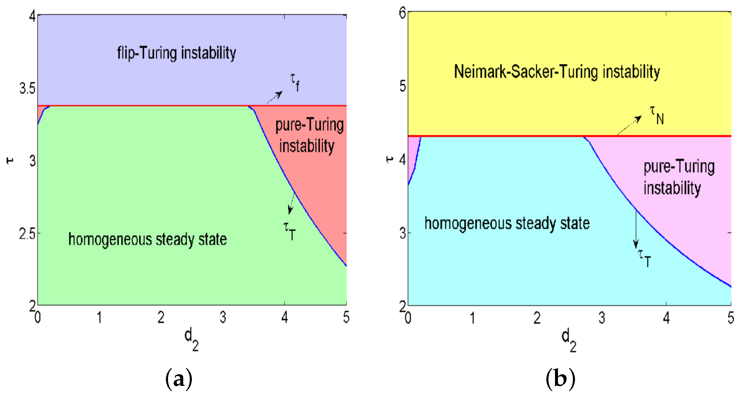
3.3. Turing Bifurcation

Assume that one of ($H1$)–($H2$) holds. For Turing bifurcation, the eigenvalues for the discrete Laplacian operator ${\Delta }_d$ should be studied in this part. Hence, the characteristic equation for ${\Delta }_d$ is defined by

$$\begin{array}{c}\hfill {\Delta }_d{X}^{i,j}+\lambda X^{i,j}=0,\end{array}$$

(27)

with periodic boundary conditions

$$X^{i,0}=X^{i,n},X^{i,1}=X^{i,n+1},X^{0,j}=X^{n,j},X^{1,j}=X^{n+1,j},i,j\in 1,2,\cdots ,n.$$

In [31], one knows that the discrete Laplacian operator ${\Delta }_d$ has the following forms eigenvalues

$${\lambda }_{kl}=4(si{n}^2{\varphi }_k+si{n}^2{\varphi }_l),$$

where ${\varphi }_k=\frac{(k-1)\pi }{n},{\varphi }_l=\frac{(l-1)\pi }{n}$ and $k,l\in \{1,2,3,\cdots ,n\}.$

Let $\tilde{a}(i,j,t)=a(i,j,t)-a_{\ast }$ and $\tilde{h}(i,j,t)=h(i,j,t)-h_{\ast }$, and notice that ${\Delta }_d\tilde{a}(i,j,t)={\Delta }_{d}a(i,j,t)$ and ${\Delta }_d\tilde{h}(i,j,t)={\Delta }_{d}h(i,j,t)$, and taking this transformation into Equations (4)–(7), one has

$$\begin{array}{c}\hfill \left(\begin{array}{c}{\tilde{a}}_{i,j,t+1}\\ {\tilde{h}}_{i,j,t+1}\end{array}\right)=\left(\begin{array}{cc}{a}_{10}& a_{01}\\ b_{10}& b_{01}\end{array}\right)\left(\begin{array}{c}{\tilde{a}}_{i,j,t}\\ {\tilde{h}}_{i,j,t}\end{array}\right)+\left(\begin{array}{c}{a}_{10}\frac{\tau }{{\delta }^2}{d}_1{\Delta }_d{\tilde{a}}_{i,j,t}+a_{01}\frac{\tau }{{\delta }^2}{d}_2{\Delta }_d{\tilde{h}}_{i,j,t}+\mathcal{O}\left(2\right)\\ b_{10}\frac{\tau }{{\delta }^2}{d}_1{\Delta }_d{\tilde{a}}_{i,j,t}+b_{01}\frac{\tau }{{\delta }^2}{d}_2{\Delta }_d{\tilde{h}}_{i,j,t}+\mathcal{O}\left(2\right)\end{array}\right),\end{array}$$

(28)

where $a_{10},a_{01},b_{10},b_{01}$ are defined in above analysis. If the perturbations are small, the higher order terms can be omitted.

Assume that $X_{kl}^{ij}$ as the eigenfunction of the eigenvalues ${\lambda }_{kl}$, and multiplying the both sides of Equation (28) by $X_{kl}^{ij}$, one gets

$$\begin{array}{c}\hfill \left(\begin{array}{c}{X}_{kl}^{ij}{\tilde{a}}_{i,j,t+1}\\ X_{kl}^{ij}{\tilde{h}}_{i,j,t+1}\end{array}\right)=\left(\begin{array}{cc}{a}_{10}& a_{01}\\ b_{10}& b_{01}\end{array}\right)\left(\begin{array}{c}{X}_{kl}^{ij}{\tilde{a}}_{i,j,t}\\ X_{kl}^{ij}{\tilde{h}}_{i,j,t}\end{array}\right)+\left(\begin{array}{c}{a}_{10}\frac{\tau }{{\delta }^2}{X}_{kl}^{ij}{d}_1{\Delta }_d{\tilde{a}}_{i,j,t}+a_{01}\frac{\tau }{{\delta }^2}{X}_{kl}^{ij}{d}_2{\Delta }_d{\tilde{h}}_{i,j,t}\\ b_{10}\frac{\tau }{{\delta }^2}{X}_{kl}^{ij}{d}_1{\Delta }_d{\tilde{a}}_{i,j,t}+b_{01}\frac{\tau }{{\delta }^2}{X}_{kl}^{ij}{d}_2{\Delta }_d{\tilde{h}}_{i,j,t}\end{array}\right).\end{array}$$

(29)

Summing Equation (29) for all of i and j, one obtains that

$$\begin{array}{cc}\hfill \left(\begin{array}{c}\sum X_{kl}^{ij}{\tilde{a}}_{i,j,t+1}\\ \sum X_{kl}^{ij}{\tilde{h}}_{i,j,t+1}\end{array}\right)& =\left(\begin{array}{cc}{a}_{10}& a_{01}\\ b_{10}& b_{01}\end{array}\right)\left(\begin{array}{c}\sum X_{kl}^{ij}{\tilde{a}}_{i,j,t}\\ \sum X_{kl}^{ij}{\tilde{h}}_{i,j,t}\end{array}\right)\hfill \\ \hfill & +\left(\begin{array}{c}{a}_{10}\frac{\tau }{{\delta }^2}\sum X_{kl}^{ij}{d}_1{\Delta }_d{\tilde{a}}_{i,j,t}+a_{01}\frac{\tau }{{\delta }^2}\sum X_{kl}^{ij}{d}_2{\Delta }_d{\tilde{h}}_{i,j,t}+\mathcal{O}\left(2\right)\\ b_{10}\frac{\tau }{{\delta }^2}\sum X_{kl}^{ij}{d}_1{\Delta }_d{\tilde{a}}_{i,j,t}+b_{01}\frac{\tau }{{\delta }^2}\sum X_{kl}^{ij}{d}_2{\Delta }_d{\tilde{h}}_{i,j,t}+\mathcal{O}\left(2\right)\end{array}\right).\hfill \end{array}$$

(30)

Let ${\overline{a}}_{t+1}=\sum X_{kl}^{ij}{\tilde{a}}_{i,j,t+1},{\overline{h}}_{t+1}=\sum X_{kl}^{ij}{\tilde{h}}_{i,j,t+1},$ hence, (30) becomes

$$\begin{array}{c}\hfill \left(\begin{array}{c}{\overline{a}}_{t+1}\\ {\overline{h}}_t\end{array}\right)=\left(\begin{array}{cc}{a}_{10}& a_{01}\\ b_{10}& b_{01}\end{array}\right)\left(\begin{array}{c}{\overline{a}}_t\\ {\overline{h}}_t\end{array}\right)+\left(\begin{array}{c}{a}_{10}(-\frac{\tau }{{\delta }^2}{d}_1{\lambda }_{kl}){\overline{a}}_t+a_{01}(-\frac{\tau }{{\delta }^2}{d}_2{\lambda }_{kl}){\overline{h}}_t+\mathcal{O}\left(2\right)\\ b_{10}(-\frac{\tau }{{\delta }^2}{d}_1{\lambda }_{kl}){\overline{a}}_t+b_{01}(-\frac{\tau }{{\delta }^2}{d}_2{\lambda }_{kl}){\overline{h}}_t+\mathcal{O}\left(2\right)\end{array}\right).\end{array}$$

(31)

Hence, the eigenvalues of the Jacobian of equations of system (31) are

$$\begin{array}{c}\hfill {\lambda }_{\pm }(k,l,\tau )=\frac{1}{2}{P}_T(k,l,\tau )\pm \frac{1}{2}\sqrt{P_T{(k,l,\tau )}^2-4Q_T(k,l,\tau )},\end{array}$$

(32)

where

$$\begin{array}{cc}\hfill P_T(k,l,\tau )& =-p\left(\tau \right)-\frac{\tau }{{\delta }^2}(a_{10}\left(\tau \right)d_1+b_{01}\left(\tau \right)d_2){\lambda }_{kl},\hfill \\ \hfill Q_T(k,l,\tau )& =q\left(\tau \right)(1-\frac{\tau }{{\delta }^2}{d}_1{\lambda }_{kl})(1-\frac{\tau }{{\delta }^2}{d}_2{\lambda }_{kl}).\hfill \end{array}$$

In addition, one defines

$$\begin{array}{c}\hfill Z_T(k,l,\tau )=max\left(\right|{\lambda }_{+}(k,l,\tau )|,|{\lambda }_{-}(k,l,\tau )\left|\right),\end{array}$$

(33)

$$\begin{array}{c}\hfill Z_m\left(\tau \right)=\underset{k=1,l=1}{\overset{n}{max}}{Z}_T(k,l,\tau ),((k,l)\ne (1,1)).\end{array}$$

(34)

$Z_m\left(\tau \right)=1$ is the threshold condition for the occurrence of Turing bifurcation. In addition, if $P_T{(k,l,\tau )}^2-4Q_T(k,l,\tau )>0$ holds, the critical value ${\tau }_T$ satisfies

$$\begin{array}{c}\hfill \underset{k=1,l=1}{\overset{n}{max}}\left(\right|P_T(k,l,\tau )|-Q_T(k,l,\tau ))=1;\end{array}$$

(35)

if $P_T{(k,l,\tau )}^2-4Q_T(k,l,\tau )\le 0$ holds, the critical value ${\tau }_T$ satisfies

$$\begin{array}{c}\hfill \underset{k=1,l=1}{\overset{n}{max}}{Q}_T(k,l,\tau )=1.\end{array}$$

(36)

Theorem 3.

Assume that one of ($H1$)–($H5$) holds, and τ is close to ${\tau }_T$. If $Z_m\left(\tau \right)>1$, the homogeneous steady state of model (3) with periodic conditions undergo Turing instability, and Turing patterns will occur. If $Z_m\left(\tau \right)<1$, the homogeneous steady state is still stable; no Turing patterns will occur.

4. Numerical Simulations

In this section, we will give some examples to illustrate the results in Section 3. We can find the bifurcations and chaos, as well as many different Turing patterns in this part by numerical simulations.

4.1. The Dynamics Behaviors for Spatially Homogeneous State

In this sunsection, we show the temporal dynamics of flip bifurcation and Neimark–Sacker bifurcation. Let $c=0.5,\mu =0.2015$, then the positive equilibrium is $(a_{\ast },h_{\ast })=(7.4442,55.4156)$ and critical value for flip bifurcation is ${\tau }_f=3.37221.$$c=0.5,\mu =0.2156$, then the positive equilibrium is $(a_{\ast },h_{\ast })=(6.9573,48.4044)$, and the critical value for Neimark–Sacker bifurcation is ${\tau }_N=4.304889.$

Moreover, the flip bifurcation diagram, Neimark–Sacker bifurcation diagram and the corresponding maximum Lyapunov exponents are shown in Figure 1 and Figure 2, respectively. Besides, the phase orbits for flip bifurcation and Neimark–Sacker bifurcation are shown in Figure 3 and Figure 4, respectively.

From Figure 3, we can see that there exists stable periodic—2, 4, 8, 10 points as $\tau$ great than ${\tau }_f$ sightly, as shown in Figure 3a–c,e, respectively. We can also find chaos (Figure 3d,f) as $\tau$ increases furthermore.

From Figure 4, we can see that there exists a stable limit cycle as $\tau$ great than ${\tau }_N$ sightly, as shown in Figure 4a. We can also find chaos (Figure 4c) as $\tau$ increases furthermore. During the route to chaos, we find that there exists periodic-11 windows, as shown in Figure 4b.

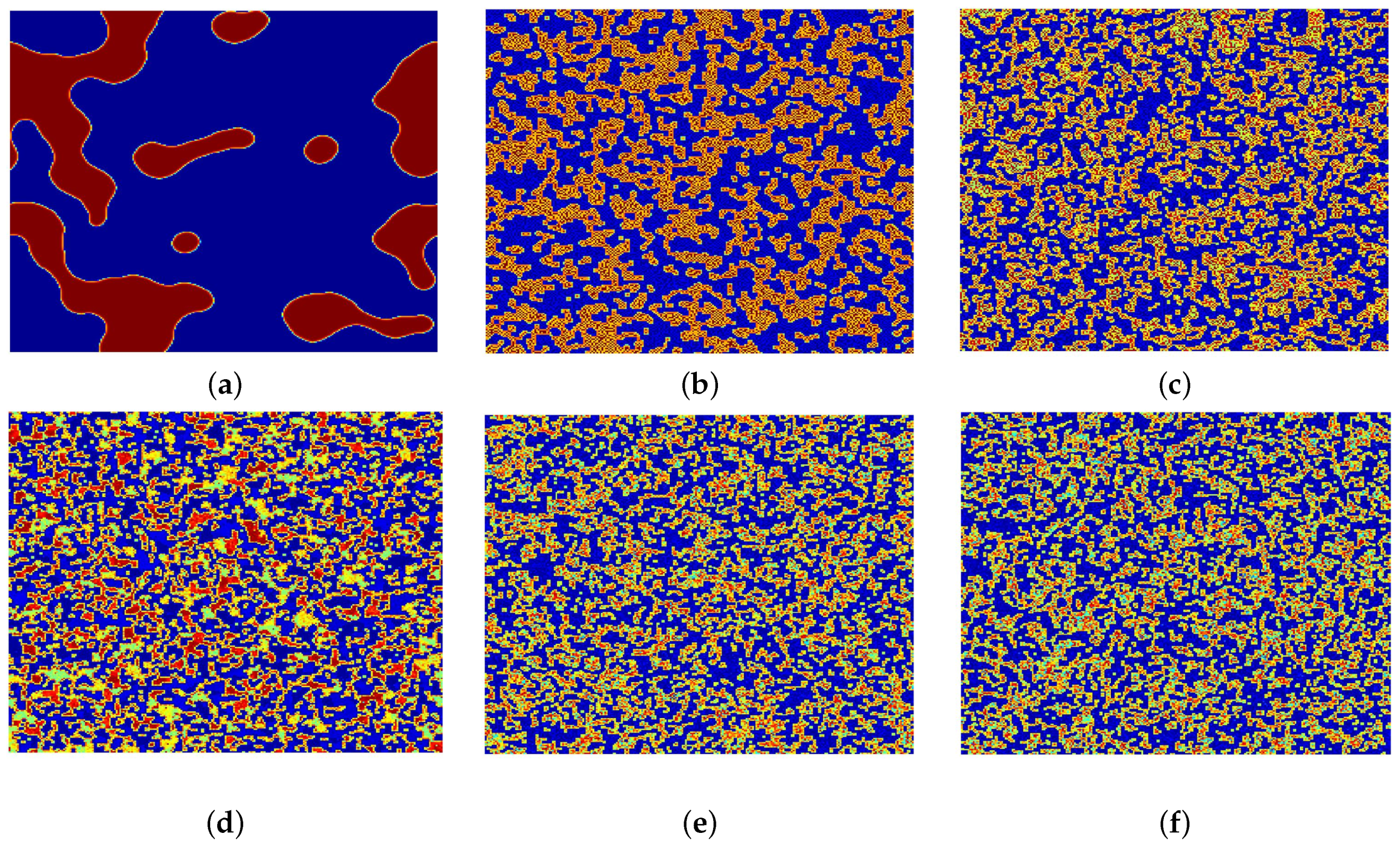
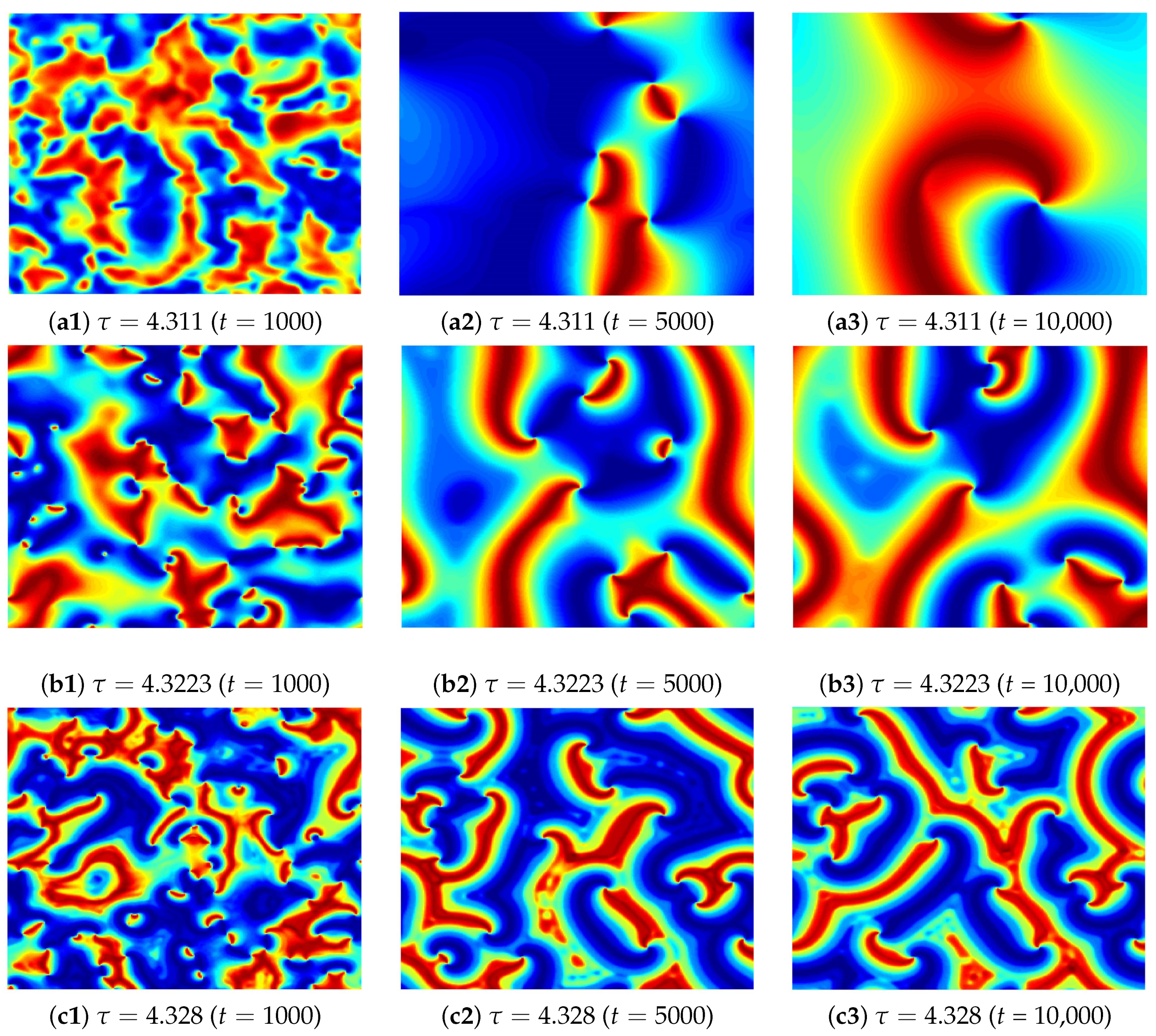
4.2. The Dynamics Behaviors for Spatially Heterogenous State

In this part, we show the spatiotemporally dynamics of Turing instability for flip bifurcation and Neimark–Sacker bifurcation. In order to ensure that a and h are non-negative, we need $d_i\Delta t(\frac{1}{{(\Delta x)}^2}+\frac{1}{{(\Delta x)}^2})<0.5$, $i=1,2$. Let $d_1=0.2$ and $n=256$; the $Z_m-\tau$ diagrams are shown in Figure 5. We find that Turing bifurcation curve $\tau ={\tau }_T$ and the flip bifurcation curve $\tau ={\tau }_f$ (or Neimark–Sacker bifurcation curve $\tau ={\tau }_N$) divide parametric space, $(d_2,\tau )$, into three regions, as shown in Figure 3a (or Figure 3b). Moreover, Let $d_2=0.5$; we can observe that the critical value for Turing instability in flip bifurcation and Neimark–Sacker bifurcation are ${\tau }_T=3.37221$ and ${\tau }_T=4.304886$, respectively.

In this sequel, we show the patterns for flip-Turing instability. Let $\tau =3.6$; the pattern induced by periodic-2 points [27,31] is shown in Figure 6a, which is formed by two alteration states. Similarly, taking $\tau =3.8$ and $\tau =3.96$, the patterns induced by periodic-4 and -8 points are shown in Figure 6b,c, respectively. Besides, on the paths to chaos, there exists a pattern induced by periodic-10 points, which is shown in Figure 6e. Taking $\tau =4.02$ and $\tau =4.18$, the patterns induced by chaotic attractors are shown in Figure 6d,f, respectively. It is clear to observe that the pattern in Figure 6f is more fragmented than that one in Figure 6d, which means that the self-organized symmetric patterns are broken and spatial chaotic characteristics are shown.

In this sequel, we show the patterns for Neimark–Sacker Turing instability. Let $\tau =4.11$, the pattern induced by invariant circles, be shown in Figure 7(a1–a3) for $t=1000,$t=5000, and t = 10,000, respectively. As $\tau$ increases to 4.3223 continuously, the circular pattern induced by periodic-11 orbit is shown in Figure 7(b1–b3) for $t=1000,t=5000$, and t = 10,000, respectively, which is more twisted than the top patterns of Figure 7. As $\tau$ reaches to 4.328 eventually, the pattern induced by the homogeneous chaotic oscillating states [27,31] are more twisted than the former two, as shown in Figure 7(c1–c3) for $t=1000,$$t=5000$, and t = 10,000, respectively,

5. Conclusions and Future Direction

The flip, Neimark–Sacker and Turing bifurcations of a spatiotemporal discrete Gierer-Meinhardt system are investigated in this paper. In addition, we illustrate the patterns induced by the flip-Turing and Neimark–Sacker Turing instability. Compared to the previous works [3,34], we found that the flip-Turing patterns and Neimark–Sacker–Turing patterns are similar with the patterns induced by the real Ginzburg–Landau equation which emerges as the amplitude equation near a Hopf instability to a continuous reaction–diffusion system, such as the defect turbulence. In fact, the coupled map lattice system is a dynamic system that discretizes time and space but its state variables still remain continuous. Hence, what is the relationship between the patterns of a continuous reaction–diffusion system and a spatiotemporal discrete one? It is worth investigating this phenomenon in further work.

References

1. Turing, A. The chemical basis of morphogenesis. Philos. Trans. R. Soc. Bull. Biol. Sci. 1952, 237, 37–72. [Google Scholar]
2. Han, Y.; Han, B.; Zhang, L.; Xu, L.; Li, M.F.; Zhang, G. Turing instability and wave patterns for a symmetric discrete competitive Lotka-Volterra system. WSEAS Trans. Math. 2011, 10, 181–189. [Google Scholar]
3. Liu, B.; Wu, R.; Chen, L. Turing-Hopf bifurcation analysis in a superdiffusive predator-prey model. Chaos 2018, 28, 113118. [Google Scholar] [CrossRef]
4. Liu, B.; Wu, R.; Iqbal, N.; Chen, L. Turing patterns in the Lengyel-Epstein system with superdiffusion. Int. J. Bifurcat. Chaos 2017, 27, 1730026. [Google Scholar] [CrossRef]
5. Iqbal, N.; Wu, R.; Liu, B. Pattern formation by super-diffusion in FitzHugh-Nagumo model. Appl. Math. Comput. 2017, 313, 245–258. [Google Scholar] [CrossRef]
6. Gierer, A.; Meinhardt, H. A theory of biological pattern formation. Kybernetik 1972, 12, 30–39. [Google Scholar] [CrossRef] [Green Version]
7. Ward, M.J.; Wei, J. Hopf bifurcations and oscillatory instabilities of spike solutions for the one-dimensional Gierer-Meinhardt model. J. Nonlinear Sci. 2003, 13, 209–264. [Google Scholar] [CrossRef]
8. Wei, J.; Winter, M. On the two-dimensional Gierer-Meinhardt system with strong coupling. SIAM J. Math. Anal. 1999, 30, 1241–1263. [Google Scholar] [CrossRef]
9. Ruan, S. Diffusion-driven instability in the Gierer-Meinhardt model of morphogenesis. Nat. Resour. Model. 1998, 11, 131–141. [Google Scholar] [CrossRef]
10. Wang, J.; Hou, X.; Jing, Z. Stripe and spot patterns in a Gierer-Meinhardt activator-inhibitor model with different sources. Int. J. Bifuru. Chaos 2015, 25, 1550108. [Google Scholar] [CrossRef]
11. Mai, F.; Qin, L.; Zhang, G. Turing instability for a semi-discrete Gierer-Meinhardt system. Physica A 2012, 391, 2014–2022. [Google Scholar] [CrossRef]
12. Wang, J.; Li, Y.; Zhong, S.; Hou, X. Analysis of bifurcation, chaos and pattern formation in a discrete time and space Gierer Meinhardt system. Chaos Solitons Fract. 2019, 118, 1–17. [Google Scholar] [CrossRef]
13. Liu, J.; Yi, F.; Wei, J. Multiple bifurcation analysis and spatiotemporal patterns in a 1-D Gierer-Meinhardt model of morphogenesis. Int. J. Bifuru. Chaos 2010, 20, 1007–1025. [Google Scholar] [CrossRef]
14. Li, Y.; Wang, J.; Hou, X. Stripe and spot patterns for the Gierer-Meinhardt model with saturated activator production. J. Math. Anal. Appl. 2017, 449, 1863–1879. [Google Scholar] [CrossRef]
15. Wu, R.; Zhou, Y.; Shao, Y.; Chen, L. Bifurcation and Turing patterns of reaction-diffusion activator-inhibitor model. Physica A 2017, 482, 597–610. [Google Scholar] [CrossRef]
16. Lee, S.S.; Gaffney, E.; Monk, N. The influence of gene expression time delays on Gierer-Meinhardt pattern formation systems. Bull. Math. Biol. 2010, 72, 2139–2160. [Google Scholar]
17. Wei, J.; Yang, W. Multi-bump ground states of the fractional Gierer-Meinhardt system on the real line. J. Dyn. Diff. Equ. 2019, 31, 385–417. [Google Scholar] [CrossRef]
18. Domokos, G.; Scheuring, I. Discrete and continuous state population models in a noisy world. J. Theor. Biol. 2004, 227, 535–545. [Google Scholar] [CrossRef] [Green Version]
19. Koch, A.J.; Meinhardt, H. Biological pattern formation: From basic mechanisms to complex structures. Rev. Mod. Phys. 1994, 66, 1481. [Google Scholar] [CrossRef]
20. Meinhardt, H. Models of Biological Pattern Formation; Academic Press: Cambridge, MA, USA, 1982. [Google Scholar]
21. Meinhardt, H. The Algorithmic Beauty of Sea Shells; Springer Science & Business Media: Berlin/Heidelberg, Germany, 2009. [Google Scholar]
22. Punithan, D.; Kim, D.K.; McKay, R. Spatio-temporal dynamics and quantification of daisyworld in two-dimensional coupled map lattices. Ecol. Complex. 2012, 12, 43–57. [Google Scholar] [CrossRef]
23. Jing, Z.; Yang, J. Bifurcation and chaos in discrete-time predator-prey system. Chaos Solitons Fract. 2006, 27, 259–277. [Google Scholar] [CrossRef]
24. Liu, X.; Xiao, D. Complex dynamic behaviors of a discrete-time predator-prey system. Chaos Solitons Fract. 2007, 32, 80–94. [Google Scholar] [CrossRef]
25. Rodrigues, L.A.D.; Mistro, D.C.; Petrovskii, S. Pattern formation in a space- and time-discrete predator-prey system with a strong allee effect. Theor. Ecol. 2011, 5, 341–362. [Google Scholar] [CrossRef]
26. Bai, L.; Zhang, G. Nontrivial solutions for a nonlinear discrete elliptic equation with periodic boundary conditions. Appl. Math. Comput. 2009, 210, 321–333. [Google Scholar] [CrossRef]
27. Zhong, S.; Wang, J.; Li, Y.; Jiang, N. Bifurcation, chaos and Turing instability analysis for a space-time discrete toxic phytoplankton-zooplankton model with self-diffusion, Internat. J. Bifurc. Chaos 2019, 29, 1950184. [Google Scholar] [CrossRef]
28. Zhong, S.; Wang, J.; Bao, J.; Li, Y.; Jiang, N. Spatiotemporal complexity analysis for a space-time discrete generalized toxic-phytoplankton-zooplankton model with self-diffusion and cross-diffusion. Internat. J. Bifurc. Chaos 2021, 31, 2150006. [Google Scholar] [CrossRef]
29. Zhang, F.; Zhou, W.; Yao, L.; Li, Y.; Jiang, N. Spatiotemporal patterns formed by a discrete nutrient-phytoplankton model with time delay. Complexity 2020, 31, 8541432. [Google Scholar] [CrossRef]
30. Nakata, K.; Sokabe, M.; Suzuki, R. The application of the Gierer-Meinhardt equations to the development of the retinotectal projection. Biol. Cybern. 1979, 35, 235–241. [Google Scholar] [CrossRef]
31. Huang, T.; Zhang, H. Chaos and pattern formation in a space- and time-discrete predator-prey system. Chaos Solitons Fract. 2016, 91, 92–107. [Google Scholar] [CrossRef]
32. Wiggins, S. Introduction to Applied Nonlinear Dynamical Systems and Chaos, 2nd ed.; Spring Science + Business Media, LLC.: Berlin/Heidelberg, Germany, 1990; pp. 193–381. [Google Scholar]
33. Guckenheimer, J.; Holmes, P. Nonlinear Oscillations, Dynamical Systems, and Bifurcations of Vector Fields; Spring: Berlin/Heidelberg, Germany, 1983; pp. 117–165. [Google Scholar]
34. Torabi, R.; Rezaei, Z. Instability in reaction-superdiffusion systems. Phys. Rev. E 2016, 94, 052202. [Google Scholar] [CrossRef] [Green Version]
Figure 1. (a) Flip bifurcation diagram; (b) Maximum Lyapunov exponents.
Mathematics 10 00243 g001
Figure 2. (a) Neimark-Sacker bifurcation diagram; (b) Maximum Lyapunov exponents.
Mathematics 10 00243 g002
Figure 3. Phase portraits for different values of τ corresponding to Figure 1a. (a) τ = 3.6 ; (b) τ = 3.8 ; (c) τ = 3.96 ; (d) τ = 4.02 ; (e) τ = 4.12 ; (f) τ = 4.18 .
Mathematics 10 00243 g003
Figure 4. Phase portraits for different values of τ corresponding to Figure 3a. (a) τ = 4.311 ; (b) τ = 4.3223 ; (c) τ = 4.328 .
Mathematics 10 00243 g004
Figure 5. (a) Z m τ diagram for Turing instability in flip bifurcation; (b) Z m τ diagram for Turing instability in Neimark–Sacker bifurcation.
Mathematics 10 00243 g005
Figure 6. The patterns for flip-Turing instability. (a) τ = 3.6 ; (b) τ = 3.8 ; (c) τ = 3.96 ; (d) τ = 4.02 ; (e) τ = 4.12 ; (f) τ = 4.18 .
Mathematics 10 00243 g006
Figure 7. The patterns for Neimark-Sacker Turing instability.
Mathematics 10 00243 g007
Publisher’s Note: MDPI stays neutral with regard to jurisdictional claims in published maps and institutional affiliations.