Figure 1.
Example of domain split in four subdomains with overlap.
Figure 1.
Example of domain split in four subdomains with overlap.
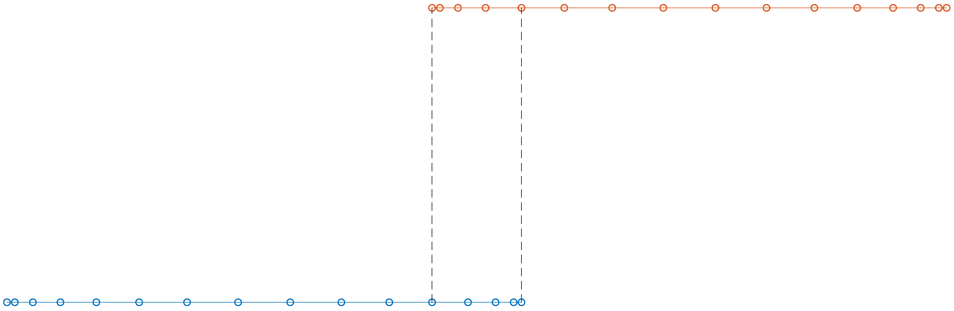
Figure 2.
Example of overlap between Legendre collocation nodes in adjacent domains; , overlap = 4.
Figure 2.
Example of overlap between Legendre collocation nodes in adjacent domains; , overlap = 4.
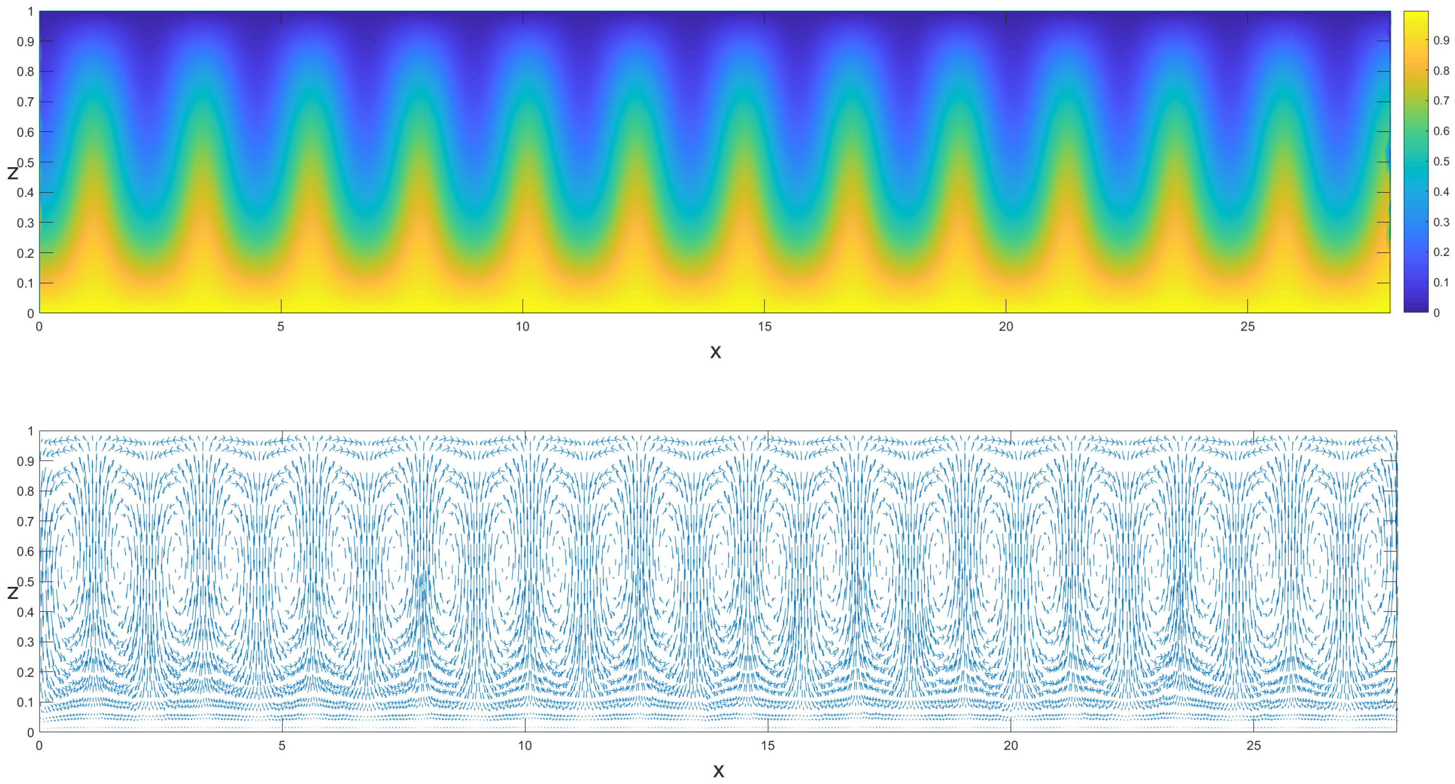
Figure 3.
Isotherms and velocity field of the numerical solution obtained with finite elements; and .
Figure 3.
Isotherms and velocity field of the numerical solution obtained with finite elements; and .
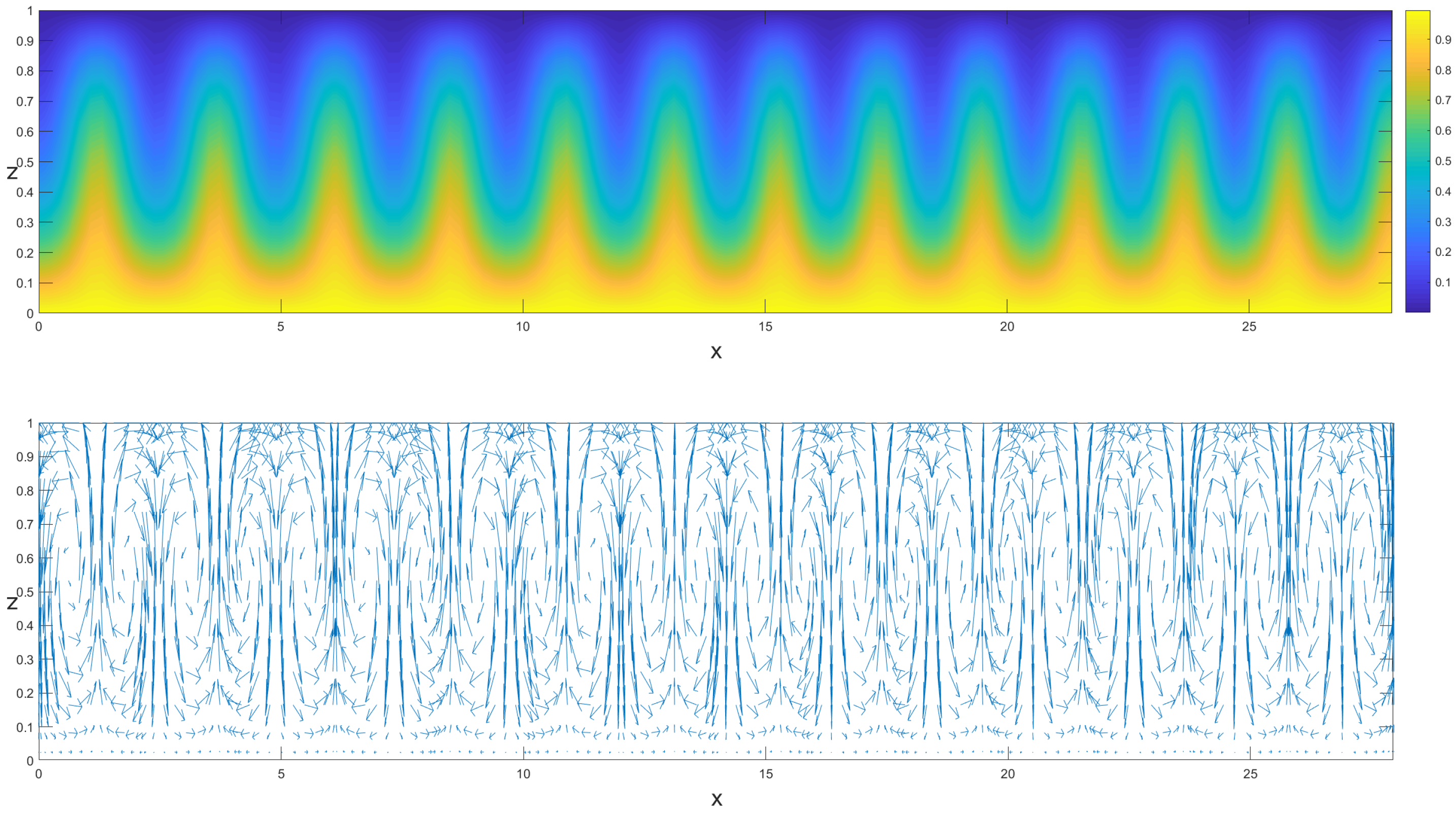
Figure 4.
Isotherms and velocity field of the numerical solution obtained with alternating Schwarz; and .
Figure 4.
Isotherms and velocity field of the numerical solution obtained with alternating Schwarz; and .
Figure 5.
Isotherms and velocity field of the numerical solution obtained with finite elements; and .
Figure 5.
Isotherms and velocity field of the numerical solution obtained with finite elements; and .
Figure 6.
Isotherms and velocity field of the numerical solution obtained with alternating Schwarz; and .
Figure 6.
Isotherms and velocity field of the numerical solution obtained with alternating Schwarz; and .
Figure 7.
Isotherms and velocity field of the numerical solution obtained with finite elements; and .
Figure 7.
Isotherms and velocity field of the numerical solution obtained with finite elements; and .
Figure 8.
Isotherms and velocity field of the numerical solution obtained with alternating Schwarz; and .
Figure 8.
Isotherms and velocity field of the numerical solution obtained with alternating Schwarz; and .
Figure 9.
Isotherms and velocity field of the numerical solution obtained with finite elements; and .
Figure 9.
Isotherms and velocity field of the numerical solution obtained with finite elements; and .
Figure 10.
Isotherms and velocity field of the numerical solution obtained with alternating Schwarz; and .
Figure 10.
Isotherms and velocity field of the numerical solution obtained with alternating Schwarz; and .
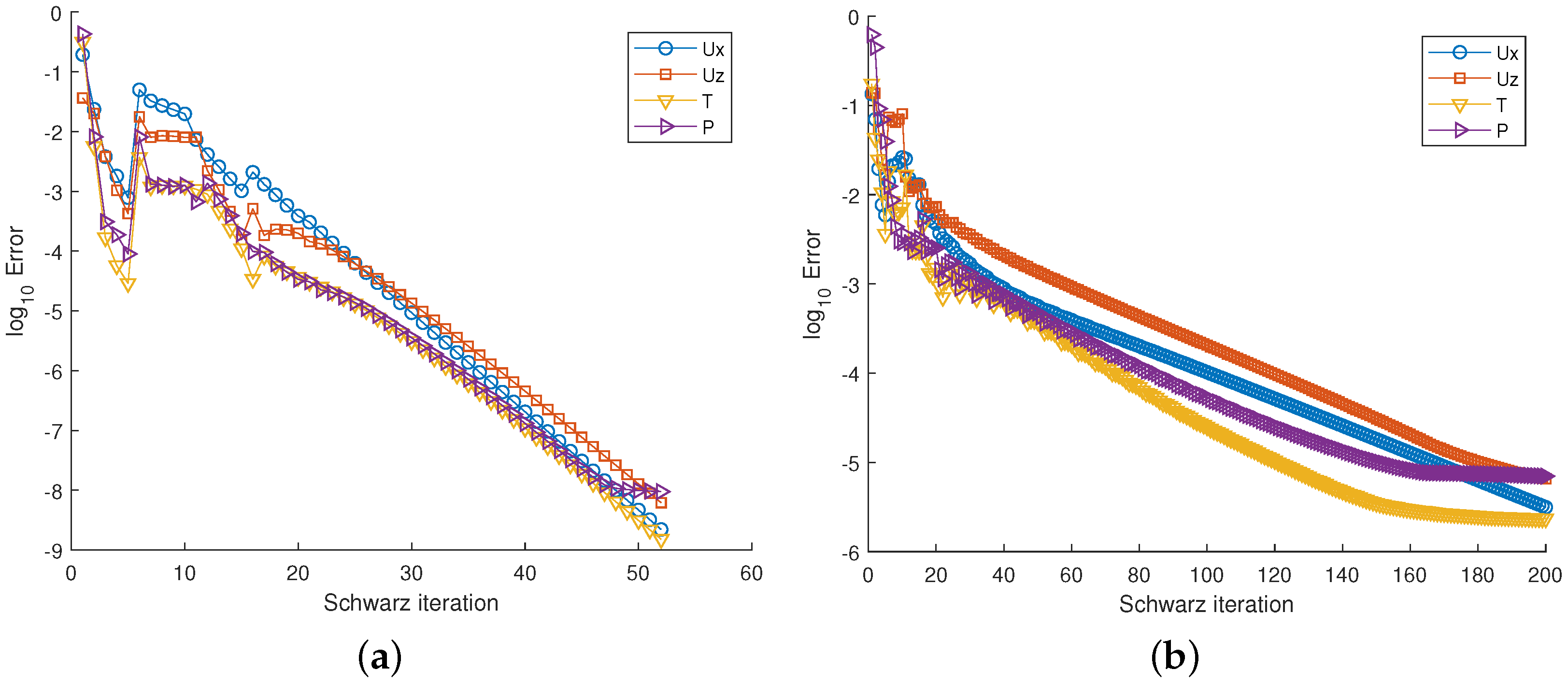
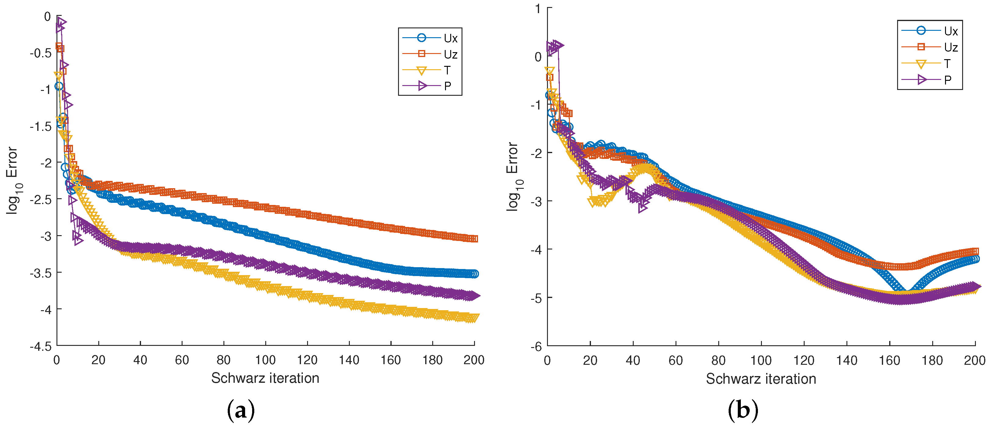
Figure 11.
Graph of the log of the errors in the velocity, temperature, and pressure fields for the Schwarz iterations: (a) , , , , ; (b) , , , , .
Figure 11.
Graph of the log of the errors in the velocity, temperature, and pressure fields for the Schwarz iterations: (a) , , , , ; (b) , , , , .
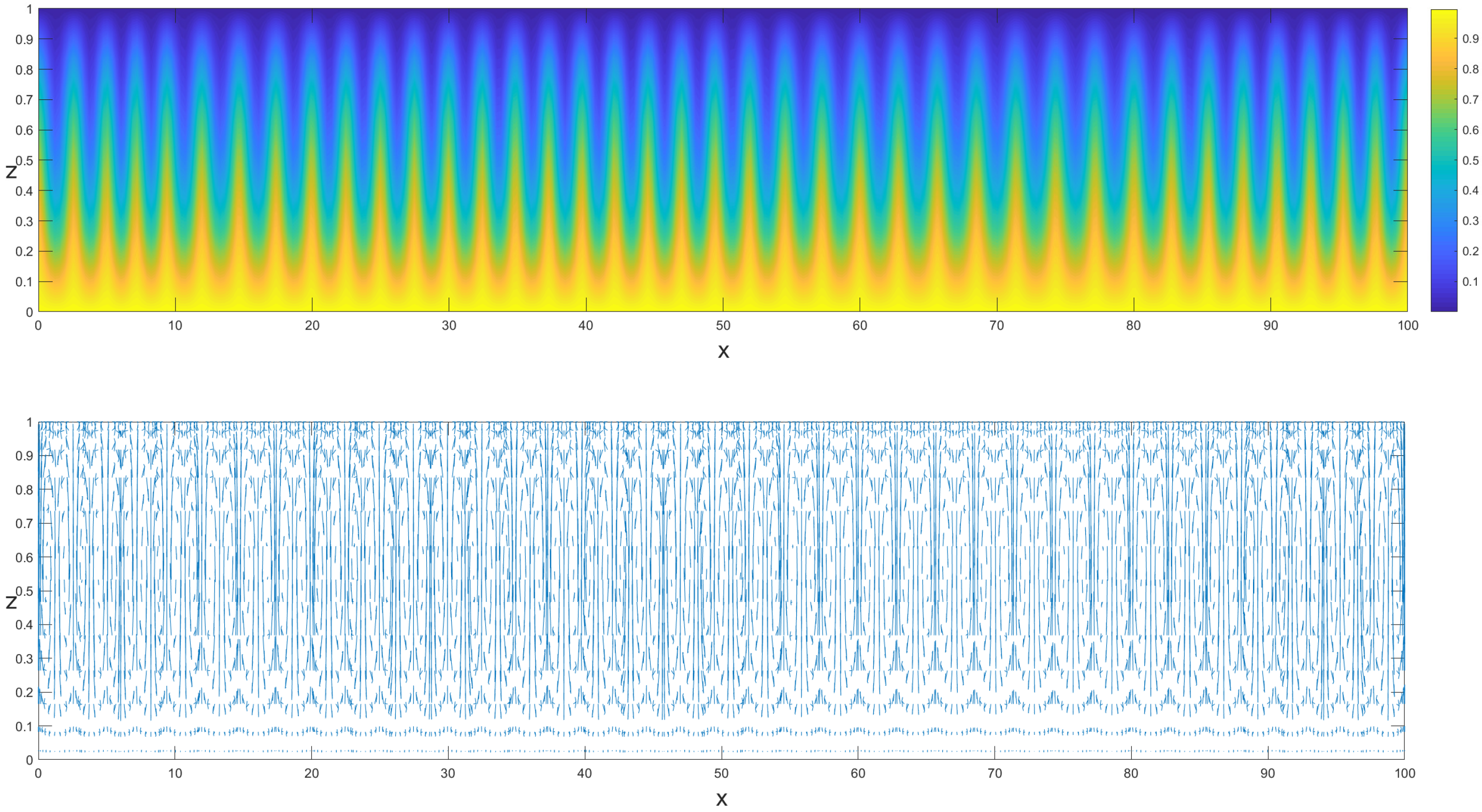
Figure 12.
Isotherms and velocity field of a numerical solution obtained with alternating Schwarz domain decomposition; , , , , .
Figure 12.
Isotherms and velocity field of a numerical solution obtained with alternating Schwarz domain decomposition; , , , , .
Figure 13.
Isotherms and velocity field of a numerical solution obtained with alternating Schwarz domain decomposition; , , , , .
Figure 13.
Isotherms and velocity field of a numerical solution obtained with alternating Schwarz domain decomposition; , , , , .
Figure 14.
Graph of the log of the errors in the velocity, temperature, and pressure fields for the Schwarz iterations: (a) , , , , ; (b) , , , , .
Figure 14.
Graph of the log of the errors in the velocity, temperature, and pressure fields for the Schwarz iterations: (a) , , , , ; (b) , , , , .
Figure 15.
Graph of the log of the errors in the velocity, temperature, and pressure fields for the Schwarz iterations: (a) , , , , ; (b) , , , , .
Figure 15.
Graph of the log of the errors in the velocity, temperature, and pressure fields for the Schwarz iterations: (a) , , , , ; (b) , , , , .
Figure 16.
Isotherms and velocity field of a numerical solution obtained with alternating Schwarz domain decomposition; , , , , .
Figure 16.
Isotherms and velocity field of a numerical solution obtained with alternating Schwarz domain decomposition; , , , , .
Figure 17.
Isotherms and velocity field of a numerical solution obtained with alternating Schwarz domain decomposition; , , , , .
Figure 17.
Isotherms and velocity field of a numerical solution obtained with alternating Schwarz domain decomposition; , , , , .
Figure 18.
(a) Convergence rate for the Schwarz iterations: , ; (b) convergence rate for the Schwarz iterations: , .
Figure 18.
(a) Convergence rate for the Schwarz iterations: , ; (b) convergence rate for the Schwarz iterations: , .
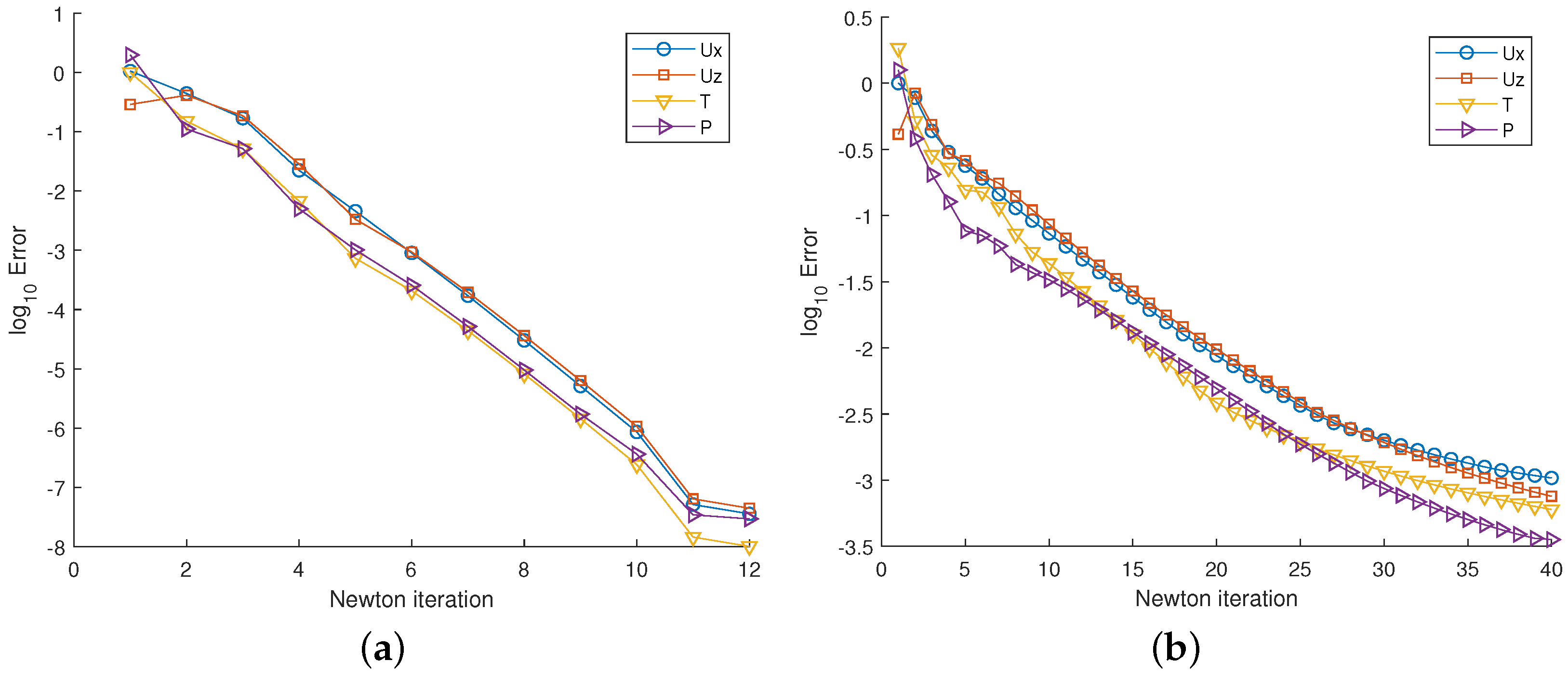
Figure 19.
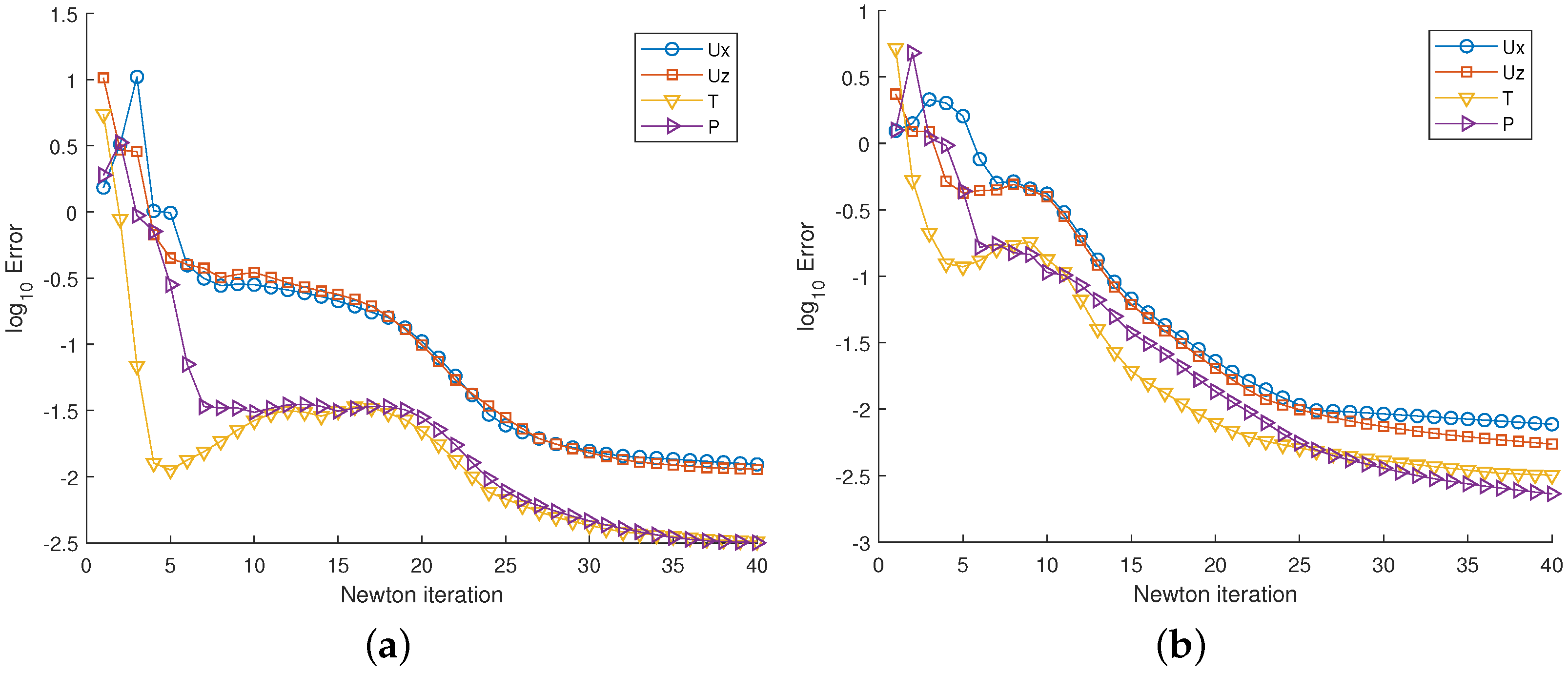
Graph of the log of the errors in the velocity, temperature, and pressure fields for the Newton iterations: (a) , , , , ; (b) , , , , .
Figure 19.
Graph of the log of the errors in the velocity, temperature, and pressure fields for the Newton iterations: (a) , , , , ; (b) , , , , .
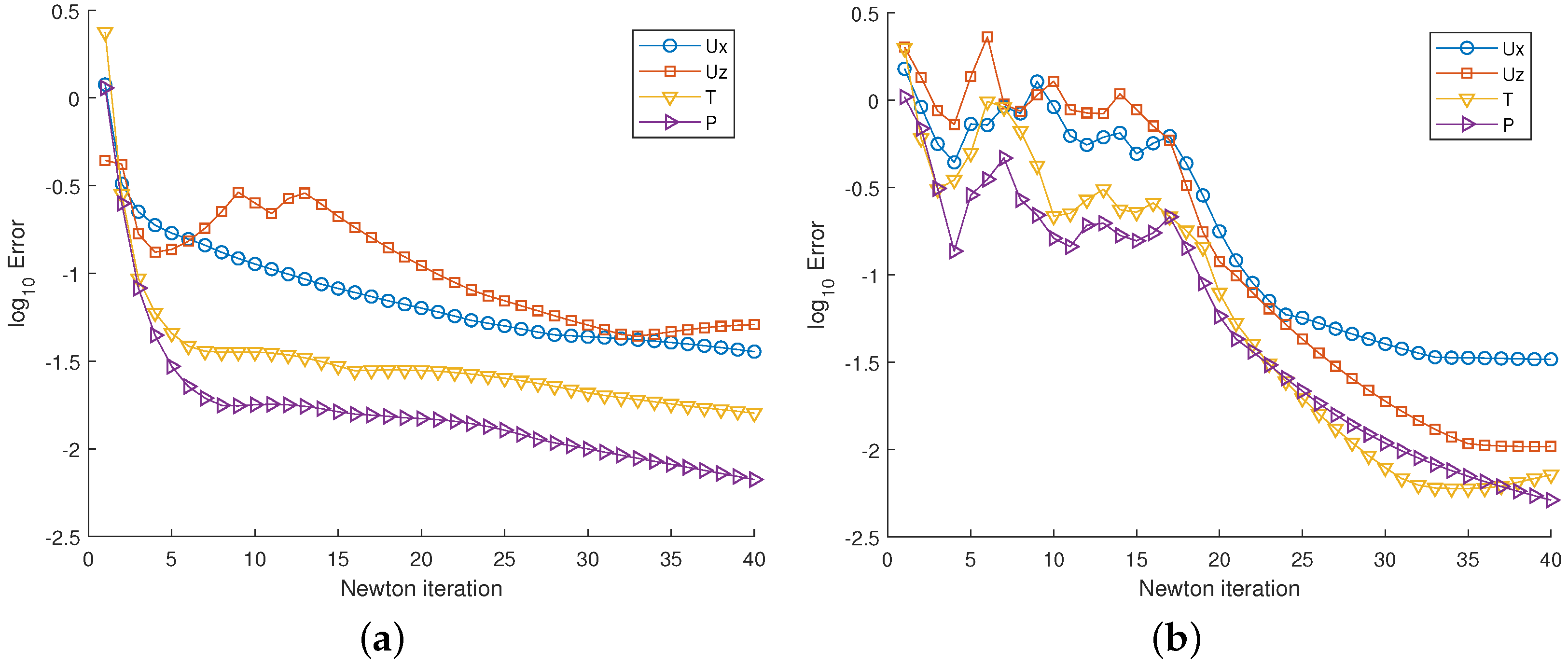
Figure 20.
Graph of the log of the errors in the velocity, temperature, and pressure fields for the Newton iterations: (a) , , , , ; (b) , , , , .
Figure 20.
Graph of the log of the errors in the velocity, temperature, and pressure fields for the Newton iterations: (a) , , , , ; (b) , , , , .
Figure 21.
Graph of the log of the errors in the velocity, temperature, and pressure fields for the Newton iterations: (a) , , , , ; (b) , , , , .
Figure 21.
Graph of the log of the errors in the velocity, temperature, and pressure fields for the Newton iterations: (a) , , , , ; (b) , , , , .
Figure 22.
Ratio of the convergence of the Newton’s method for , , , , .
Figure 22.
Ratio of the convergence of the Newton’s method for , , , , .
Figure 23.
Ratio of the convergence of the Newton’s method for , , , , .
Figure 23.
Ratio of the convergence of the Newton’s method for , , , , .
Table 1.
Relative norm of the difference between the horizontal component of the velocity solution, , obtained with Legendre collocation with a mesh in a single domain and the solution obtained with different numbers of subdomains on the horizontal axis, , a single domain on the vertical axis, , and different Legendre collocation meshes ; and .
| np | | | | |
|---|
| 1 | 1.2559 | 0.0324 | 0.0128 | 0.0001 |
| 2 | 0.0024 | 0.0861 | 0.0749 | 0.0305 |
| 3 | 0.0351 | 0.0948 | 0.1339 | 0.0525 |
| 4 | 0.0792 | 0.2341 | 0.2314 | 0.1968 |
| 5 | 0.1357 | 0.2267 | 0.1846 | 0.2793 |
| 6 | 0.2054 | 0.1668 | 0.1033 | 0.3871 |
| 7 | 0.2393 | 0.1274 | 0.0469 | 0.4302 |
| 8 | 0.2243 | 0.0614 | 0.1568 | 0.5125 |
| 9 | 0.1809 | 0.1111 | 0.2342 | 0.5476 |
| 10 | 0.1862 | 0.1882 | 0.2801 | 0.6124 |
Table 2.
Relative norm of the difference between the horizontal component of the velocity solution, , obtained with Legendre collocation with a mesh in a single domain and the solution obtained with different numbers of subdomains on the horizontal axis, , two subdomains on the vertical axis, , and different Legendre collocation meshes ; and .
| np | | | | |
|---|
| 2 | 0.1165 | 0.1036 | 0.0866 | 0.1591 |
| 3 | 0.1095 | 0.1493 | 0.1036 | 0.1680 |
| 4 | 0.1704 | 0.1861 | 0.5280 | 0.2427 |
| 5 | 0.2013 | 0.1506 | 0.0957 | 0.2887 |
| 6 | 0.1972 | 0.0939 | 0.1321 | 0.3614 |
| 7 | 0.1745 | 0.0475 | 0.1818 | 0.4108 |
| 8 | 0.1387 | 0.0869 | 0.2270 | 0.5032 |
| 9 | 0.1212 | 0.1530 | 0.2608 | 0.5427 |
| 10 | 0.1294 | 0.2103 | 0.2868 | 0.6093 |
Table 3.
Newton errors of the last iteration for obtained with Legendre collocation with different meshes (N denotes the number of horizontal collocation points and M denotes the number of vertical collocation points); , , , and .
Table 3.
Newton errors of the last iteration for obtained with Legendre collocation with different meshes (N denotes the number of horizontal collocation points and M denotes the number of vertical collocation points); , , , and .
| 10 | 12 | 14 | 16 | 18 |
|---|
| 10 | 0.0010 | 0.0017 | 0.0006 | 0.0010 | 0.0019 |
| 12 | 0.0010 | 0.0006 | 0.0005 | 0.0011 | 0.0022 |
| 14 | 0.0006 | 0.0006 | 0.0006 | 0.0013 | 0.0027 |
| 16 | 0.0007 | 0.0006 | 0.0006 | 0.0017 | 0.0034 |
| 18 | 0.0006 | 0.0006 | 0.0009 | 0.0022 | 0.0044 |
Table 4.
Newton errors of the last iteration for obtained with Legendre collocation with different meshes (N denotes the number of horizontal collocation points and M denotes the number of vertical collocation points); , , , and .
Table 4.
Newton errors of the last iteration for obtained with Legendre collocation with different meshes (N denotes the number of horizontal collocation points and M denotes the number of vertical collocation points); , , , and .
| 10 | 12 | 14 | 16 | 18 |
|---|
| 10 | 0.0119 | 0.0097 | 0.0101 | 0.0124 | 0.0202 |
| 12 | 0.1071 | 0.0780 | 0.0638 | 0.0914 | 0.0761 |
| 14 | 0.0886 | 0.0830 | 0.0781 | 0.0903 | 0.0748 |
| 16 | 0.0766 | 0.0523 | 0.0540 | 0.0531 | 0.0509 |
| 18 | 0.0642 | 0.0398 | 0.0341 | 0.0366 | 0.0376 |
Table 5.
Newton errors of the last iteration for obtained with Legendre collocation with a mesh varying the number of horizontal () and vertical () subdomains; and .
Table 5.
Newton errors of the last iteration for obtained with Legendre collocation with a mesh varying the number of horizontal () and vertical () subdomains; and .
| 1 | 2 | 3 |
|---|
| 1 | - | - | - |
| 2 | - | - | 0.0006 |
| 3 | - | - | 0.0003 |
| 4 | - | - | 0.0002 |
| 5 | - | - | 0.0010 |
| 6 | - | 0.0028 | 0.0007 |
| 7 | - | 0.0007 | 0.0009 |
| 8 | 0.0008 | 0.0010 | 0.0014 |
| 9 | 0.0018 | 0.0020 | 0.0030 |
| 10 | 0.0063 | 0.0063 | 0.0074 |
Table 6.
Newton errors of the last iteration for obtained with Legendre collocation with a mesh varying the number of horizontal () and vertical () subdomains; and .
Table 6.
Newton errors of the last iteration for obtained with Legendre collocation with a mesh varying the number of horizontal () and vertical () subdomains; and .
| 1 | 2 | 3 |
|---|
| 1 | - | - | - |
| 2 | - | - | - |
| 3 | - | 0.0104 | 0.0632 |
| 4 | - | 0.0573 | 0.0694 |
| 5 | - | 0.0283 | 0.1036 |
| 6 | - | 0.0770 | 0.0702 |
| 7 | - | 0.0069 | 0.0730 |
| 8 | - | 0.0130 | 0.0778 |
| 9 | - | 0.0253 | 0.0753 |
| 10 | - | 0.0044 | 0.0727 |
| 11 | - | 0.0101 | 0.0777 |
| 12 | - | 0.0209 | 0.0708 |
| 13 | - | 0.0417 | 0.0605 |
| 14 | - | 0.0124 | 0.0981 |
| 15 | - | 0.0327 | 0.0994 |
| 16 | - | 0.0638 | 0.0971 |


