Machine-Learning-Based Improved Smith Predictive Control for MIMO Processes

Abstract

Controlling time-delayed processes is one of the challenges in today’s process industries. If the multi-input/multi-output system is dynamically coupled, the delay problem becomes more critical. In this paper, a new method based on Smith’s predictive method, with the help of a type-2 fuzzy system to control the system with the mentioned features, is presented. The variability in the time delay, the existence of disturbances and the existence of structural and parametric uncertainty lead to the poor performance of the traditional Smith predictor. Even if the control system is set up correctly at the beginning of the setup, it will eventually wear out, and the above problems will appear. Therefore, computational intelligence is used here, and by updating the parameters of the control system at the same time as the system changes, the control system adapts itself to achieve the best performance. To evaluate the proposed control system, a complex process system is simulated, the results of which show the good performance of Smith’s prediction method based on a type-2 fuzzy system.

1. Introduction

Many processes in the chemical industry have time delays. Time delays in processes cause the behavior of the open-loop function to be non-minimum system controlled, and therefore, it is difficult to control these systems [1,2,3,4,5]. The presence of time delay in processes is one of the major challenges in all control systems. In these processes, the control signal is generated and applied to the process, but the output does not change for a certain period of time. Therefore, if the output needs to change suddenly, the control system will not work. In order to solve this problem, different methods have been proposed, the most common of which is the use of model predictive control (MPC). This control system has excellent performance for small time delays because it regularly predicts the output state. However, if the time delay of the process is big, unfortunately, the efficiency of MPC will decrease. Another solution is that the control system has a time delay just like the process. However, this idea is not effective if the amount of time delay is variable. So far, the most practical and comprehensive method for controlling processes with large time delays is Smith’s method. The two basic challenges of Smith’s method are the non-minimum phase of the process and the large variation in the time delay. In this article, we overcome both problems with a new method. In single-input/output systems, using Smith’s predictor for processes with long time delays can be effective in improving the system’s response. In this method with process model prediction, the time delay parameter will be removed from the equation [6,7,8]. The problems in this method can be attributed to its high sensitivity to model error, a decrease in the control in response to turbulence control of integral processes and the inability to control unstable processes [9,10]. Many researchers have provided various methods to solve these problems, known as “time delay compensators” [11,12,13]. There are also two general new methods that are based on output prediction with no delay in the form of discrete-time control systems provided [14,15]. The authors of a number of references tried to expand Smith’s method multi-input/output systems [16,17]. However, the fact is that the usage of this method for such systems has more restrictions than single-input/output systems. The existence of interference effects between control loops is one of the biggest limitations to these methods. To avoid these effects, even if we want to use a decoupler due to the high sensitivity of Smith’s method on model error, the selected model should not have many mistakes because it will make the control system more unstable. Compared to a conventional feedback method, to avoid interactions between loops, the product of the process transfer function in the controller G _p(s)G _c(s) (which is a condition of the absence of interactions between the loops in the conventional feedback method) and multiplication to the process transfer function without time delay in the controller G⁰_p(s)G _c(s) must also be a diagonal matrix. In addition to this, in Smith’s method for processes in which time delay parameters are not separable from the process transfer method, the process is not applicable. Therefore, by focusing on the mentioned limitations, the application of Smith’s method for controlling multi-input/output systems with time latency has not received much attention from researchers, and in most cases, researchers use the same common system feedback to control these systems. In [18,19], methods based on Smith’s predictor are proposed to control multi-input/multi-output systems with time delay. To adjust the parameters of the controllers in MIMO systems, many design methods are mentioned in the references, which generally can be divided into five categories:

• Detuning methods [20,21];
• Methods of closing loops consecutively [22];
• Iterative methods or guess and error [23];
• Methods of the simultaneous solution of equations or optimization [24];
• Independent methods [25].

In detuning methods, each controller in the system is accordingly designed based on the element of the diameter, and the interactions of the loops with each other are ignored. Then, the controller is readjusted, taking into account the internal effects of the loops. The simplicity of these methods is their main advantage, but their disadvantage is due to the fact that the performance of the loop and its stability is not clearly and explicitly considered in these methods. In the second method, the loops are sequential; they are closed and adjusted. Usually, this starts with the fastest loop, and therefore, the dynamic interactions in this loop are considered in setting the controller of the next loop, and the same is performed for the others [26]. Some of the disadvantages of this method are reported in [27]. Some disadvantages include the dependence of the last controller’s design on the order in which the controllers were designed, and also, the selection of repetitive methods in response to the designed loops.

In the iterative method (the third method), first, the controller parameters are set as sequentially similar to the loop closure method, and after all the loops are closed, the controllers are set again one after the other. This method continues until the answers converge [28]. In the guessing and error method, the PID controller parameters are determined step by step in such a way as to ensure the stability of the system. This type of design is usually accompanied by “Relay Feedback” experiments known as “self-adjusting variables” [29]. One of its main disadvantages is that this method not only requires the successful testing of feedback relays, but also, in this method, there is no strong relationship between parameter regulation and system performance. Controller design in multi-input/output loops by the simultaneous solution of equations (the fourth method) is numerically difficult and complex. In [30], In this regard, one design method for PI/PID controllers is provided in multi-input/output loops. In this reference, the modified Ziegler–Nichols method is used, and the effects of interference between the loops are considered, but there is no guarantee. For the existence of the answer, because the calculations are nonlinear and complex, this method is only used for two-input/output systems, and its expansion to higher-dimensional systems seems to be difficult and has not been reported so far. In [31], a multi-loop design is proposed as a nonlinear optimization problem. However, this formulation does not include systems with different latencies. Simultaneously optimizing the equations of multi-input/output systems numerically is very difficult, and the results are highly dependent on the conditions defined in the objective function, and if the loops are closed in a distinctive order, the system may eventually become unstable. In [32,33], independent design methods (fifth method) are used. In these methods, the controllers are designed separately and with specific limits to ensure stability and proper performance. However, detailed information about the dynamics of the controllers is not used in other loops, so the final performance may be poor. In [34], a new method is proposed for controlling time-delayed processes in single-input/output systems. The function $G_{mb}\left(S\right)$, which is often the first-order function with a predominant or equal interest to the open-loop function of the system control, is added to the open-loop function of the control system, and thus all the zeros on the right due to the time delay of the function are moved to the left. The interval loops are moved to the left, thus improving the performance of the control system.

Most of the used PID controllers consider time delays as a part of the system. These dead times cause disturbances in the system. One of the ways to compensate for these dead times is to use Smith’s technique [35,36,37,38]. In [39], a fuzzy PID controller is designed based on Smith’s predictor technique for a heating system. By using this method, we can compensate for the dead time. In these methods, it is possible to increase the speed of the system by tuning the PID controller parameters. This has been completed in [40].

It should be noted that in any control system, its asymptotic stability is a basic requirement. For this, a controller based on the nominal model is used, but the presence of uncertainties in the system can cause it to operate incorrectly. In order to guarantee the proper functioning of the system, robust controllers are used. Every robust control system must have two conditions: closed-loop stability in nominal conditions and closed-loop stability despite different uncertainties. In robust controllers, if the range of acceptable values is greater, it indicates that the controller is more robust [41].

Fuzzy Smith has been used in articles [34,35,36,37,38,39], but it has some fundamental differences with our work, which can be listed as follows:

• In the mentioned articles, the main controller was PID, which has poor performance in dealing with systems with high delay and a non-minimum phase, and unfortunately, there was no mention of this issue in the mentioned articles. However, in our proposed method, by designing and setting a first-order transformation function (with dominant gain), the system was released from the non-minimum phase state and the system was tamed (Tractable).
• In all the mentioned articles, a type-1 fuzzy system was used, while we used type-2 fuzzy system. It is clear that a type-2 fuzzy system has more parameters than a type-1 system and therefore has more degrees of freedom and shows higher accuracy.
• The last thing is that in our article, we applied some types of parametric uncertainties and disturbances, but in the aforementioned articles, uncertainty and disturbance were not applied in such a comprehensive and complete way.

The discussion of system robustness is fully presented in this paper. The rest of the paper is organized as follows: Section 2 introduces Smith’s predictive control. The proposed control system is described in Section 3. Section 4 shows the simulation results, and Section 5 provides the conclusion.

2. Smith’s Predictive Control of Time-Delayed MIMO Systems

Smith’s predictive control method is a common and suitable solution for controlling delayed systems. In this method, knowing the system model and the amount of delay is necessary. Figure 1 shows Smith’s predictive control system for the time-delayed MIMO system, and the proposed control system is described in Section 3.

As shown in Figure 1, Smith’s method must specify the exact system model ($G\left(s\right)$) and the amount of time delay (${\tau }_d$); otherwise, the correct answer will not be received.

3. The Proposed Control System

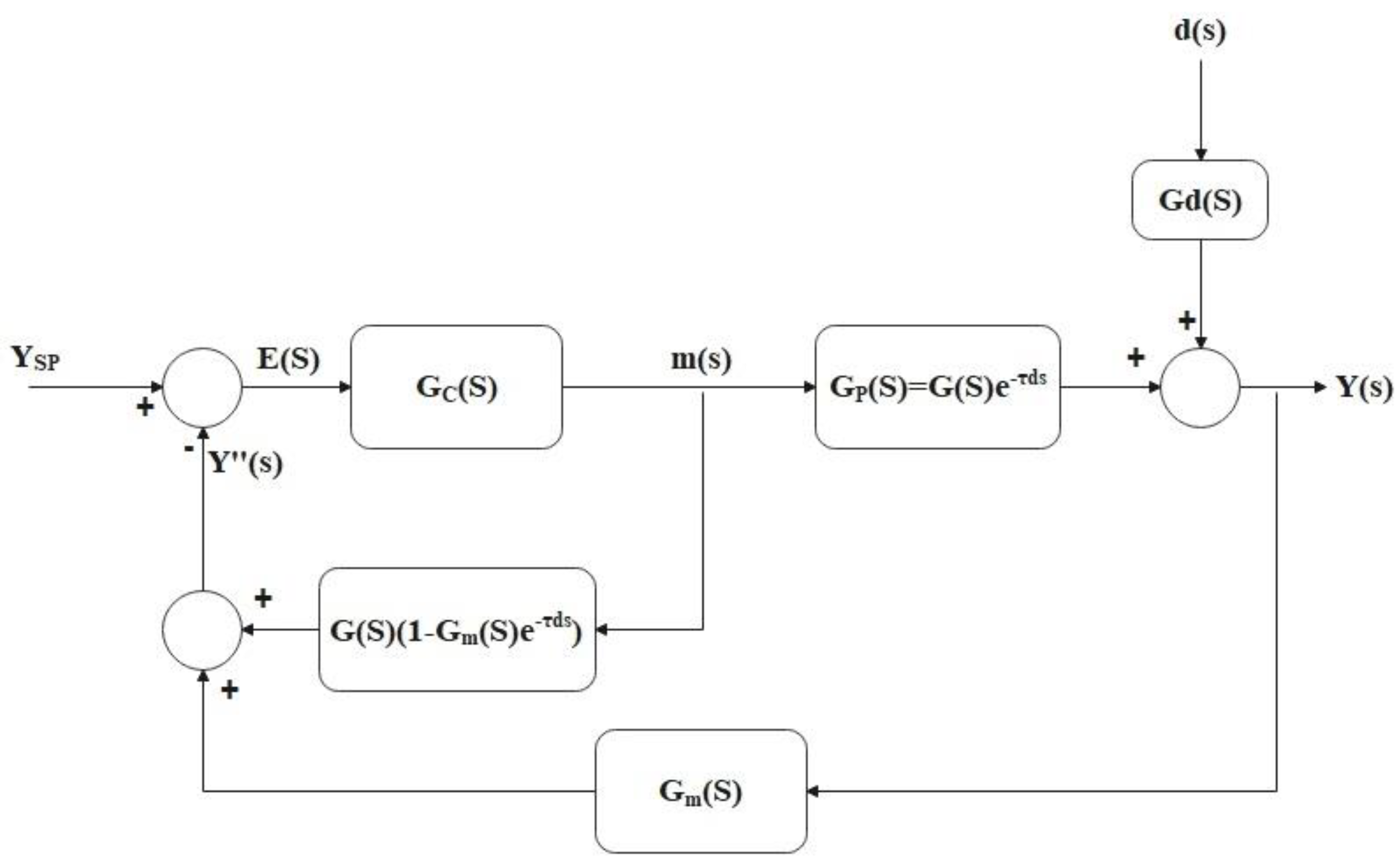
The proposed method in this paper has two phases: one is stabilizing and changes the system behavior from a non-minimum phase to minimum phase, and the other is the precise control of the system (process) by considering system dynamic changes and parametric uncertainty. For the first phase, it is proposed to add the dominant gain transfer function to the open-loop equations of the system (Figure 2).

It is assumed that the measurement transfer function is equal to 1 ($G_m\left(s\right)=1$). The closed-loop transfer functions of this system are in the form of relations (1) and (2).

$$\left(Y_n\left(s\right)\right){\left(Y_{sp,n}\left(s\right)\right)}^{-1}=\left(G_{p,n}\left(s\right)G_{c,n}\left(s\right)\right){\left(1+G_{mb,n}\left(s\right)+G_{c,n}\left(s\right)G_n\left(s\right)\left(1-e^{-{\tau }_{d}s}\right)+G_{p,n}\left(s\right)G_{c,n}\left(s\right)\right)}^{-1}$$

(1)

$$\begin{gathered} \left(Y_n\left(s\right)\right){\left(d_n\left(s\right)\right)}^{-1}=\left(G_{d,n}\left(s\right)+G_{mb,n}\left(s\right)G_{d,n}\left(s\right)+G_{d,n}\left(s\right)G_n\left(s\right)\left(1-e^{-{\tau }_{d}s}\right)G_{c,n}\left(s\right)\right){ \\ \left(1+G_{mb,n}\left(s\right)+G_{c,n}\left(s\right)G_n\left(s\right)\left(1-e^{-{\tau }_{d}s}\right)+G_{c,n}\left(s\right)G_{p,n}\left(s\right)\right)}^{-1} \end{gathered}$$

(2)

In the above relationships, $Y_n\left(S\right),Y_{sp,n}\left(S\right),d_n\left(S\right),G_{mb,n}\left(S\right),G_{p,n}\left(S\right),G_{c,n}S$ and $G_n\left(s\right)$ from left to right, respectively, represent the response matrix, the reference input matrix, the input perturbation matrix, the matrix of predictive functions, the matrix of the process include time delay, matrix functions of the controllers, and finally, the matrix of the process without time delay. In this system, as in the proposed control system in single systems, the input/output of the $G_{mb,n}\left(S\right)$ function, which predicts the nth loop in the control system, must be a function with a minimum phase behavior and a higher gain than other functions in the open-loop function of that loop. The ideal mode for controlling multi-input/output systems is the absence of loop interaction with each other. This happens when the matrix $G_{p,2}\left(s\right)G_{e,2}\left(s\right)$ is a diagonal matrix, in which case, the matrix of the open-loop transfer function of the proposed control system will be as follows:

$$X\left(s\right)=\left[\begin{array}{c}{G}_{mb1}\left(s\right)+G_{p11}\left(s\right)G_{c11}\left(s\right)\\ G_{mb2}\left(s\right)+G_{p22}\left(s\right)G_{c22}\left(s\right)\end{array}\right]$$

(3)

The conditions of the dominant interest concept must be established in a way that the conditions of Equations (4) and (5) in the loops at all frequencies in phase diagrams do not exceed the range from 0 to −180°.

$$\left|G_{mb1}\left(s\right)\right|\ge \left|G_{p11}\left(s\right)G_{c11}\left(s\right)\right|$$

(4)

$$\left|G_{mb2}\left(s\right)\right|\ge \left|G_{p22}\left(s\right)G_{c22}\left(s\right)\right|$$

(5)

This method is effectively expandable for higher-dimensional systems, and it is only necessary to have the necessary conditions to create a dominant interest constraint in the open-loop function of each control loop [29]. If there are interaction effects between the loops, then, for example, in a 2 × 2 open-loop control system, the control system is obtained as follows:

$$Q\left(s\right)=\left(1+G_{mb,11}\left(s\right)+G_{p11}\left(s\right)G_{c11}\left(s\right)\right)\left(1+G_{mb,22}\left(s\right)+G_{p22}\left(s\right)G_{c22}\left(s\right)\right)-G_{p12}\left(s\right)G_{p21}\left(s\right)G_{c11}\left(s\right)G_{c22}\left(s\right)$$

(6)

which, in order to establish the dominant interest constraint, must have the following equation in all or most of the curves so that in the phase diagram of the open-loop function, the control system does not oscillate around the non-minimum phase function diagram and does not exceed 180°:

$$\left|G_{mb,11}\left(s\right)+G_{mb,22}\left(s\right)+G_{mb,11}\left(s\right)G_{mb,22}\left(s\right)\right|\ge \left|\begin{array}{c}{G}_{p22}\left(s\right)G_{c22}\left(s\right)+G_{p11}\left(s\right)G_{c11}\left(s\right)\\ +G_{p11}\left(s\right)G_{p22}\left(s\right)G_{c11}\left(s\right)G_{c22}\left(s\right)\\ +G_{p11}\left(s\right)G_{c11}\left(s\right)G_{mb,22}\left(s\right)\\ +G_{p22}\left(s\right)G_{c22}\left(s\right)G_{mb,11}\left(s\right)\\ -G_{p11}\left(s\right)G_{p21}\left(s\right)G_{c11}\left(s\right)G_{c22}\left(s\right)\end{array}\right|$$

(7)

Of course, a simpler method can be used to apply the proposed method to control systems in which the loops interact. In this method, first, the interactions of the loops are eliminated from various methods, such as controller adjustment methods, and then, the proposed method is used for the assumed system. This method is used in the example given in this article. In the case of selecting the degree of the $G_{mb,j}\left(s\right)$ function given that in multi-input/output systems, the $G_{mb,n}\left(s\right)$ function exists for each loop, we select the same loop separately for the open-loop function; so, selecting the degree of this function is the same as for single-input/output systems, which will be discussed below. In the case of these systems, the general open-loop function can be represented as Equation (8):

$$\begin{gathered} overall open-loop transfer function=G_{\infty ,j}\left(s\right)=G_{mb,j}\left(s\right)+G_{sol,j}\left(s\right) \\ =\frac{K_{mb,j}}{D_{mb,j}^{\left(pb\right)}\left(s\right)}+\frac{K_{sol,j}{N}_{sol,j}^{\left(mo\right)}\left(s\right)}{D_{sol,j}^{\left(pb\right)}\left(s\right)}{e}^{-s{t}_{d,j}},j=1,2,\dots ,n \end{gathered}$$

(8)

In the above relation, $G_{sol,j}\left(s\right)$ is a simple open-loop function in the j-th loop. Additionally, $G_{ool,j}\left(s\right)$ is the general open-loop function for the j-th loop. $K_{mb,j}$ and $K_{sol,j}$ are the compensatory gains and the simple open-loop function, respectively, and $mo$, $pb$, and $po$ are the degrees of the polynomials. Thus, the equation characteristic of the proposed method will be in the form of relation (9).

$$K_{mb,j}{D}_{sol,j}^{\left(po\right)}\left(s\right)+K_{sol,j}{N}_{sol,j}^{\left(mo\right)}\left(s\right)D_{mo,j}^{\left(pb\right)}{e}^{-s{t}_{d}j}=0$$

(9)

In order for the dominant interest condition to be true in the general open-loop function of each loop, Equation (10) must be true.

$$po\ge mo+pb\to pb\le po-mo$$

(10)

Now, if $G_{sol,j}\left(s\right)$ is a suitable function, that is, $po=mo$, for the function to have a minimum phase behavior in relation (10), (i.e., $K_{mb,j}{D}_{sol,j}^{\left(po\right)}\left(s\right)$) must be $pb=0$, whereas if $G_{sol,j}\left(s\right)$ is a strictly suitable function, in order for the function to have a minimum phase behavior in relation (10), it must be $po>mo$; in which case, we have $pb\ge 1$. In this case, $pb=1$ is the most desirable degree because the first-degree functions have a finite phase. Additionally, their phase curves will never reach −180$°$, so they are always stable. In general, the condition for the disappearance of all zeros to the right due to the time delay parameter of the general open-loop function is to establish relation (11):

$$\left|K_{mb,j}{D}_{sol,j}^{\left(po\right)}\left(jw\right)\right|\ge \left|K_{sol,j}{N}_{sol,j}^{\left(mo\right)}\left(jw\right)D_{mb}^{\left(pb\right)}\left(jw\right)e^{-jw{t}_{d,j}}\right|$$

(11)

which is equivalent to relation (12):

$$\left|G_{mb,j}\left(jw\right)\right|\ge \left|G_{sol,j}\left(jw\right)\right|$$

(12)

If there are interference effects between the control loops, then by using Equation (8) and applying a method similar to the one mentioned above, the appropriate degree and gain of the compensating function can be found.

The function G_mb is a first-order transfer function, and it is enough to apply in the conditions of relations (5), (6) and (10). A first-order transfer function only has two parameters: one is the gain and the other is the position of its pole. To set these two parameters, it is enough to meet the mentioned conditions. Of course, various functions can be found that satisfy the mentioned conditions, but definitely only one function can give us the optimal answer. Currently, this optimal transfer function has been obtained by trial and error, but we intend to provide a mechanism to obtain the optimal G_mb in future research.

This function gives us the task of stabilizing the control system and guaranteeing its convergence; the next step is to accurately estimate the amount of delay using a type-2 fuzzy neural network and use it for Smith’s predictive control. Therefore, introducing the existence of such a function is one of the innovations of this article, and the details regarding this function and how to calculate the optimal G_mb will definitely be discussed in future papers.

3.1. Sensitivity Analysis of the Proposed Method

In this section, the robustness of the proposed method to model error is investigated. For simplicity, we discuss the inter-loop control system when there are no interactions. Obviously, this method can be easily generalized to systems with interactions. The characteristic equation of the proposed system is in the form of relation (13) if there are no interactions in the control system.

$$1+G_{mb,n}\left(s\right)+G_{p,n}\left(s\right)G_{c,n}\left(s\right)=0$$

(13)

The error in the model can be represented as $\delta G_{p,n}\left(j\omega \right)=G_{p,n}\left(j\omega \right)-G_{n,n}\left(j\omega \right)$. $\delta G_{p,n}\left(j\omega \right)$ is the difference between the actual model $G_{p,n}\left(j\omega \right)$ and the nominal model $G_{n,n}\left(j\omega \right)$. By placing $\delta G_{p,n}\left(j\omega \right)$ in Equation (14), we will obtain Equation (14).

$$1+G_{mb,n}\left(j\omega \right)+G_{n,n}\left(j\omega \right)G_{c,n}\left(j\omega \right)+\delta G_n\left(j\omega \right)G_{c,n}\left(j\omega \right)=0$$

(14)

Through Equation (15), we can obtain the norm of the highest error range of the model, which will be Equation (15)

$$\left|\delta G_{p,n}\left(j\omega \right)\right|=\frac{\left|1+G_{mb,n}\left(j\omega \right)+G_{n,n}\left(j\omega \right)G_{c,n}\left(j\omega \right)\right|}{\left|G_{c,n}\left(j\omega \right)\right|}$$

(15)

In this way, we can obtain the norm obtained for a typical feedback loop:

$$\left|\delta G_{p,n}\left(j\omega \right)\right|=\frac{\left|1+G_{n,n}\left(j\omega \right)G_{c,n}\left(j\omega \right)\right|}{\left|G_{c,n}\left(j\omega \right)\right|}$$

(16)

According to Equations (15) and (16), under equal conditions, due to the $G_{mb,n}\left(s\right)$ function, the norm of the highest model error range in the proposed method is larger than a normal feedback loop. Therefore, it can be said that the proposed method is more resistant to model error. As a result, it can be said that the proposed method is more flexible in terms of removing model errors.

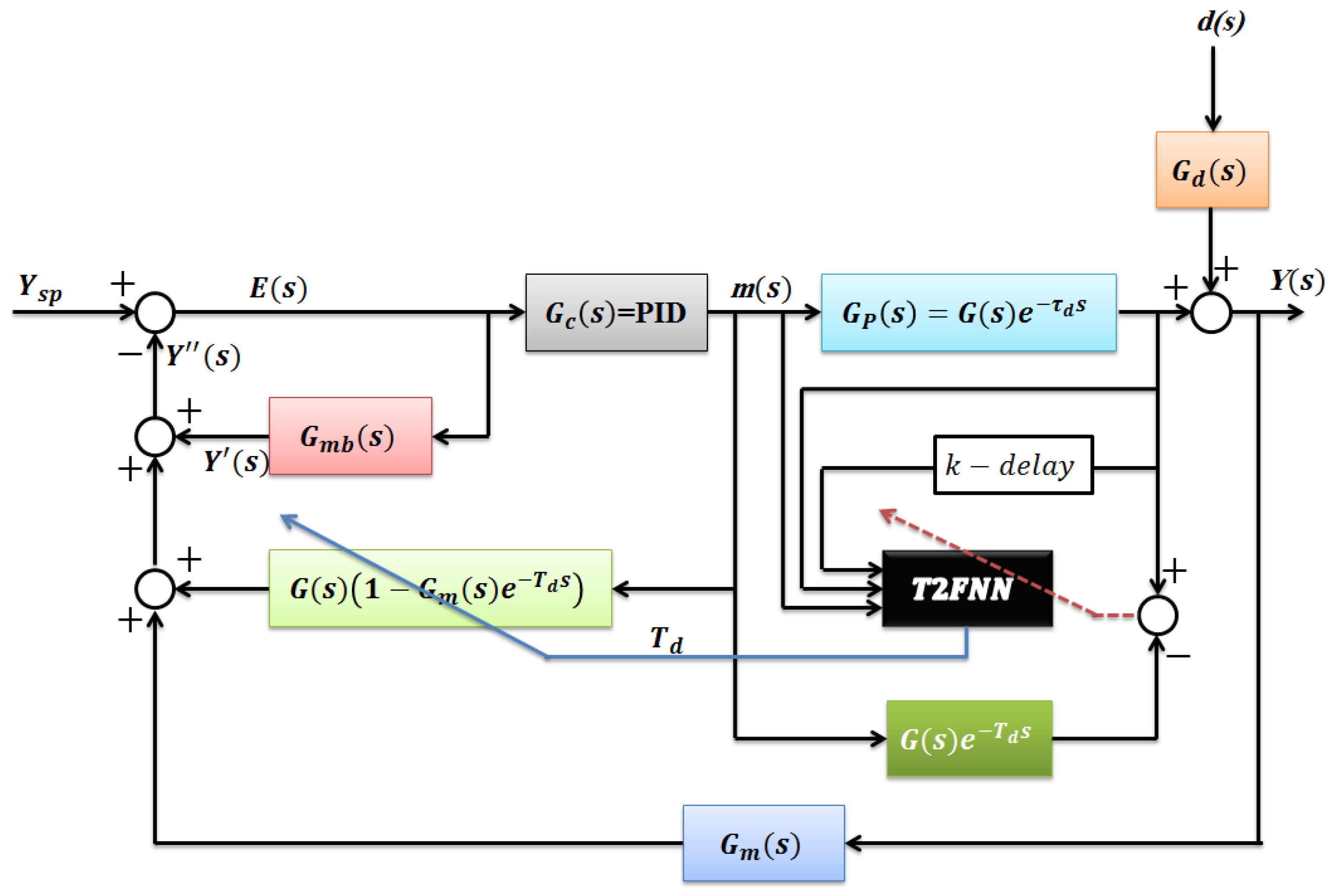
In the second phase, it is time to accurately estimate the amount of system latency. This is effectively completed using a type-2 fuzzy neural network (Figure 3).

Since the analysis is based on the transfer functions and is unlike the state space equations, the input cannot be separated, so the sensitivity analysis is presented only based on the uncertainty of the model. A control system, if it is designed correctly, can consider disturbance as an uncertainty of the model, reduce its effect, and provide the appropriate response. Two important challenges of a control system are uncertainty in the model and the presence of disturbances. Therefore, in order to evaluate the control system, we had to apply both challenges, and fortunately, the proposed method came out victorious.

Figure 3 shows the general structure of the process control system (including both phases). The T2FNN inputs are: the process inputs, process outputs, as well as the process outputs of the previous moments. The output of the type-2 fuzzy neural network is the instantaneous estimation of the time delay of the process. Any change in process dynamics and any factor that changes the system time delay (such as time-lapse and system wear) is immediately observed by the type-2 fuzzy system, and a new ${\mathrm{T}}_{\mathrm{d}}$ is generated.

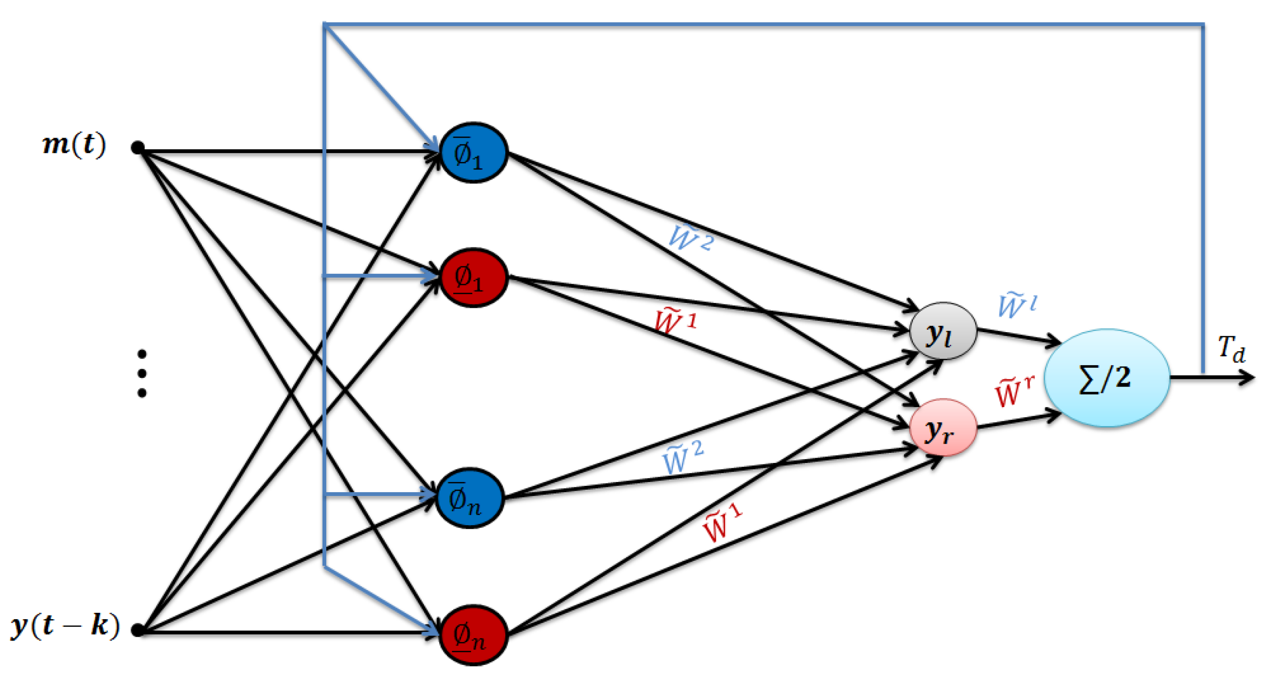
3.2. Type-2 Fuzzy System

In this section, the structure of type-2 fuzzy systems is introduced. Figure 3 shows the proposed type 2 fuzzy system.

The calculations of the first layer are as follows:

$$\{\begin{array}{l}{\overline{\varnothing }}_{ji}\left(x_j\right)=\{\begin{array}{lr}{(x_j-c_{ji}^1)}^2& x_j<c_{ji}^1\\ 1& c_{ji}^1\le x_j\le c_{ji}^2\\ {(x_j-c_{ji}^2)}^2& x_j>c_{ji}^2\end{array}\\ {\underset{¯}{\varnothing }}_{ji}\left(x_j\right)=\{\begin{array}{lr}{(x_j-c_{ji}^2)}^2& x_j\le \frac{c_{ji}^1+c_{ji}^2}{2}\\ {(x_j-c_{ji}^1)}^2& x_j>\frac{c_{ji}^1+c_{ji}^2}{2}\end{array}\end{array}$$

(17)

The upper and lower of the $i\mathrm{th}$ neuron and the $j\mathrm{th}$ input are denoted by ${\overline{\varnothing }}_{ji}$ and ${\underset{\_}{\varnothing }}_{ji}$, respectively. Therefore, the outputs of the first layer are as follows:

$$\{\begin{array}{c}{\overline{\varnothing }}_i\left(x\right)=\exp \left(-\frac{{{\displaystyle \sum }}_{j=1}^{n+1}{\tilde{\varnothing }}_{ji}\left(x_j\right)}{{\sigma }_i^2}\right)\\ {\underset{\_}{\varnothing }}_i\left(x\right)=\exp \left(-\frac{{{\displaystyle \sum }}_{j=1}^{n+1}{\underset{\_}{\varnothing }}_{ji}\left(x_j\right)}{{\sigma }_i^2}\right)\end{array}$$

(18)

where ${\overline{\varnothing }}_i$ and ${\underset{\_}{\varnothing }}_i$ are the upper and lower of the $i\mathrm{th}$ neuron $\left(i=1, 2,\dots ,m\right)$, respectively. $x\in \left(x_j\right), j=1,\dots ,n$ is the input vector, and $c_{ji}\in \left[c_{ji}^1,c_{ji}^2\right]$ is the center of all the type-2 fuzzy neurons. Next, the left and right endpoints of the second layer are as follows:

$$\{\begin{array}{l}{\hat{y}}_l=\frac{{\sum }_{i=1}^q{\overline{\varnothing }}_i(x)c_{w_i}^2{\sigma }_{w_i}+{\sum }_{i=q+1}^m{\underset{¯}{\varnothing }}_i(x)c_{w_i}^1{\sigma }_{w_i}}{{\sum }_{i=1}^q{\overline{\varnothing }}_i(x){\sigma }_{w_i}+{\sum }_{i=q+1}^m{\underset{¯}{\varnothing }}_i(x){\sigma }_{w_i}}\\ {\hat{y}}_r=\frac{{\sum }_{i=1}^p{\underset{¯}{\varnothing }}_i(x)c_{w_i}^1{\sigma }_{w_i}+{\sum }_{i=p+1}^m{\overline{\varnothing }}_i(x)c_{w_i}^2{\sigma }_{w_i}}{{\sum }_{i=1}^p{\underset{¯}{\varnothing }}_i(x){\sigma }_{w_i}+{\sum }_{i=p+1}^m{\overline{\varnothing }}_i(x){\sigma }_{w_i}}\end{array}$$

(19)

where $p$ and $q$ are the left and right switching points the type-2 fuzzy system, which can be calculated using the trial-and-error method or the Karnik–Mendel (KM) algorithm. Additionally, $m$, $w_i$, $c_{w_i}$, and ${\sigma }_{w_i}$ are the mean value of the first-layer neurons, the weights, the center of the weights, and the spread of the weights, respectively. Lastly, the general output of the network can be derived as follows:

$$\hat{y}=\frac{1}{2}\frac{{{\displaystyle \sum }}_{i=1}^q{\hat{y}}_r{c}_{w_i}^r{\sigma }_{w_i}+{{\displaystyle \sum }}_{i=q+1}^m{\hat{y}}_l{c}_{w_i}^l{\sigma }_{w_i}}{{{\displaystyle \sum }}_{i=1}^q{\hat{y}}_r{\sigma }_{w_i}+{{\displaystyle \sum }}_{i=q+1}^m{\hat{y}}_l{\sigma }_{w_i}}$$

(20)

In Equation (20), $c_{w_i}^r$ and $c_{w_i}^l$ are the centers of ${\tilde{W}}^r$ and ${\tilde{W}}^l$, respectively. The gradient descent method is used to teach the network. See [42] for more details.

4. Simulation

In the following, there are two examples of using the proposed system to control multi-input/output processes and how it is used for these systems.

Example 1: The process function of the distillation tower Wood-Berry, which is a well-known function in the field of multi-input/output systems, is considered as follows [30]:

$$G_p\left(s\right)=\left[\begin{array}{cc}\frac{12.8e^{-s}}{16.7s+1}& \frac{-18.9e^{-3s}}{21s+1}\\ \frac{6.6e^{-7s}}{10.9s+1}& \frac{-19.4e^{-3s}}{14.4s+1}\end{array}\right]$$

The first point to consider in solving these problems is the interaction of control loops Is on each other. In order for the loops not to interact with each other, the product of $G_p\times G_c$ must be the product of a diagonal matrix. Various methods are used to diameter the open-loop function matrix of the control system. In some references, this is achieved using decouplers [31,32,33,34,35], and in others, by adjusting the controller parameters [36,37,38,39,40]. This operation is performed. In this example, the second method is used. A method according to which the parameters of the controllers are adjusted so that the loops do not interact with each other is presented in [37]. Based on this method, for this example, the parameters of the controllers for the two control loops are obtained as $G_{c1}=0.547+\frac{0.0915}{s}$ and $G_{c2}=-0.107-\frac{0.021}{s}$ for the PI controllers.

In the proposed method, to design the control structure, we must first select the $G_{mb,n}\left(s\right)$ function. Given that in this example, we want to show the resistance of the proposed method to the model error for all time delay parameters in $G_{pij}\left(s\right)$, the probability of error is set as up to +50%. We consider the percentage in the proposed method, the $G_{mb,n}\left(s\right)$ function must be selected so that it has the ability to cover the highest error limit so that at most frequencies, the dominant interest condition is observed, and the open-loop function has a minimum phase behavior. By selecting $G_{mb1}\left(s\right)=\frac{1}{s+1}$ for the first loop and $G_{mb2}\left(s\right)=\frac{0.5}{s+1}$ for the second loop, as shown in Figure 3 and Figure 4, the dominant interest condition for the highest model error range norm, with the conditions mentioned, is met. Figure 5 and Figure 6 show the frequency response diagram for the open-loop function of the first and second loops in the proposed control structure.

As can be seen in these figures, the condition for the superiority of the $G_{mb,n}\left(s\right)$ gain in most frequencies is such that the phase diagram is limited before reaching the −180° point in these two loops. Therefore, it can be concluded that the selection of $G_{mb,ii}\left(s\right)$ is appropriate in both loops. Additionally, the minimum phase behavior of the open-loop function in the proposed method is one of the advantages of this method compared to the methods in which the open-loop function of the control system has non-minimum phase behavior. Figure 7, Figure 8, Figure 9 and Figure 10 show the performance of Smith’s predictive control systems, Smith’s predictor with dominant gain, and the proposed control system (Smith’s predictor with dominant gain and type-2 fuzzy estimator for time delay). In this example, $y_1$ is distillate composition, $y_2$ is bottom composition, and $u$ is reflux flow rate. 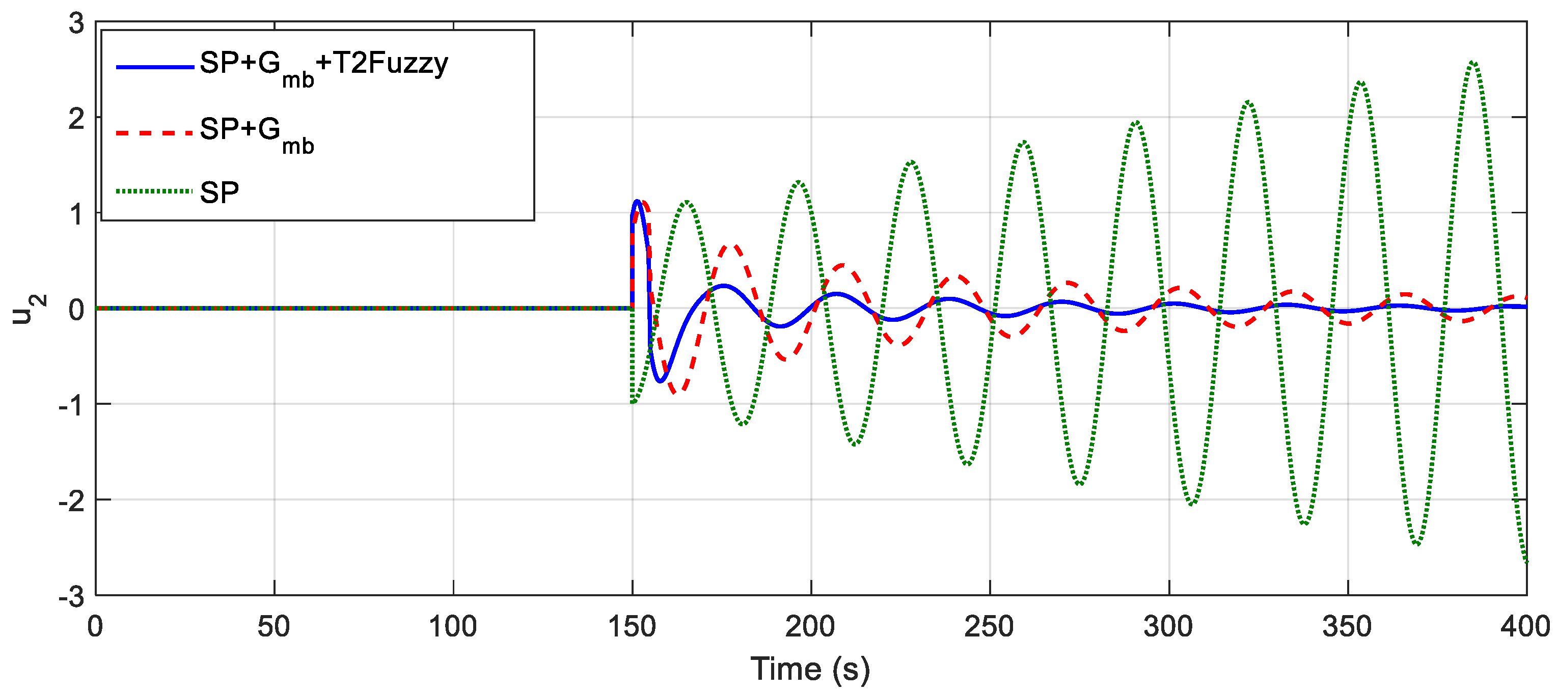It should be noted that the reference for $y_1$ is the step signal with the step time t = 50 s, and for $y_2$, this is the step with the step time t = 200 s. The control signals $u_1$ and $u_2$ are shown in Figure 8 and Figure 9, respectively.

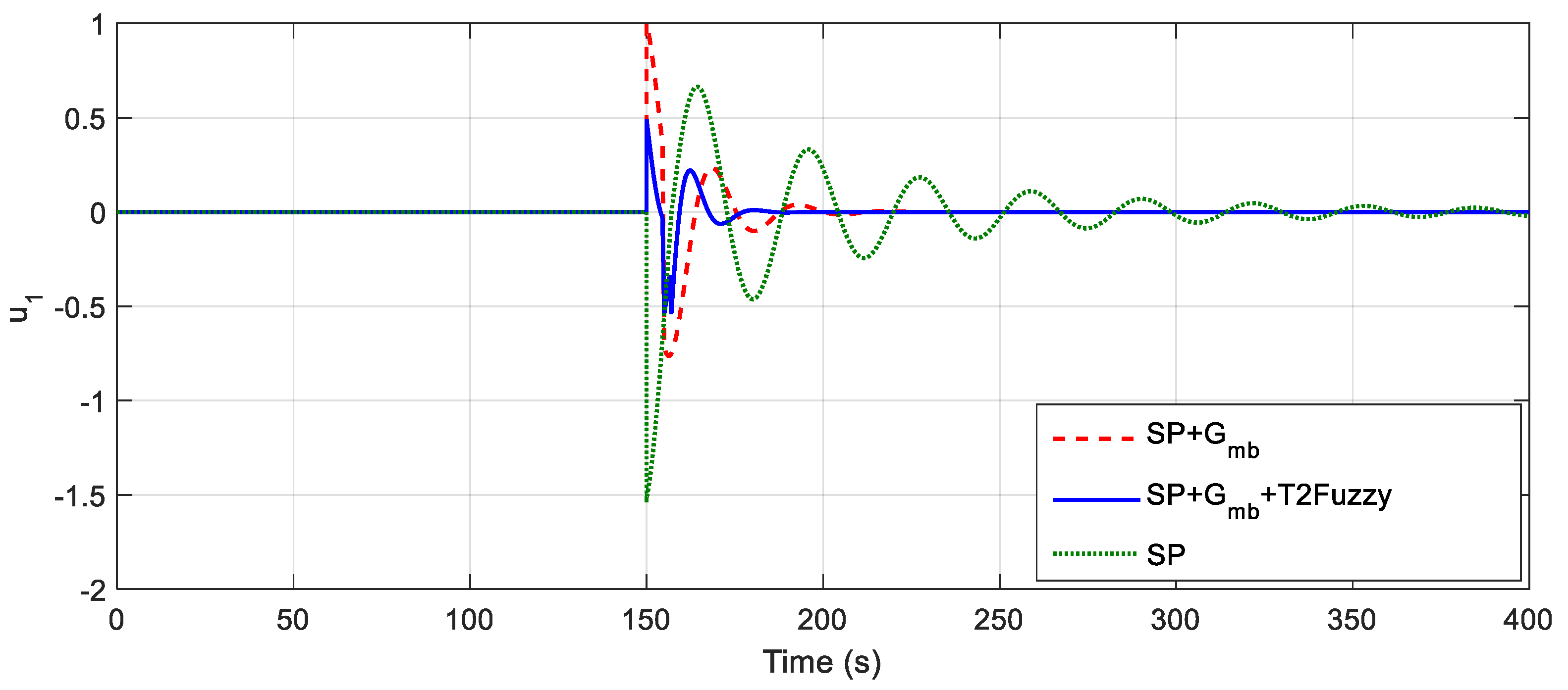
It is clear from Figure 7, Figure 8, Figure 9 and Figure 10 that the proposed method (Smith’s predictor with dominant gain and type-2 fuzzy estimator) performs better both in terms of accuracy and response speed. In addition, the proposed method has a minimum control cost. In order to challenge the control systems, a disturbance signal (a pulse with a height of 1 and a width of 2 s) is applied at the moment t = 150 s (Figure 11, Figure 12, Figure 13 and Figure 14).

It can be seen from Figure 11, Figure 12, Figure 13 and Figure 14 that the performance of the proposed method with a type-2 fuzzy estimator is very good, and the system reaches its equilibrium point in less than 20 s. In the meantime, the worst performance is related to Smith’s pure predictive method, which fluctuates more than 200 s after applying disturbance.

Another challenge for the control system is the uncertainty or changes in the parameters of the controlled system (process). This challenge inevitably arises because systems wear out over time and their behavior changes. Next, it is assumed that the system parameters (numerator and denominators coefficients of the transfer function as well as time delay) are doubled at t = 150 s (Figure 15, Figure 16, Figure 17 and Figure 18).

Interesting results can be seen in Figure 11, Figure 12, Figure 13, Figure 14, Figure 15, Figure 16, Figure 17 and Figure 18. Smith’s pure prediction method diverges against large changes in parameters. Since after the initial adjustment of Smith’s prediction method, it is assumed that the system does not change behavior (or at least changes very little), this method has nothing to say in the face of major changes. On the other hand, it is observed that the convergence of the control system is adjusted by adding the dominant gain transfer function ($G_{mb}$) to Smith’s predictive method. Finally, with the addition of a type-2 fuzzy estimator to the control system, the accuracy and speed of convergence is dramatically improved. It should be noted that for example 1, the phase margin is ${43}^{°}$ and the gain margin is 18.6 dB.

Example 2: A $3\times 3$ subsystem of the shell heavy-oil fractionator is as follows [31]:

$$G\left(s\right)=\left[\begin{array}{ccc}\frac{4.05e^{-27s}}{50s+1}& \frac{1.77e^{-28s}}{60s+1}& \frac{5.88e^{-27s}}{50s+1}\\ \frac{5.39e^{-18s}}{50s+1}& \frac{5.27e^{-8s}}{60s+1}& \frac{6.9e^{-15s}}{60s+1}\\ \frac{4.38e^{-20s}}{33s+1}& \frac{4.42e^{-22s}}{44s+1}& \frac{7.2}{19s+1}\end{array}\right]$$

In order to avoid cluttering the article and confusing the readers, we do not intend to carry out all the steps in Example 1 for this example, but only to show the ability of the control system for the system with any number of inputs and outputs and any amount of interaction. Based on this method, for this example, the parameters of the controllers for the three control loops are obtained as $G_{c1}=0.662+\frac{0.0365}{s}$, $G_{c2}=1+\frac{0.019}{s}$ and $G_{c3}=4+\frac{0.077}{s}$. 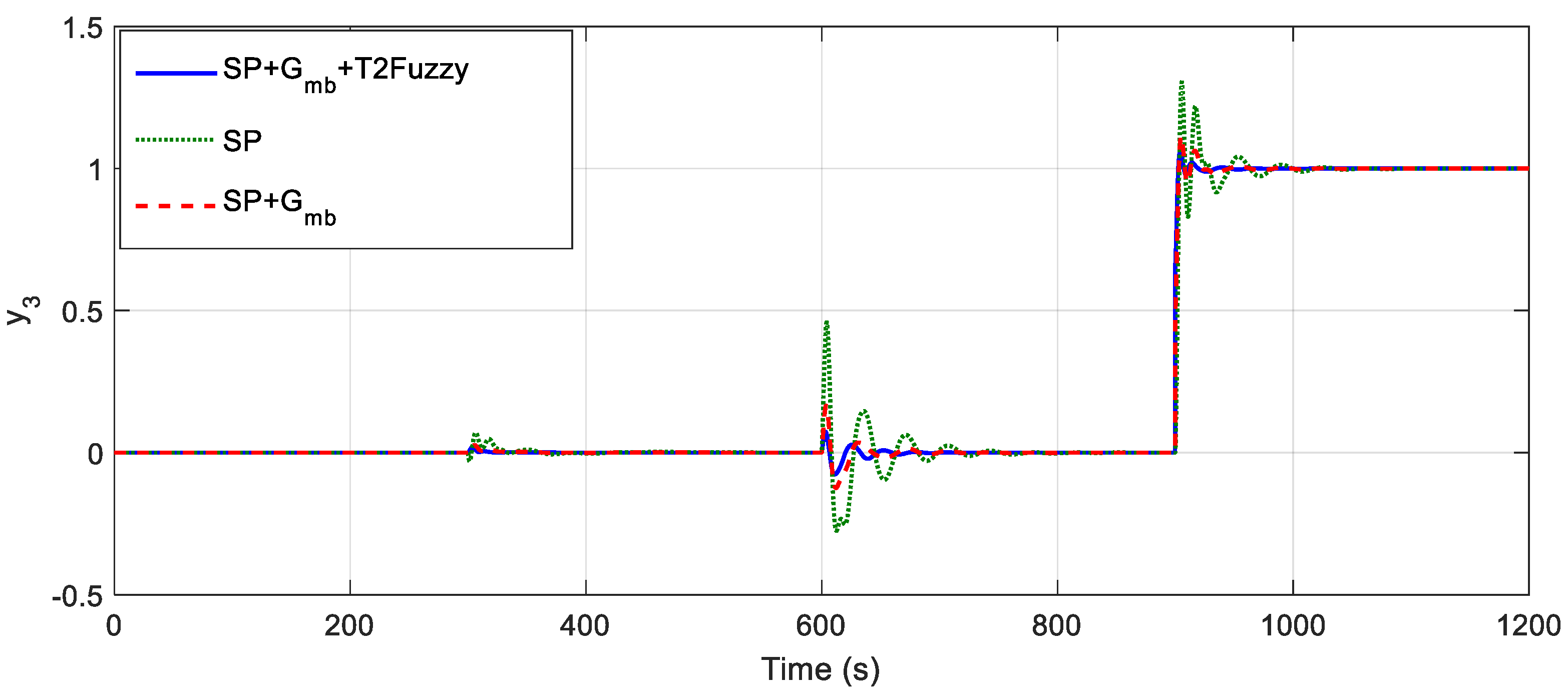Figure 19, Figure 20 and Figure 21 show the performance of Smith’s predictive control systems, Smith’s predictor with dominant gain, and the proposed control system (Smith’s predictor with dominant gain and a type-2 fuzzy estimator for time delay). It should be noted that the reference for $y_1$ is the step signal with the step time t = 300 s; for $y_2$, this is the step with the step time t = 600 s; and for $y_3$, this is the step with the step time t = 900. The control signals $u_1$, $u_2$, and $u_3$ are shown in Figure 22, Figure 23 and Figure 24, respectively. In this example, $y_1$ is the top endpoint composition, $y_2$ is the side end point composition, and $y_3$ is the bottom reflux temperature. The inputs are the top drawn flow rate ($u_1)$, the side drawn flow rate ($u_2)$, and the bottom reflux heat duty ($u_3)$. It should be noted that the reference for $y_1$ is the step signal with the step time t = 300 s; for $y_2$, this is the step with the step time t = 600 s; and for $y_3$, this is the step with the step time t = 900.

Example 2 is a system with high latency and relatively strong interaction. It can be seen from Figure 18, Figure 19 and Figure 20 that the proposed method has been able to successfully provide a suitable answer. It is carefully observed in Figure 18 that by applying the second step, the Smith’s pure predictive method has more than 150% overshoot, Smith’s predictive method with dominant gain has 60%, and finally, this method with a type-2 fuzzy estimator has less 40%. The minimum cost of the control signal of the proposed method is clearly shown in Figure 22.

Table 1. A comparison between some methods for example 2.

	${\mathit{y}}_{\mathbf{1}}$	${\mathit{y}}_{\mathbf{2}}$	${\mathit{y}}_{\mathbf{3}}$
SP	0.135	0.089	0.051
$\mathrm{SP}+G_{mb}$	0.073	0.059	0.038
$\mathrm{SP}+G_{mb}$ + T2Fuzzy	0.061	0.045	0.032
Method of [43]	0.063	0.055	0.040
Method of [44]	0.061	0.049	0.034

shows a comparison between some methods based on root mean square error (RMSE) criterion. It should be noted that for example 2, the phase margin is ${29}^{°}$ and the gain margin is 12.2 dB.

It can be seen from Table 1 that the proposed method has the best answer in terms of accuracy (RMSE criterion). Although in control $y_1$, the method of [41] has an RMSE equal to our method, for the other two outputs, our proposed method works better.

5. Conclusions

In this paper, a new method based on Smith’s predictor for controlling time-delayed MIMO systems is presented. The proposed control system had two phases: one is the addition of a transfer function with a dominant gain to stabilize the system, and the second phase is the use of a type-2 fuzzy estimator to estimate the system time delay online. In the simulation with two examples, it was shown that the proposed method is very robust and can control the system (process) well with proper accuracy and speed of response. Control challenges, disturbance and parametric uncertainty were also applied, which showed that the proposed system is highly efficient in facing these two challenges. The simulation results clearly showed how much the addition of the transfer function with the dominant gain can improve the performance of the control system. In addition, a type-2 fuzzy system with the ability to accurately estimate the amount of time delay was able to provide a very suitable answer. As a suggestion to continue the work, in addition to estimating the amount of time delay, the process parameters can also be estimated using the fuzzy system. In addition, other more accurate estimators (type-3 fuzzy, etc.) can be used.