On the Dynamics of New 4D and 6D Hyperchaotic Systems

Abstract

One of the most interesting problems is the investigation of the boundaries of chaotic or hyperchaotic systems. In addition to estimating the Lyapunov and Hausdorff dimensions, it can be applied in chaos control and chaos synchronization. In this paper, by means of the analytical optimization, comparison principle, and generalized Lyapunov function theory, we find the ultimate bound set for a new six-dimensional hyperchaotic system and the globally exponentially attractive set for a new four-dimensional Lorenz- type hyperchaotic system. The novelty of this paper is that it not only shows the 4D hyperchaotic system is globally confined but also presents a collection of global trapping regions of this system. Furthermore, it demonstrates that the trajectories of the 4D hyperchaotic system move at an exponential rate from outside the trapping zone to its inside. Finally, some numerical simulations are shown to demonstrate the efficacy of the findings.

1. Introduction

In 1979, Rössler made the first mention of hyperchaos [1]. Numerous hyperchaotic systems have since been introduced in nonlinear research. A hyperchaotic system differs from a chaotic system in that it has two or more positive Lyapunov exponents, which explains why it has a more intricate algebraic structure. Moreover, due to its several engineering applications in technological fields such as secure communications [2], nonlinear circuits [3], lasers [4], neural network [5], artificial intelligence [6], control [7], synchronization [8], and so on, many scientists have concentrated on studying the various dynamical behaviors of new hyperchaotic systems including bifurcations, control problems, and bounds estimation.

In particular, the ultimate boundedness is an effective instrument for the investigation of a new chaotic system’s qualitative behavior. If we are able to demonstrate that a chaotic or hyperchaotic system has a globally trapping region, we can deduce that the system does not have equilibrium points, periodic or quasi-periodic solutions, or any other chaotic, hyperchaotic, or hidden attractors outside the trapping region. As a result, the analysis of the system’s dynamics is substantially facilitated and simplified [9]. Additionally, the estimation of a chaotic system’s bounds is crucial for studying chaos synchronization, chaos control, and determining Hausdorff and Lyapunov dimensions [10,11,12,13,14,15].

In 1987, Leonov et al. examined the boundedness of the famous Lorenz system [16,17]. Since then, several works have studied the ultimate boundedness of other new $3D$ chaotic systems [18,19,20] and new hyperchaotic systems [21,22,23]. However, as there are no established procedures for producing the Lyapunov functions, particularly for high dimensional systems, it is frequently challenging to find this estimate.

Motivated by the aforementioned discussion, using the analytical optimization, comparison principle, and generalized Lyapunov function theory, we found the ultimate bound set for a new six-dimensional hyperchaotic system and the globally exponentially attractive set for a new four-dimensional Lorenz-type hyperchaotic system. In particular, we came to the conclusion that the trajectories of the new 4D hyperchaotic system advance exponentially from outside the trapping zone to its inner. Finally, to illustrate the main results, some numerical simulations are provided.

2. Mathematical Models

In 2018, Lingzhi Yi et al. constructed a new six-dimensional hyperchaotic system [24]:

$$\left\{\begin{array}{c}{x}^{{}^{\prime }}=ay-ax+w\\ y^{\prime }=cx-y-xz-v\\ z^{\prime }=-bz+xy\\ w^{\prime }=dw-yz\\ v^{\prime }=ry\\ u^{\prime }=-eu+zw\end{array}\right.$$

(1)

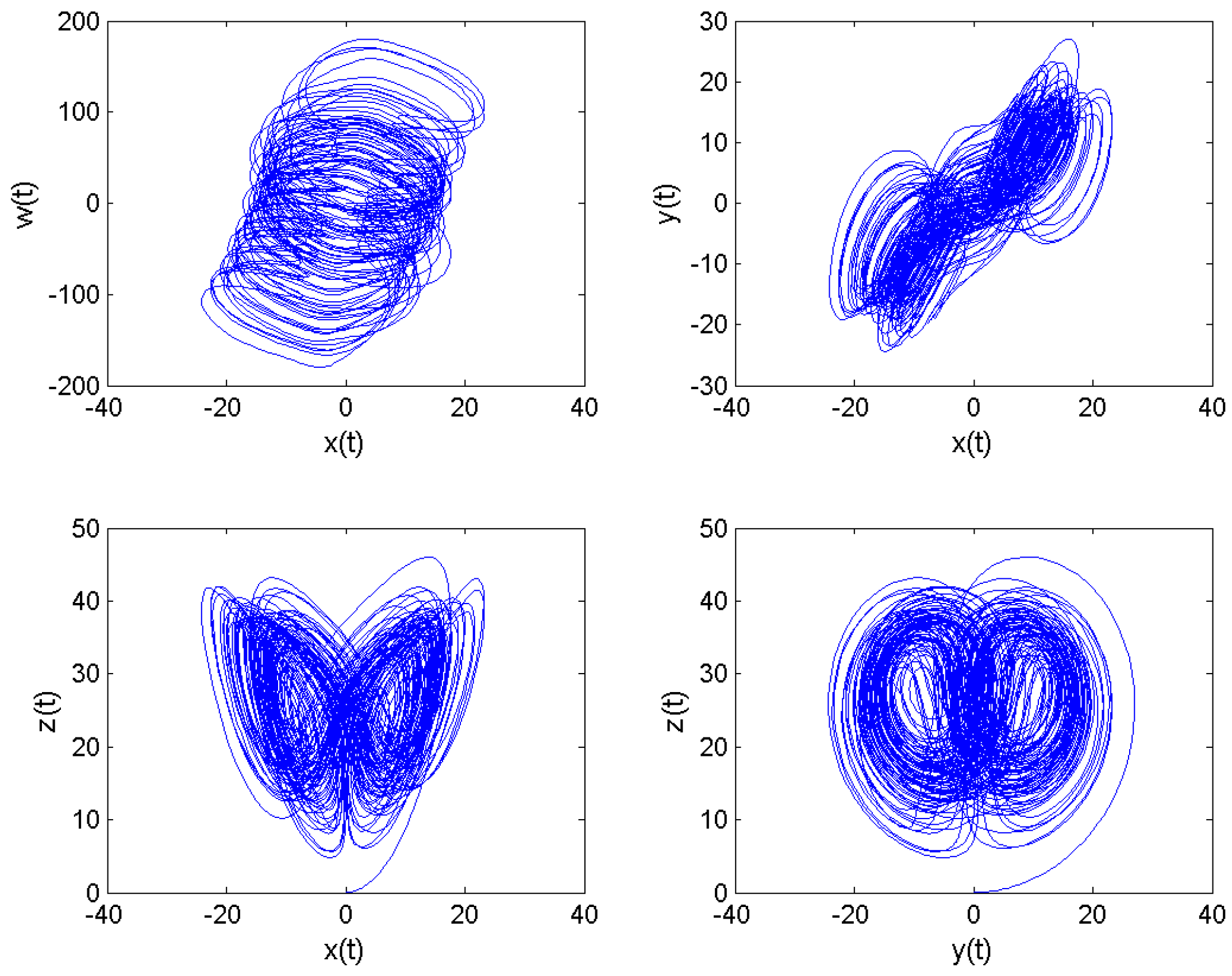
where a, b, c, d, e, r are real parameters with $a>0$, $b>0$, $c>0$, $e>0$, $r>0$ and $d<0.$ When $\left(a,b,c,d,e,r\right)=\left(10,{\displaystyle \frac{8}{3}},28,-1,10,3\right)$, the Lyapunov exponents are ${\lambda }_{L{E}_1}=0.362485$, ${\lambda }_{L{E}_2}=0.24709$, ${\lambda }_{L{E}_3}=0$, ${\lambda }_{L{E}_4}=-0.225698$, ${\lambda }_{L{E}_5}=-10.0017$, ${\lambda }_{L{E}_6}=-$$15.0708$ (see [24]) and consequently, system $\left(1\right)$ displays a typical hyperchaotic attratctor. The corresponding two-dimensional phase diagrams in $\left(x,y\right)$, $\left(x,z\right)$, $\left(y,z\right)$, $\left(x,w\right)$ spaces are shown in Figure 1.

In [24], some basic dynamical characteristics including bifurcation diagrams, Lyapunov exponents and phase portraits of the new 6-D hyperchaotic system $\left(1\right)$ have been investigated, but no explicit ultimate bound set has been obtained for this high dimensional chaotic system. In this paper we will explore this subject.

On the other hand, a new 4-D Lorenz-type system is constructed in [25], which is described as

$$\left\{\begin{array}{c}{x}^{{}^{\prime }}=ay-ax\\ y^{\prime }=bx-cy-xz+w\\ z^{\prime }=xy-dz\\ w^{\prime }=-rw-ky\end{array}\right.$$

(2)

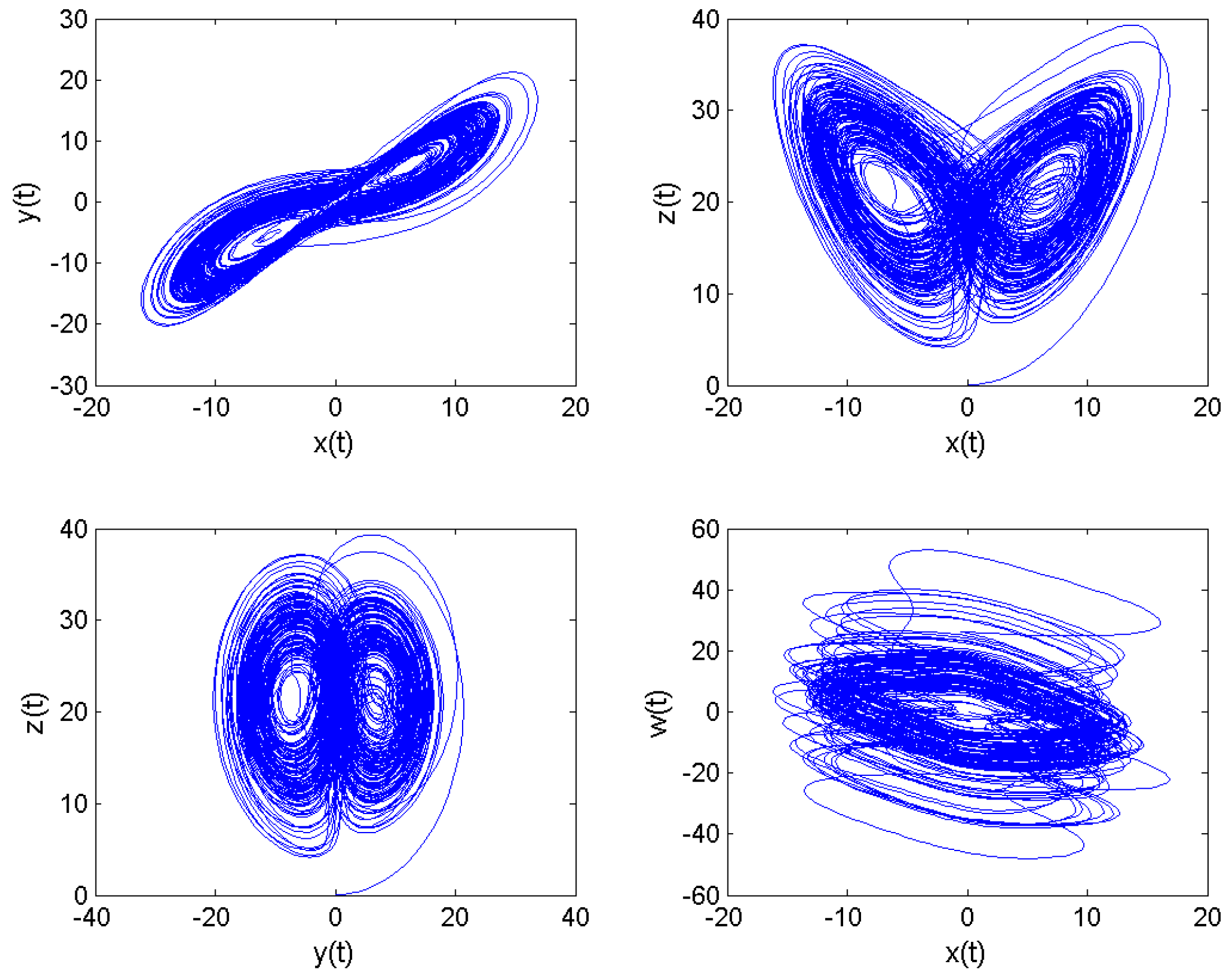
where a, b, c, d are positive real parameters. When $\left(a,b,c,d,k,r\right)=\left(12,23,1,2.1,6,0.2\right)$, the Lyapunov exponents are ${\lambda }_{L{E}_1}=0.1740$, ${\lambda }_{L{E}_2}=0.1314$, ${\lambda }_{L{E}_3}=0$, ${\lambda }_{L{E}_4}=-15.6059$ (see [25]). The two positive Lyapunov exponents indicate that system $\left(2\right)$ is hyperchaotic and the projections of the attractor are shown in Figure 2.

Although [25] gives the ultimate bound and positively invariant set of system $\left(2\right)$, it does not give the estimation of the trajectories rate. In this paper, we will present a collection of globally exponentially attractive sets to specify the pace at which trajectories go from the outside of the trapping region to its inside.

3. Ultimate Bound Set for the New 6D Hyperchaotic System

In this part, we will studied the boundedness of the new 6D hyperchaotic system $\left(1\right)$ for any $a>0$, $b>0$, $c>0$, $e>0$, $r>0$ and $d<0$.

Theorem 1.

When $a>0$, $b>0$, $c>0$, $e>0$, $r>0$ and $d<0$, the following set

$${\Omega }_1=\left\{\begin{array}{c}\left(x,y,z,w,v,u\right)/x^2\le {\displaystyle \frac{{\left(\left(c-da\right)L\sqrt{r}+L^2\right)}^2}{d^2{r}^2{a}^2}},r{y}^2+r{\left(z-c\right)}^2+v^2\le L^2,\\ w^2\le {{\displaystyle \frac{\left(L^2+cL\sqrt{r}\right)}{r^2{d}^2}}}^2,u^2\le {\displaystyle \frac{{\left(L+c\sqrt{r}\right)}^2{\left(L^2+cL\sqrt{r}\right)}^2}{d^2{e}^2{r}^3}}\end{array}\right\}$$

(3)

is the ultimate bound for system $\left(1\right)$, where

$$L^2=\left\{\begin{array}{c}{\displaystyle \frac{r{b}^2{c}^2}{4\left(b-1\right)}},\mathrm{if}b\ge 2\\ r{c}^2,\mathrm{if}b<2\end{array}\right.$$

(4)

Proof of Theorem 1.

Construct the following Lyapunov function

$$V_1=r{y}^2+r{\left(z-c\right)}^2+v^2$$

(5)

Differentiating $V_1$ along the trajectory of system $\left(1\right)$, we can obtain

$$\begin{array}{cc}\hfill \stackrel{.}{V_1}& =2ry{y}^{\prime }+2r\left(z-c\right)z^{\prime }+2v{v}^{\prime }\hfill \\ \hfill & =2ry\left(cx-y-xz-v\right)+2r\left(z-c\right)\left(-bz+xy\right)+2v\left(ry\right)\hfill \\ \hfill & =-2r{y}^2-2rb{z}^2+2rcbz\hfill \\ \hfill & =-2r{y}^2-2rb{\left(z-\frac{c}{2}\right)}^2+\frac{rb{c}^2}{2}\hfill \end{array}$$

(6)

Obviously, $V_1$ is positive definite for $a>0$, $b>0$, $c>0$, $e>0$, $r>0$ and $d<0$. Let $\stackrel{.}{V_1}=0$, then the the surface ${\Gamma }_1$ defined by

$${\Gamma }_1=\left\{\left(y,z\right)/2r{y}^2+2rb{\left(z-\frac{c}{2}\right)}^2=\frac{rb{c}^2}{2},b>0,c>0,r>0\right\}.$$

(7)

is an ellipsoid in ${\mathbb{R}}^2.$ Outside ${\Gamma }_1$, we have $\stackrel{.}{V_1}<0$, while inside ${\Gamma }_1$, we have $\stackrel{.}{V_1}>0$. Since $V_1=r{y}^2+r{\left(z-c\right)}^2+{\nu }^2$ is a continuous function and ${\Gamma }_1$ is a bounded closed set, then the function $V_1$ can reach its maximum value $L^2=max{V}_{1\left(y,z\right)\in {\Gamma }_1}.$ In order to calculate it, we have to solve the following optimization problem

$$\left\{\begin{array}{c}max{V}_1=max\left\{r{y}^2+r{\left(z-c\right)}^2+v^2\right\}\\ s.t.2r{y}^2+2rb{\left(z-{\displaystyle \frac{c}{2}}\right)}^2={\displaystyle \frac{rb{c}^2}{2}}\end{array}\right.$$

(8)

Which is equivalent to

$$\left\{\begin{array}{c}max{V}_1=max\left\{r{y}^2+r{\left(z-c\right)}^2+v^2\right\}\\ s.t.{\displaystyle \frac{y^2}{{\displaystyle \frac{b{c}^2}{4}}}}+{\displaystyle \frac{{\left(z-{\displaystyle \frac{c}{2}}\right)}^2}{{\displaystyle \frac{c^2}{4}}}}=1\end{array}\right.$$

(9)

By the Lagrange multiplier method, define

$$G=r{y}^2+r{\left(z-c\right)}^2+{\nu }^2+\lambda \left[r{y}^2+rb{\left(z-\frac{c}{2}\right)}^2-\frac{rb{c}^2}{4}\right]$$

(10)

and let

$$\left\{\begin{array}{c}{\displaystyle \frac{\partial G\left(y,z,v\right)}{\partial y}}=2ry+2\lambda ry=0\\ {\displaystyle \frac{\partial G\left(y,z,v\right)}{\partial z}}=2r\left(z-c\right)+2\lambda rb\left(z-{\displaystyle \frac{c}{2}}\right)=0\\ {\displaystyle \frac{\partial G\left(y,z,v\right)}{\partial \nu }}=2v=0\\ {\displaystyle \frac{\partial G\left(y,z,v\right)}{\partial \lambda }}=r{y}^2+rb{\left(z-\frac{c}{2}\right)}^2-{\displaystyle \frac{rb{c}^2}{4}}=0\end{array}\right..$$

(11)

Thus,

• $\left(i\right)$ When $\lambda \ne -1$, we can obtain
• $\left(y,z,v\right)=\left(0,0,0\right)$ and $L^2=max{V}_{1\left(y,z\right)\in {\Gamma }_1}=r{c}^2$
• or
• $\left(y,z,v\right)=\left(0,c,0\right)$ and $L^2=0.$
• $\left(ii\right)$ When $\lambda =-1$, and $b\ge 2$, we can obtain
• $\left(y,z,v\right)=\left(\pm {\displaystyle \frac{bc\sqrt{b-2}}{2\left(1-b\right)}},{\displaystyle \frac{c\left(2-b\right)}{2\left(1-b\right)}},0\right)$ and $L^2={\displaystyle \frac{r{b}^2{c}^2}{4\left(b-1\right)}}$.

Consequently, we conclude that

$$V_1\le \underset{X\in {\Gamma }_1}{max}{V}_1\left(X\right)=L^2=\left\{\begin{array}{c}{\displaystyle \frac{r{b}^2{c}^2}{4\left(b-1\right)}},\mathrm{if}b\ge 2\\ r{c}^2,\mathrm{if}b<2\end{array}\right.$$

(12)

From $\left(12\right)$, we obtain

$$\left|y\right|\le \frac{L}{\sqrt{r}},\left|z\right|\le \frac{L}{\sqrt{r}}+c.$$

(13)

Thus, we have

$$w^{\prime }=dw-yz\le dw+\left|y\right|\left|z\right|\le dw+\frac{L}{\sqrt{r}}\left(\frac{L}{\sqrt{r}}+c\right)$$

(14)

By the comparison principle, we can obtain

$$w\left(t\right)\le \frac{L^2+cL\sqrt{r}}{-dr}+\left(w\left(t_0\right)+\frac{L^2+cL\sqrt{r}}{-dr}\right)e^{d\left(t-t_0\right)},\mathrm{where}d<0$$

(15)

Passing to the limit, we obtain

$$\underset{t\to +\infty }{lim}w\left(t\right)\le \frac{L^2+cL\sqrt{r}}{-dr}.$$

(16)

In other words,

$$w^2\le {{\displaystyle \frac{\left(L^2+cL\sqrt{r}\right)}{r^2{d}^2}}}^2,\mathrm{when}t\to +\infty .$$

(17)

Likewise, we have

$$x^{{}^{\prime }}=-ax+ay+w\le -ax+a\left|y\right|+\left|w\right|\le -ax+\frac{aL}{\sqrt{r}}+\frac{L^2+cL\sqrt{r}}{-dr}$$

(18)

By the comparison principle, we obtain

$$x\left(t\right)\le \frac{\left(c-da\right)L\sqrt{r}+L^2}{-dra}+\left(x\left(t_0\right)+\frac{\left(c-da\right)L\sqrt{r}+L^2}{-dra}\right)e^{-a\left(t-t_0\right)},\mathrm{where}d<0$$

(19)

Thus, we have

$$\underset{t\to +\infty }{lim}x\left(t\right)\le \frac{\left(c-da\right)L\sqrt{r}+L^2}{-dra}.$$

(20)

Furthermore, this gives,

$$x^2\le {{\displaystyle \frac{\left(\left(c-da\right)L\sqrt{r}+L^2\right)}{d^2{r}^2{a}^2}}}^2,\mathrm{when}t\to +\infty .$$

(21)

Furthermore, according to the sixth equation of system $\left(1\right)$, we have

$$u^{\prime }=-eu+zw\le -eu+\left|z\right|\left|w\right|\le -eu+\left(\frac{L+c\sqrt{r}}{\sqrt{r}}\right)\left(\frac{L^2+cL\sqrt{r}}{-dr}\right)$$

(22)

By the comparison principle, we obtain

$$u\left(t\right)\le \frac{\left(L+c\sqrt{r}\right)\left(L^2+cL\sqrt{r}\right)}{-d{r}^{\frac{3}{2}}e}+\left(u\left(t_0\right)+\frac{\left(L+c\sqrt{r}\right)\left(L^2+cL\sqrt{r}\right)}{-d{r}^{\frac{3}{2}}e}\right)e^{-e\left(t-t_0\right)}$$

(23)

So, we obtain

$$\underset{t\to +\infty }{lim}u\left(t\right)\le \frac{\left(L+c\sqrt{r}\right)\left(L^2+cL\sqrt{r}\right)}{-d{r}^{\frac{3}{2}}e}.$$

(24)

That is to say,

$$u^2\le {\displaystyle \frac{{\left(L+c\sqrt{r}\right)}^2{\left(L^2+cL\sqrt{r}\right)}^2}{d^2{e}^2{r}^3}},\mathrm{when}t\to +\infty .$$

(25)

From the above, we deduce that

$${\Omega }_1=\left\{\begin{array}{c}\left(x,y,z,w,v,u\right)/,x^2\le {{\displaystyle \frac{\left(\left(c-da\right)L\sqrt{r}+L^2\right)}{d^2{r}^2{a}^2}}}^2,r{y}^2+r{\left(z-c\right)}^2+v^2\le L^2,\\ w^2\le {{\displaystyle \frac{\left(L^2+cL\sqrt{r}\right)}{r^2{d}^2}}}^2,u^2\le {\displaystyle \frac{{\left(L+c\sqrt{r}\right)}^2{\left(L^2+cL\sqrt{r}\right)}^2}{d^2{e}^2{r}^3}}\end{array}\right\}$$

is the ultimate bound set for the new 6D hyperchaotic system $\left(1\right)$. This completes the proof. □

Numerical Simulations

i. According to Theorem 1, when $a=10$, $b={\displaystyle \frac{8}{3}}$, $c=28$, $d=-1$, $e=10$, $r=3$, we can find that

$$\Phi =\left\{\left(y,z,v\right)/3y^2+3{\left(z-28\right)}^2+v^2\le \frac{{112}^2}{5}\right\}$$

(26)

is the bound set of the 6D hyperchaotic system $\left(1\right)$ in the $\left(y\left(t\right),z\left(t\right),v\left(t\right)\right)$ space.

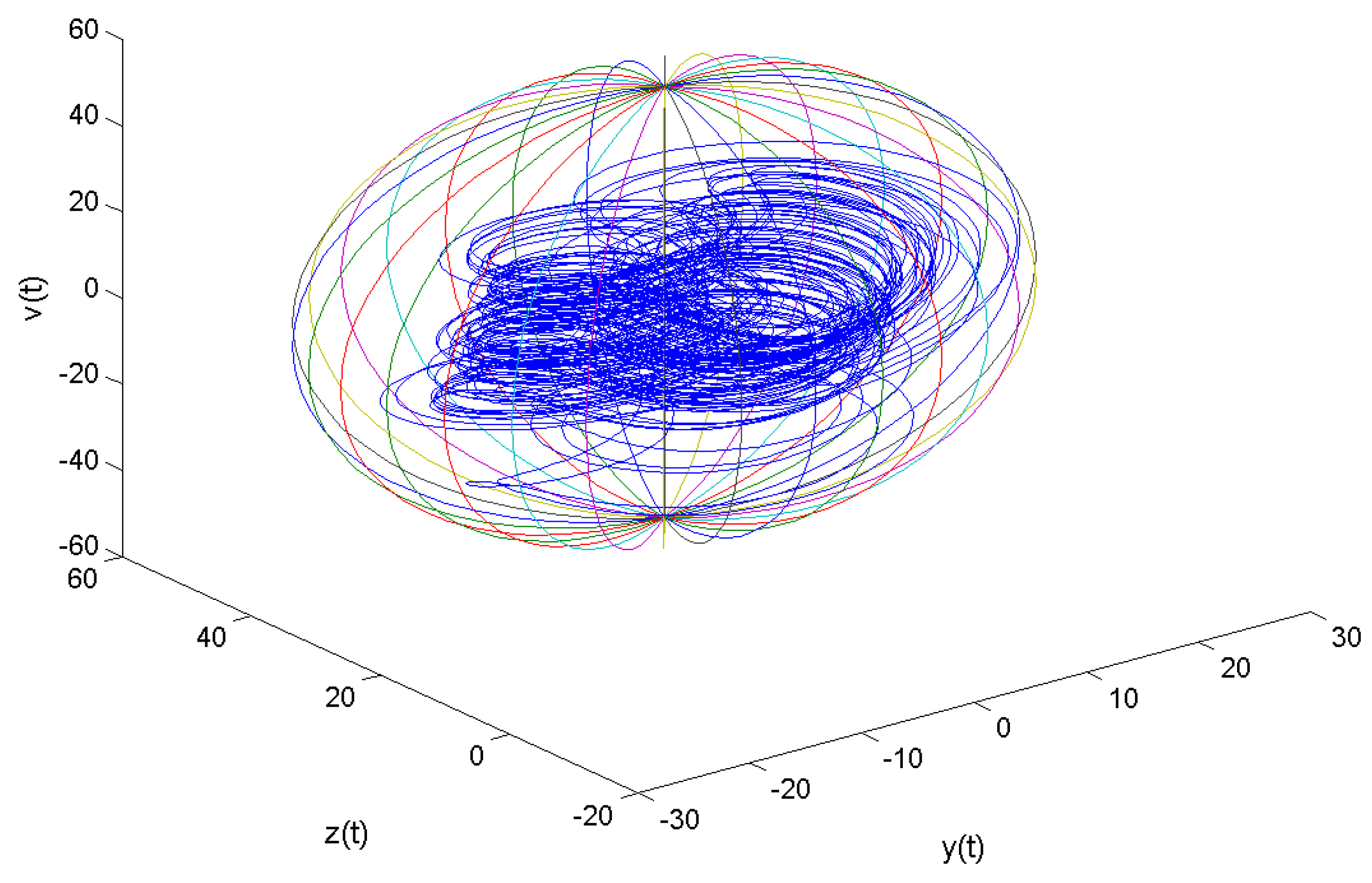
ii. Figure 3 shows that the hyperchaotic attractor of system $\left(1\right)$ is located within $\Phi .$

4. The Globally Exponentially Attractive Set for the New 4D Lorenz-Type Hyperchaotic System

Though Work [25] presents the ultimate bound set and positively invariant set of system $\left(2\right)$, it does not present the trajectories’s rate going from outside the trapping zone to its inside. The following Theorem will find this rate and will also provide a collection of mathematical formulas of global exponential attractive sets for the new 4D Lorenz-type hyperchaotic system.

Theorem 2.

For all $a>0$, $b>0$, $c>0$, $d>0$, $k>0$ and $r>0$, let

$$\begin{array}{cc}\hfill V_{\lambda ,\alpha ,\beta }\left(X\left(t\right)\right)& =\lambda {\left(x-\alpha \right)}^2+k{y}^2+k{\left(z-\frac{\lambda a+kb}{k}\right)}^2+{\left(w-\beta \right)}^2,\hfill \end{array}$$

(27)

where$\begin{array}{cc}\hfill \lambda & >0,\alpha \in \mathbb{R},\beta \in \mathbb{R},X\left(t\right)=\left(x\left(t\right),y\left(t\right),z\left(t\right),w\left(t\right)\right).\hfill \end{array}$

$$\mu =min\left(a,c,d,r\right),R^2=\frac{1}{\mu }\left(\lambda a{\alpha }^2+r{\beta }^2+\frac{d{\left(\lambda a+kb\right)}^2}{k}+\frac{{\left(\beta k-\lambda \alpha a\right)}^2}{kc}\right)$$

Then, an exponential estimation of system $\left(2\right)$ is given by

$$V_{\lambda ,\alpha ,\beta }\left(X\left(t\right)\right)-R^2\le \left(V_{\lambda ,\alpha ,\beta }\left(X\left(t_0\right)\right)-R^2\right)e^{-\mu \left(t-t_0\right)}$$

(28)

Consequently,

$${\Omega }_{\lambda ,\alpha ,\beta }=\left\{\left(x,y,z,w\right)/\lambda {\left(x-\alpha \right)}^2+k{y}^2+k{\left(z-\frac{\lambda a+kb}{k}\right)}^2+{\left(w-\beta \right)}^2\le R^2\right\}$$

(29)

is the globally exponential attractive set of system $\left(2\right).$

Proof of Theorem 2.

Construct the following generalized Lyapunov function

$$\begin{array}{cc}\hfill V_{\lambda ,\alpha ,\beta }\left(X\left(t\right)\right)& =\lambda {\left(x-\alpha \right)}^2+k{y}^2+k{\left(z-\frac{\lambda a+kb}{k}\right)}^2+{\left(w-\beta \right)}^2,\hfill \end{array}$$

(30)

where $\begin{array}{cc}\hfill \lambda & >0,\alpha \in \mathbb{R},\beta \in \mathbb{R},X\left(t\right)=\left(x\left(t\right),y\left(t\right),z\left(t\right),w\left(t\right)\right).\hfill \end{array}$

Computing the derivative of $V_{\lambda ,\alpha ,\beta }\left(X\left(t\right)\right)$ along the trajectory of system $\left(2\right)$, we have

$$\begin{array}{cc}\hfill \frac{d{V}_{\lambda ,\alpha ,\beta }\left(X\left(t\right)\right)}{dt}& =2\lambda \left(x-\alpha \right)x^{\prime }+2ky{y}^{\prime }+2k\left(z-\frac{\lambda a+kb}{k}\right)z^{\prime }+2\left(w-\beta \right)w^{\prime }\hfill \\ \hfill & =2\lambda \left(x-\alpha \right)\left(ay-ax\right)+2ky\left(bx-cy-xz+w\right)+2k\left(z-\frac{\lambda a+kb}{k}\right)\left(xy-dz\right)\hfill \\ \hfill & +2\left(w-\beta \right)\left(-rw-ky\right)\hfill \\ \hfill & =-2a\lambda x^2+2\lambda \alpha ax-2kc{y}^2+2\left(\beta k-\lambda \alpha a\right)y-2kd{z}^2+2d\left(\lambda a+kb\right)z-2r{w}^2+2\beta rw\hfill \\ \hfill & \le -a\lambda x^2+2\lambda \alpha ax-2kc{y}^2+2\left(\beta k-\lambda \alpha a\right)y-kd{z}^2+2d\left(\lambda a+kb\right)z-r{w}^2+2\beta rw\hfill \\ \hfill & =-a\lambda {\left(x-\alpha \right)}^2+a\lambda {\alpha }^2-kc{y}^2-kc{y}^2+2\left(\beta k-\lambda \alpha a\right)y-kd{\left(z-\frac{\lambda a+kb}{k}\right)}^2\hfill \\ \hfill & +\frac{d{\left(\lambda a+kb\right)}^2}{k}-r{\left(w-\beta \right)}^2+r{\beta }^2\hfill \\ \hfill & \le -a\lambda {\left(x-\alpha \right)}^2+a\lambda {\alpha }^2-kc{y}^2+\underset{y\in \mathbb{R}}{max}\left(-kc{y}^2+2\left(\beta k-\lambda \alpha a\right)y\right)\hfill \\ \hfill & -kd{\left(z-\frac{\lambda a+kb}{k}\right)}^2+\frac{d{\left(\lambda a+kb\right)}^2}{k}-r{\left(w-\beta \right)}^2+r{\beta }^2\hfill \end{array}$$

(31)

Since

$$\underset{y\in \mathbb{R}}{max}\left(-kc{y}^2+2\left(\beta k-\lambda \alpha a\right)y\right)=\frac{{\left(\beta k-\lambda \alpha a\right)}^2}{kc},$$

(32)

then, we have

$$\begin{array}{cc}\hfill \frac{d{V}_{\lambda ,\alpha ,\beta }\left(X\left(t\right)\right)}{dt}& \le -a\lambda {\left(x-\alpha \right)}^2-kc{y}^2-kd{\left(z-\frac{\lambda a+kb}{k}\right)}^2-r{\left(w-\beta \right)}^2+a\lambda {\alpha }^2+r{\beta }^2\hfill \\ \hfill & +\frac{d{\left(\lambda a+kb\right)}^2}{k}+\frac{{\left(\beta k-\lambda \alpha a\right)}^2}{kc}\hfill \\ \hfill & \le -\mu V_{\lambda ,\alpha ,\beta }\left(X\left(t\right)\right)+a\lambda {\alpha }^2+r{\beta }^2+\frac{d{\left(\lambda a+kb\right)}^2}{k}+\frac{{\left(\beta k-\lambda \alpha a\right)}^2}{kc}\hfill \\ \hfill & =-\mu \left[V_{\lambda ,\alpha ,\beta }\left(X\left(t\right)\right)-\frac{1}{\mu }\left(a\lambda {\alpha }^2+r{\beta }^2+\frac{d{\left(\lambda a+kb\right)}^2}{k}+\frac{{\left(\beta k-\lambda \alpha a\right)}^2}{kc}\right)\right]\hfill \\ \hfill & =-\mu \left[V_{\lambda ,\alpha ,\beta }\left(X\left(t\right)\right)-R^2\right]\hfill \end{array}$$

(33)

where,

$$\mu =min\left(a,c,d,r\right),R^2=\frac{1}{\mu }\left(\lambda a{\alpha }^2+r{\beta }^2+\frac{d{\left(\lambda a+kb\right)}^2}{k}+\frac{{\left(\beta k-\lambda \alpha a\right)}^2}{kc}\right)$$

(34)

Thus, we obtain

$$V_{\lambda ,\alpha ,\beta }\left(X\left(t\right)\right)-R^2\le \left(V_{\lambda ,\alpha ,\beta }\left(X\left(t_0\right)\right)-R^2\right)e^{-\mu \left(t-t_0\right)}$$

and

$$\underset{t\to +\infty }{lim}{V}_{\lambda ,\alpha ,\beta }\left(X\left(t\right)\right)\le R^2.$$

Consequently,

$${\Omega }_{\lambda ,\alpha ,\beta }=\left\{\left(x,y,z,w\right)/\lambda {\left(x-\alpha \right)}^2+k{y}^2+k{\left(z-\frac{\lambda a+kb}{k}\right)}^2+{\left(w-\beta \right)}^2\le R^2\right\}$$

is the globally exponential attractive set of system $\left(2\right).$ □

Numerical Simulations

i. According to Theorem 2, when $a=12$, $b=23$, $c=1$, $d=2.1$, $k=6$, $r=0.2$, $\lambda =1$, $\alpha =0$ and $\beta =0$ we have

$${\Omega }_{1,0,0}=\left\{\left(x,y,z,w\right)/x^2+k{y}^2+k{\left(z-25\right)}^2+w^2\le 39375\right\}.$$

(35)

is the globally exponential attractive set of system $\left(2\right)$ and we conclude that its trajectories go from outside ${\Omega }_{1,0,0}$ to inside ${\Omega }_{1,0,0}$ at exponential rate.

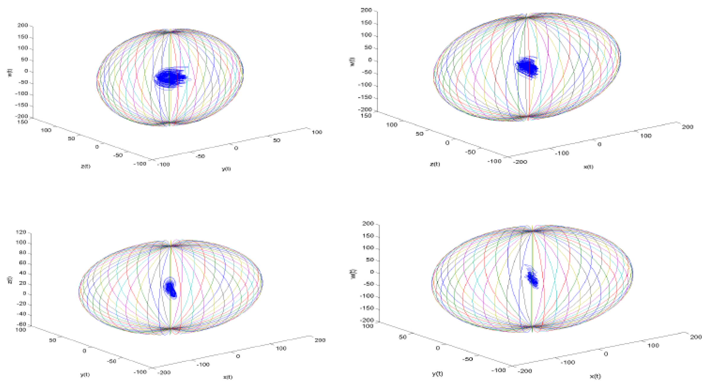
ii. Figure 4 illustrate that the trajectories of system $\left(2\right)$ are restricted in ${\Omega }_{1,0,0}$. That is to say, the system cannot have the equilibrium points, periodic or quasi-periodic solutions, or other chaotic or hyper-chaotic or hidden attractors existing outside the attractive set ${\Omega }_{1,0,0}$.

5. Conclusions

In this paper, we have used analytical optimization, the comparison principle, and generalized Lyapunov function theory to find the ultimate bound set for a new six-dimensional hyperchaotic system and a collection of globally exponentially attractive sets for a new four-dimensional hyperchaotic system. Moreover, we came to the conclusion that the trajectories of the new $4D$ hyperchaotic system move from outside the trapping zone to its inside at an exponential rate. Finally, a few numerical simulations are shown to demonstrate the viability and accuracy of the suggested approach. The obtained results can be applied to chaos control, chaos synchronization, and determining the Lyapunov and Hausdorff dimensions of the studied systems, and this is what we will talk about in more detail in other next works.

References

- Rössler, O.E. An equation for hyperchaos. Phys. Lett. A 1979, 71, 155–157. [Google Scholar] [CrossRef]
- Udaltsov, V.; Goedgebuer, J.; Larger, L.; Cuenot, J.; Levy, P. Communicating with hyperchaos: The dynamics of a DNLF emitter and recovery of transmitted information. Opt. Spectrosc. 2003, 95, 114–118. [Google Scholar] [CrossRef]
- Cenys, A.; Tamaservicius, A.; Baziliauskas, A.; Krivickas, R.; Lindberg, E. Hyperchaos in coupled Colpitts oscillators. Chaos Solitons Fractals 2003, 17, 349–353. [Google Scholar] [CrossRef] [Green Version]
- Vicente, R.; Daudén, J.; Colet, P.; Toral, R. Analysis and characterization of thehyperchaos generated by a semiconductor laser subject to delayed feedbackloop. IEEE J. Quantum Electron 2005, 41, 541–548. [Google Scholar] [CrossRef] [Green Version]
- Arena, P.; Baglio, S.; Fortuna, L.; Manganaro, G. Hyperchaos from cellularnetworks. Electron. Lett. 1995, 31, 250–251. [Google Scholar] [CrossRef]
- Sixiao, K.; Chunbiao, L.; Shaobo, H.; Serdar, ç.; Qiang, L. A memristive map with coexisting chaos and hyperchaos. Chin. Phys. B 2021, 30, 110502. [Google Scholar]
- Hsieh, J.; Hwang, C.; Wang, A.; Li, W. Controlling hyper-chaos of the Rossler system. Int. J. Control 1999, 72, 882–886. [Google Scholar] [CrossRef]
- Jiang, P.; Wang, B.; Bu, S.; Xia, Q.; Luo, X. Hyperchaotic synchronizationin deterministic small-world dynamical networks. Int. Mod. Phys. B 2004, 18, 2674–2679. [Google Scholar] [CrossRef]
- Liao, X.; Fu, Y.; Xie, S.; Yu, P. Globally exponentially attractive sets of the family of Lorenz systems. Sci. China Ser. F 2008, 51, 283–292. [Google Scholar] [CrossRef]
- Kuznetsov, N.; Mokaev, T.; Vasilyev, P. Numerical justification of Leonov conjecture on Lyapunov dimension of Rossler attractor. Commun. Nonlinear Sci. Numer. Simul. 2014, 19, 1027–1034. [Google Scholar] [CrossRef]
- Saberi Nik, H.; Effati, S.; Saberi-Nadjafi, J. Ultimate bound sets of a hyperchaotic system and its application in chaos synchronization. Complexity 2014, 20, 30–44. [Google Scholar]
- Saberi Nik, H.; Golchaman, M. Chaos control of a bounded 4D chaotic system. Neural Comput. Appl. 2014, 25, 683–692. [Google Scholar] [CrossRef]
- Gao, W.; Yan, L.; Saeedi, M.; Saberi Nik, H. Ultimate bound estimation set and chaos synchronization for a financial risk system. Math. Comput. Simul. 2018, 154, 19–33. [Google Scholar] [CrossRef]
- Jian, J.; Zhao, Z. New estimations for ultimate boundary and synchronization control for a disk dynamo system. Nonlinear Anal. Hybrid Syst. 2013, 9, 56–66. [Google Scholar] [CrossRef]
- Karimov, A.; Tutueva, A.; Karimov, T.; Druzhina, O.; Butusov, D. Adaptive generalized synchronization between circuit and computer implementations of the Rössler system. Appl. Sci. 2020, 11, 81. [Google Scholar] [CrossRef]
- Leonov, G.; Bunin, A.; Koksch, N. Attractor localisation of the Lorenz system. Z. Angew. Math. Mech. 1987, 67, 649–656. [Google Scholar] [CrossRef]
- Leonov, G.; Reitmann, V. Attraktoreingrenzung fur Nichtlineare System; Tenbner: Leipzing, Germany, 1987. [Google Scholar]
- Sun, Y. Solution bounds of generalized Lorenz chaotic system. Chaos Solitons Fractals 2009, 40, 691–696. [Google Scholar] [CrossRef]
- Li, D.; Lu, J.; Wu, X.; Chen, G. Estimating the bounds for the Lorenz family of chaotic systems. Chaos Solitons Fractals 2005, 23, 529–534. [Google Scholar] [CrossRef]
- Pogromsky, A.; Santoboni, G.; Nijmeijer, H. An ultimate bound on the trajectories of the Lorenz systems and its applications. Nonlinearity 2003, 16, 1597–1605. [Google Scholar] [CrossRef]
- Wang, P.; Li, D.; Hu, Q. Bounds of the hyper-chaotic Lorenz-Stenflo system. Commun. Nonlinear Sci. Numer. 2010, 15, 2514–2520. [Google Scholar] [CrossRef]
- Rezzag, S. Boundedness of the new modified hyperchaotic Pan System. Nonlinear Dyn. Syst. Theory 2017, 17, 402–408. [Google Scholar]
- Zhang, F.; Xiao, M. Complex dynamical behaviors of Lorenz-Stenflo equations. Mathematics 2019, 7, 513. [Google Scholar] [CrossRef]
- Lingzhi, Y.; Weihong, X.; Wenxin, Y.; Binren, W. Dynamical analysis, circuit implementation and deep belief network control of new six-dimensional hyperchaotic system. J. Algorithms Comput. Technol. 2018, 12, 361–375. [Google Scholar]
- Yuxia, L.; Xuezhen, L.; Guanrong, C.; Xiaoxin, L. A new hyperchaotic Lorenz-type system: Generation, analysis, and implementation. Int. J. Circuit Theory Appl. 2011, 39, 865–879. [Google Scholar]
Figure 1.
Hyperchaotic attractor of system in 2−D spaces with and initial condition .
Figure 2.
Figure 3.
The trajectories of , and of the system are restrained in , where , , , , , and the initial state .
Figure 4.
The trajectories of system are contained in the globally exponential attractive set in different 3−D projection planes, where , , , , , and the initial state .
Publisher’s Note: MDPI stays neutral with regard to jurisdictional claims in published maps and institutional affiliations. |
© 2022 by the authors. Licensee MDPI, Basel, Switzerland. This article is an open access article distributed under the terms and conditions of the Creative Commons Attribution (CC BY) license (https://creativecommons.org/licenses/by/4.0/).
Share and Cite
MDPI and ACS Style
Rezzag, S.; Zhang, F. On the Dynamics of New 4D and 6D Hyperchaotic Systems. Mathematics 2022, 10, 3668. https://doi.org/10.3390/math10193668
AMA Style
Rezzag S, Zhang F. On the Dynamics of New 4D and 6D Hyperchaotic Systems. Mathematics. 2022; 10(19):3668. https://doi.org/10.3390/math10193668
Chicago/Turabian StyleRezzag, Samia, and Fuchen Zhang. 2022. "On the Dynamics of New 4D and 6D Hyperchaotic Systems" Mathematics 10, no. 19: 3668. https://doi.org/10.3390/math10193668
Note that from the first issue of 2016, this journal uses article numbers instead of page numbers. See further details here.