
A Predator–Prey Model with Beddington–DeAngelis Functional Response and Multiple Delays in Deterministic and Stochastic Environments


Abstract
:1. Introduction
2. Deterministic Scenario
2.1. Model Formulation
2.2. The Positivity and Permanence of Solutions
2.3. Existence of Equilibrium Status
2.4. Global Asymptotic Stability
3. Stochastic Scenario
3.1. Model Formulation
3.2. Existence and Stochastic Permanence of Model (4)
3.3. Stability in Distribution
- (1)
- There exists a constant such that .
- (2)
- There exists a non-negative function such that is negative for any
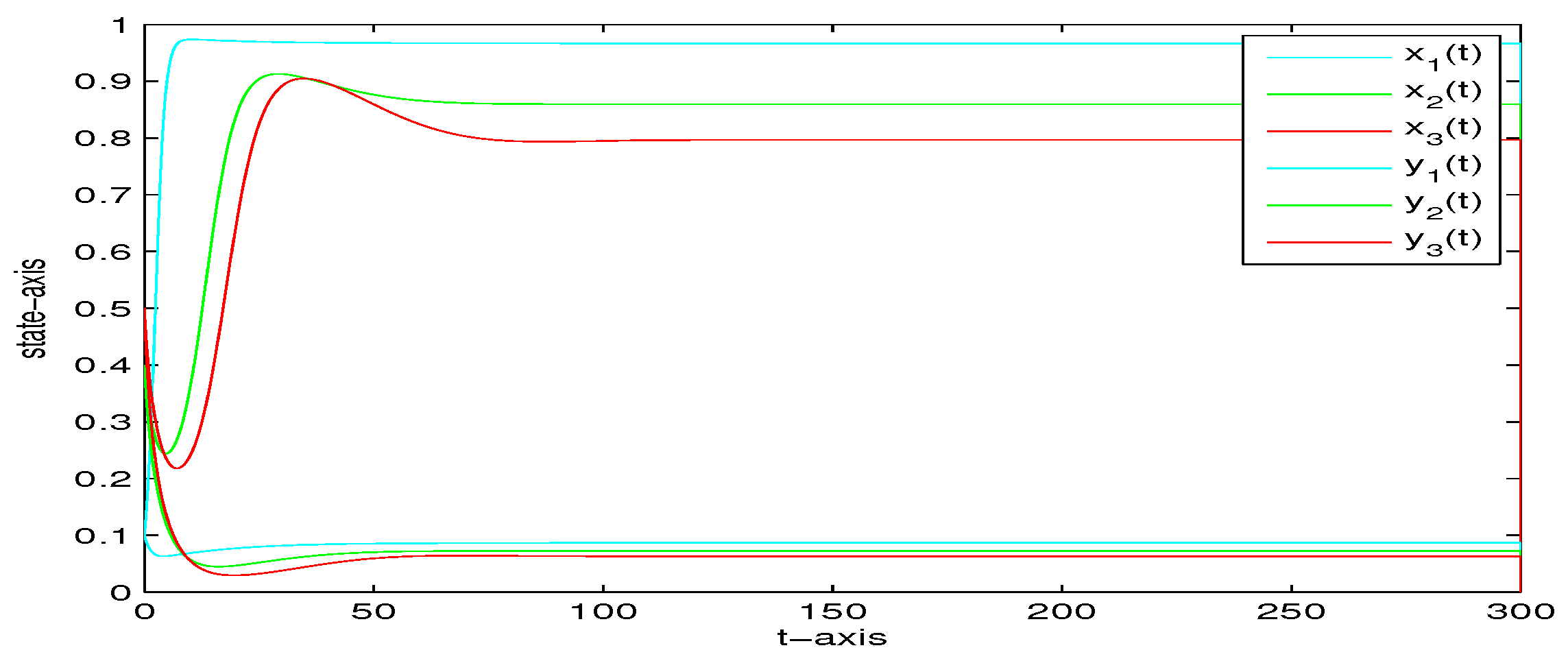
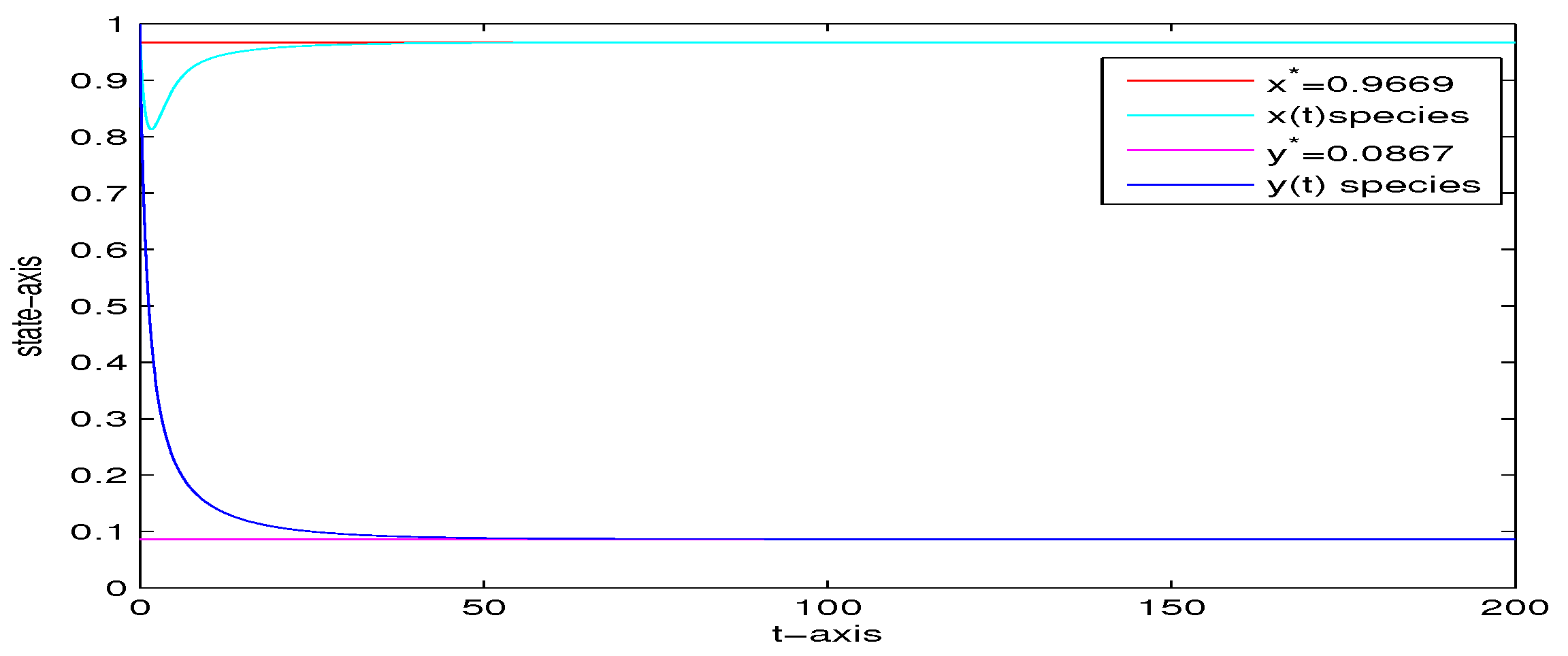
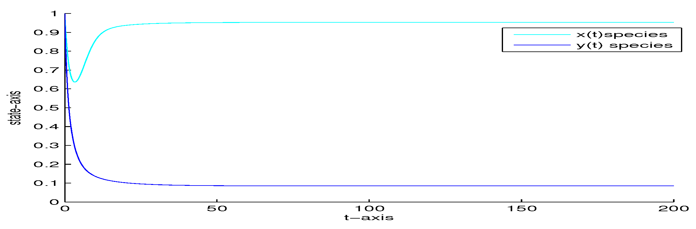
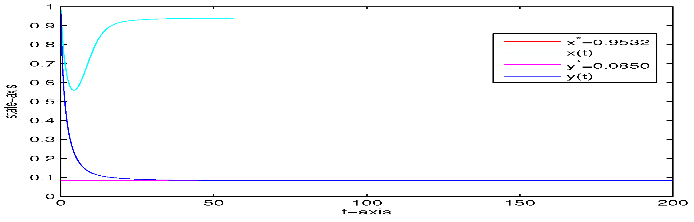
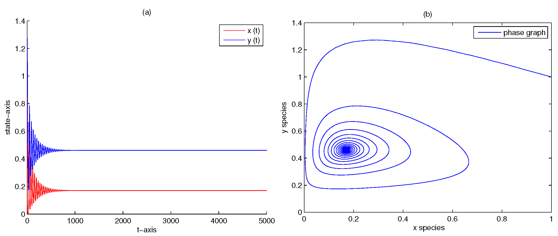
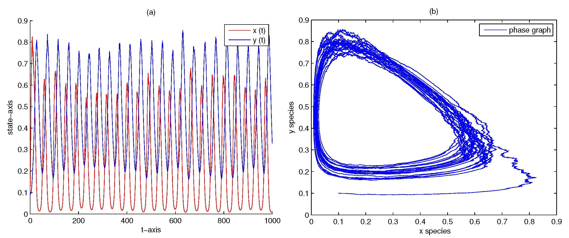
4. Numerical Analysis
5. Conclusions
- Theorems 1 and 2 show the effects of fear on the global stability of Systems (1) and (2), respectively. Remark 2 reveals the effect of delay on system dynamics.
- Lemma 2 gives the representation of the solution of the stochastic differentialEquation (6). By use of the comparison method together with Lemma 2, the existence of the solution of System (4) is proved, which is distinct from the Lyapunov functional methods applied in some existing research [9,15,32].
- Theorem 3 shows theoretically the effects of environmental white noise and fear on the distribution stability.
Author Contributions
Funding
Institutional Review Board Statement
Informed Consent Statement
Data Availability Statement
Acknowledgments
Conflicts of Interest
References
- Volterra, V. Fluctuations in the abundance of a species considered mathematically. Nature 1926, 118, 558–560. [Google Scholar] [CrossRef]
- Holling, C.S. The functional response of predator to prey density and its role in mimicry and population regulation. Mem. Entomol. Soc. Can. 1965, 45, 1–60. [Google Scholar] [CrossRef]
- Shao, Y.F.; Li, Y. Dynamical analysis of a stage structured predator-prey system with impulsive diffusion and generic functional response. Appl. Math. Comput. 2013, 220, 472–481. [Google Scholar] [CrossRef]
- Xu, D.S.; Liu, M.; Xu, X.F. Analysis of a stochastic predator-prey system with modified Leslie-Gower and Holling-type IV schemes. Physica A 2020, 537, 122761. [Google Scholar] [CrossRef]
- Roy, J.; Barman, D.; Alam, S. Role of fear in a predator-prey system with ratio-dependent functional response in deterministic and stochastic environment. BioSystems 2020, 197, 104176. [Google Scholar] [CrossRef] [PubMed]
- Skalski, G.T.; Gilliam, J.F. Functional response with predator interference: Viable aiternative to the Holling type II model. Ecology 2001, 82, 3083–3092. [Google Scholar] [CrossRef]
- Beddington, J.R. Mutual interference between parasites of predators and its effect on searching efficiency. J. Anim. Eccol. 1975, 44, 331–341. [Google Scholar] [CrossRef]
- DeAngelis, D.L.; Goldsten, R.A.; Neill, R. A model for trophic interaction. Ecology 1975, 56, 881–892. [Google Scholar] [CrossRef]
- Xia, Y.X.; Yuan, S.L. Survival analysis of a stochastic predator-prey model with prey refuge and fear effect. J. Biol. Dynam. 2020, 14, 871–892. [Google Scholar] [CrossRef]
- Zanette, L.Y.; Allen, A.F.; Clinchy, M. Percieved predation risk reduces the number of spring songbirds produe per year. Science 2011, 334, 1398–1401. [Google Scholar] [CrossRef]
- Wang, X.; Zanette, L.; Zou, X. Modelling the fear effect in predator-prey interactions. J. Math. Biol. 2016, 73, 1179–1204. [Google Scholar] [CrossRef] [PubMed]
- Elliot, K.H.; Betini, G.S.; Norris, D.R. Fear creats an Alleeeffects: Experimental evidence from seasonal populations. Proc. Biol. Sci. 2017, 284, 20170878. [Google Scholar]
- Panday, P.; Samanta, S.; Pal, N.; Chattopadhyay, J. Delay induced multiple stability switch and chaos in a predator-prey model with fear effect. Math. Comput. Simul. 2020, 172, 134–158. [Google Scholar] [CrossRef]
- Sahoo, D.; Samanta, G.P. Comparison between two tritrophic food chain models with multiple delays and anti-predation effect. Int. J. Biomath. 2021, 14, 2150010. [Google Scholar] [CrossRef]
- Shao, Y. Global stability of a delayed predator-prey system with fear and Holling-type II functional response in deterministic and stochastic environments. Math. Comput. Simul. 2022, 200, 65–77. [Google Scholar] [CrossRef]
- Wang, Y.; Zou, X. On a predator-prey system with digestion delay and anti-predation strategy. J. Nonlinear Sci. 2020, 30, 1579–1605. [Google Scholar] [CrossRef]
- Xiao, Y.; Chen, L. Modelling and analysis of a predator-prey model with disease in the prey. Math. Biosci. 2001, 171, 59–82. [Google Scholar] [CrossRef]
- Kuang, Y. Delay Differential Equations with Applications in Population Dynamics; Academic Press: New York, NY, USA, 1993. [Google Scholar]
- Upadhyay, R.K.; Mukhopadhyay, A.; Iyengar, S.R. Influence of environmental noise on the dynamics of a realistic ecological model. Fluct. Noise Lett. 2007, 7, 61–77. [Google Scholar] [CrossRef]
- Liu, M.; Wang, K. Stochastic Lotka-Volterra systems with Lévy noise. J. Math. Anal. Appl. 2014, 410, 750–763. [Google Scholar] [CrossRef]
- Zhao, Y.; Yuan, S. Stability in distribution of a stochastic hybrid competitive Lotka-Volterra model with Lévy jumps. Chaos Solitons Fractals 2016, 85, 98–109. [Google Scholar] [CrossRef]
- Mao, X. Stochastic Differential Equations and Applications; Horwood Publishing: Chichester, UK, 1997. [Google Scholar]
- Liu, M.; Wang, K. Global asymptotic stability of a stochastic Lotka-Volterra model with infinite delays. Commun. Nonlinear Sci. Numer. Simul. 2012, 17, 3115–3123. [Google Scholar] [CrossRef]
- Liu, Q. The effects of time-dependent delays on global stability of stochastic Lotka-Volterra competitive model. Physica A 2015, 420, 108–115. [Google Scholar] [CrossRef]
- Has’minskii, R.Z. Stochastic Stability of Differential Equations; Sijthoff Noordhoff: Alphen annden Rijn, The Netherlands, 1980. [Google Scholar]
- Song, X.Y.; Chen, L.S. Optimal harvesting and stability with stage structure for a two species competitive system. Math. Biosci. 2001, 170, 173–186. [Google Scholar] [CrossRef]
- May, R. Stability in randomly fluctuating deterministic environments. Am. Nat. 1973, 107, 621–650. [Google Scholar] [CrossRef]
- Mao, X.; Yuan, C.; Zou, J. Sttochastic differential delay equations of population dynamics. J. Math. Anal. Appl. 2005, 304, 296–320. [Google Scholar] [CrossRef]
- Huang, Y.; Liu, Q.; Liu, Y.L. Global asymptotic stability of a general stochastic Lotka-Volterra system with delays. Appl. Math. Lett. 2013, 26, 175–178. [Google Scholar] [CrossRef]
- Das, A.; Samanta, G.P. Modelling the fear effect in a two-species predator-prey system under the influence of toxic substances. Rend. Circ. Mat. Palermo Ser. 2 2021, 70, 1501–1526. [Google Scholar] [CrossRef]
- Higham, D.J. An aigorithmic introduction to numerical simulations of stochastic differential equations. SIAM Rev. 2001, 43, 525–546. [Google Scholar] [CrossRef]
- Kong, W.L.; Shao, Y. The long time behavior of equilibrium status of a predator-prey system with delayed fear in deterministic and stochastic scenarios. J. Math. 2022, 2022, 3214358. [Google Scholar] [CrossRef]
- Waezizadeha, T.; Mehrpooya, A.; Rezaeizadehc, M.; Yarahmadiand, S. Mathematical models for the effects of hypertension and stress on kidney and their uncertainty. Math. Bios. 2018, 305, 77–95. [Google Scholar] [CrossRef]
- Brehme, M.; Koschmieder, S.; Montazeri, M.; Copland, M.; Oehler, V.G.; Radich, J.P.; Brmmendorf, T.H.; Schuppert, A. Combined population dynamics and entropy modelling supports patient stratification in Chronic cyeloid leukemia. Sci. Rep. 2016, 6, 24057. [Google Scholar] [CrossRef] [PubMed] [Green Version]


| Parameter | Biological Meaning |
|---|---|
| Intrinsic growth rate of prey | |
| Natural mortality rate of predator | |
| Intra-specific competition coefficient of prey | |
| Density dependence rate of predator | |
| P | Maximal relative increase of predation |
| Q | Conversion factor |
| Half-saturation constant | |
| Magnitude of interference among predators | |
| f | Fear effect of prey induced by predator |
| Parameters | Stability of Equilibria | Simulation Figures | |||
|---|---|---|---|---|---|
| Fear | Time Delays | Stochastic Effect | Equilibria | ||
| 0 | 0 | 0 | yes | Figure 2 | |
| 5 | 0 | 0 | yes | Figure 3 | |
| 5 | 0.2 | 0 | yes | Figure 4 | |
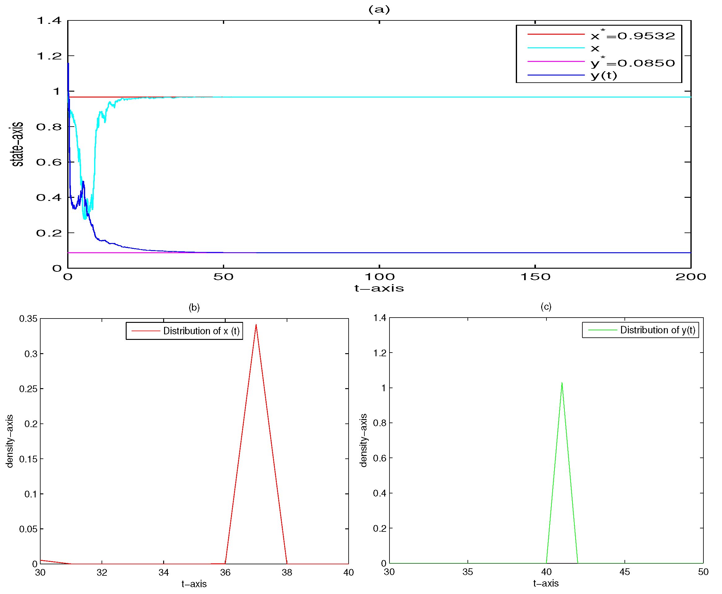
| 5 | 0.2 | 1 | yes | Figure 5 | |
| Parameters | Stability of Equilibria | Simulation Figures | |||
|---|---|---|---|---|---|
| Fear | Time Delay | Stochastic Effect | Equilibria | ||
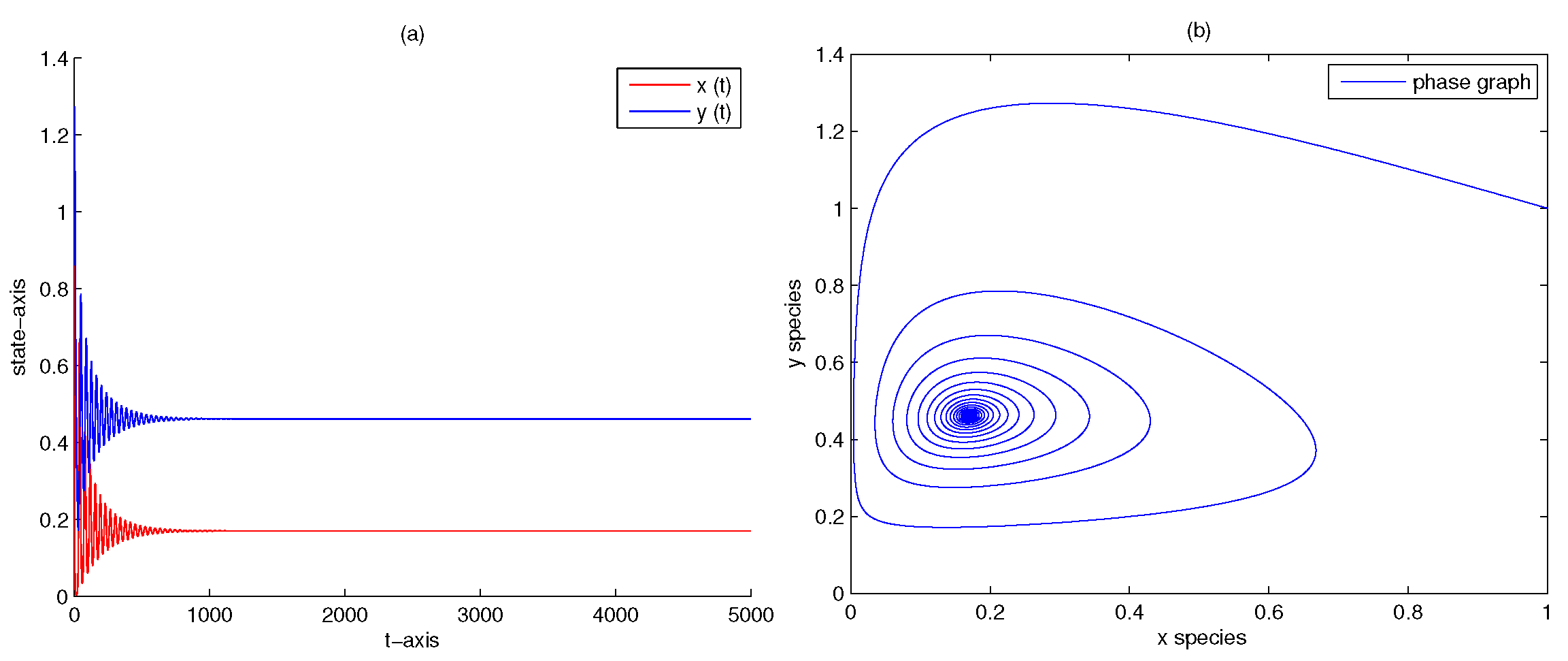
| 5 | 0 | 0 | yes | Figure 6 | |
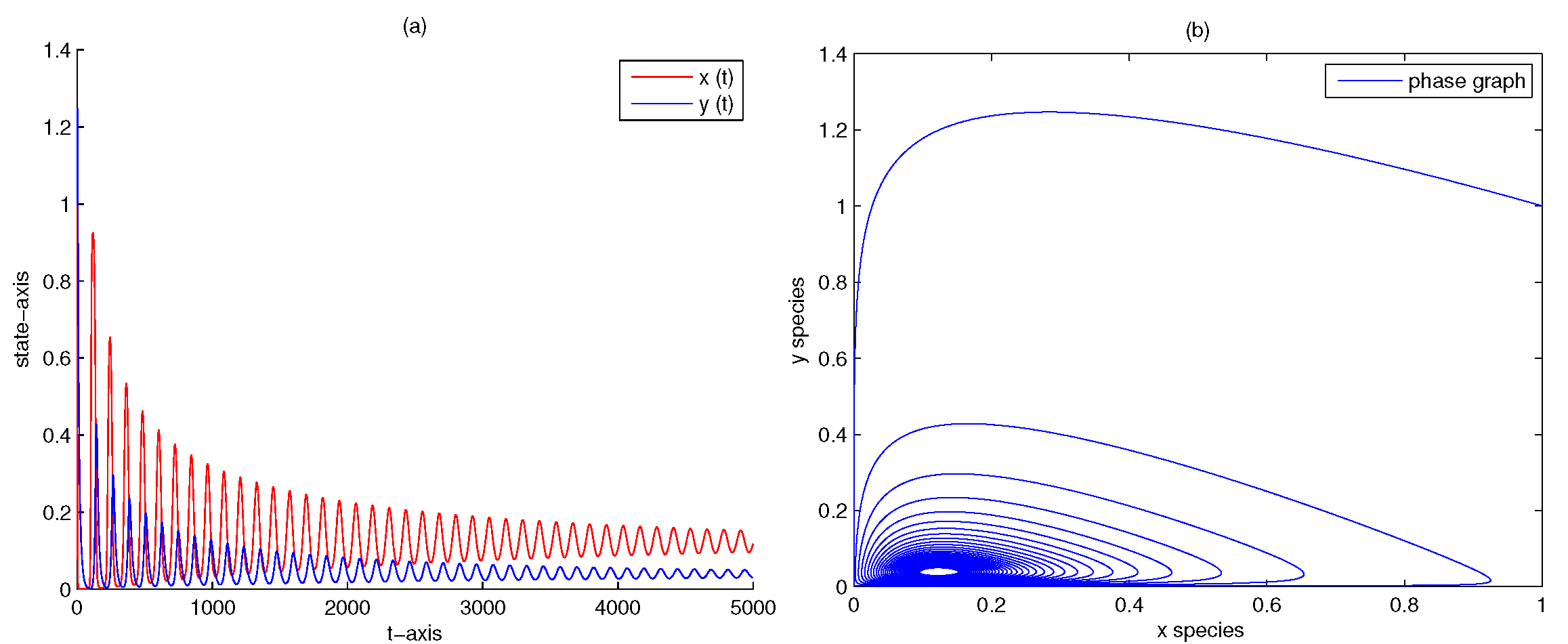
| 1000 | 0 | 0 | no | Figure 7 | |
| 5 | 0.5 | 0 | no | Figure 8 | |
| 5 | 0 | 0.02 | yes | Figure 9 | |
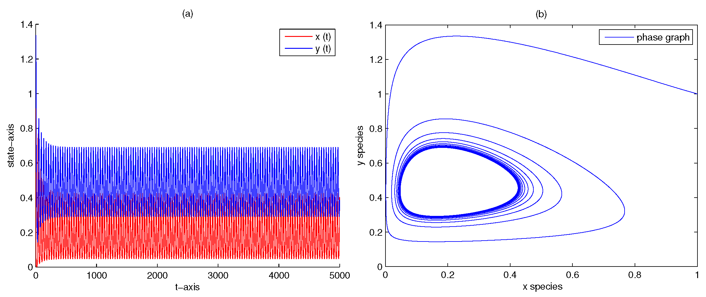
| 5 | 0 | 0.5 | no | Figure 10 | |
| Parameters | Stability Conditions | ||
|---|---|---|---|
| Fear | Stochastic Effect | Time Delay | |
| no | no | no | |
| no | no | yes | |
| no | yes | no | |
| no | yes | yes | |
| yes | no | no | |
| yes | no | yes | |
| yes | yes | no | |
| yes | yes | yes | |
Publisher’s Note: MDPI stays neutral with regard to jurisdictional claims in published maps and institutional affiliations. |
© 2022 by the authors. Licensee MDPI, Basel, Switzerland. This article is an open access article distributed under the terms and conditions of the Creative Commons Attribution (CC BY) license (https://creativecommons.org/licenses/by/4.0/).
Share and Cite
Shao, Y.; Kong, W. A Predator–Prey Model with Beddington–DeAngelis Functional Response and Multiple Delays in Deterministic and Stochastic Environments. Mathematics 2022, 10, 3378. https://doi.org/10.3390/math10183378
Shao Y, Kong W. A Predator–Prey Model with Beddington–DeAngelis Functional Response and Multiple Delays in Deterministic and Stochastic Environments. Mathematics. 2022; 10(18):3378. https://doi.org/10.3390/math10183378
Chicago/Turabian StyleShao, Yuanfu, and Weili Kong. 2022. "A Predator–Prey Model with Beddington–DeAngelis Functional Response and Multiple Delays in Deterministic and Stochastic Environments" Mathematics 10, no. 18: 3378. https://doi.org/10.3390/math10183378