1. Introduction
Bone is a living tissue that can adapt its apparent density and internal microstructure (through the process called bone remodelling), and its shape and external dimensions (through bone modelling) as a response to different mechanical and biological stimuli. Regarding the former, it has been hypothesized that one of the goals of bone remodelling is to maintain bone as an optimal structure that supports the loads with the minimum weight [
1]. Thus, bone density, and consequently, stiffness, are high in overloaded regions and low in regions with a low stress level. In other words, there is a direct relationship between density and stresses. Many bone remodelling models (BRM) have been proposed in the literature to quantify this relationship [
1,
2,
3,
4,
5].
These BRM have been very often used to estimate the density distribution in bones from the loads they are subjected to, mainly in the human femur [
6,
7], but also in other bones such as the mandible [
8]. This problem, that we will name here
Density Prediction Through Bone Remodelling (DPTBR), is usually approached through the following iterative process:
Assign an initial uniform density distribution to the bone under study.
Apply the loads and boundary conditions to a Finite Element (FE) model of the bone and calculate the stresses/strains at every point of the mesh.
Apply the BRM to relate the stress/strain state with the new density [
9] or with the change in density [
1,
2,
3,
4,
5], and then update the density at each point.
Update the stiffness tensor at each point based on the new density. Go back to step 2 to start a new iteration.
This iterative process is repeated until convergence of the density distribution is achieved, which usually resembles the real one with good accuracy. The BRM can be applied following two approaches, as mentioned above in step 3. In an evolutionary model, the stress/strain state determines the local change in apparent density,
:
where
S is a certain mechanical stimulus related to the stress/strain state. This approach is based on the Mechanostat Theory [
10], which is behind most of the BRM. This theory hypothesizes that bone adapts itself to overloads by increasing its apparent density and adapts to disuse states by decreasing it. Overload and disuse are defined in the Mechanostat Theory by certain strain ranges. The theory also establishes the existence of a so-called “lazy zone”, a strain range between disuse and overload, for which no evident change in apparent density is observed or, at least, it is not significant. Implementing this approach in DPTBR problems has a major drawback, as the uniqueness of the solution is not guaranteed. This path dependence occurs due to the implementation of the lazy zone [
11], and the final density distribution depends on the initially assumed distribution.
Recently, we have proposed a non-evolutionary strategy to solve DPTBR problems [
9]. Instead of calculating the rate of change in density as a function of the stimulus, we calculated a priori a relationship between the stimulus
S and the density achieved at the equilibrium (see Equation (
2)) and used that relationship to assign the density to an element as a function of the local stimulus. Since this stimulus can, in turn, change with density (through the stiffness), an iterative process is still required, but the number of iterations needed to achieve convergence is much lower. Notwithstanding, the uniqueness of the solution is not guaranteed in this case. The only advantage of this approach is its higher speed of convergence.
On the other hand, the non-evolutionary approach is not suitable to predict the changes in density in a bone subjected to changes in its biomechanical environment. The evolutionary approach is preferable in this case, as it allows a real-time simulation of those changes. However, to this end, it is very important to start from a realistic initial density distribution, in order to avoid the path dependence of the solution previously mentioned.
The stimulus
S is the variable that drives bone remodelling and must comprise biological and mechanical factors. Focusing on the latter, the amount of damage has been used as the stimulus (or a part of it) in targeted bone remodelling models [
12,
13,
14,
15]. This is based on the hypothesis that one goal of bone remodelling is to repair the microstructural damage accumulated in the bone matrix by daily activity. Other models simply apply the Mechanostat Theory to account for disuse and overload and the influence of these states on bone adaptation. To this end, these models have used a stimulus that measures the intensity of the loads, with the strain energy density (SED) being the most commonly used variable to account for that intensity (see [
1,
2,
3,
4,
5], among many others). However, in the original Mechanostat Theory, the disuse, lazy zone and overload states were defined in terms of strain; thus, establishing the hypothesis that strain is the magnitude driving the bone response. In such case, after a change in load that could alter the level of strain, the bone microstructure (and consequently, stiffness) must be regulated to return to the homeostatic situation [
12].
In this work, we will focus on the mechanical part of the stimulus—the main objective being to study which is the best variable among a series of candidates to account for the mechanical feedback in bone remodelling models. We will discuss which is the best mechanical stimulus, or equivalently, which is the best predictor of bone density, either for an evolutionary or a non-evolutionary approach. For this purpose, we have analysed the stress and strain distributions in a human femur using a FE model and the loads extracted from a gait analysis performed on the same individual, from whom we have also estimated the bone density distribution from a CT scan. Several mechanical variables calculated from the stress and strain tensors throughout the gait cycle have been proposed as candidates for the mechanical stimulus (or predictors) and will be correlated with the density distribution.
This paper is organised as follows: In
Section 2.1, we provide a description of the gait analysis performed to estimate the loads acting on the femur during walking. In
Section 2.2, we describe the image analysis of CT scans of a human femur, which were performed to obtain its bone density distribution. In
Section 2.3, we briefly describe the methodology to estimate the stiffness tensor at every point of the femur based on the density distribution. In that section, we focus on the case that considers bone as an isotropic material, while through
Section 2.4,
Section 2.5 and
Section 2.6, we develop the methodology to estimate that stiffness tensor when bone is considered anisotropic. In
Section 2.7, we briefly describe how the gait cycle was simulated with a FE model. The correlation coefficients used to evaluate the relationship between bone density and the variables used as candidates for mechanical stimuli (or predictors) are defined in
Section 2.8. In
Section 2.9, we define those predictors. In
Section 3, we provide the correlations between the bone apparent density and the proposed predictors. We discuss the results of these correlations in
Section 4 and highlight the conclusions of this study in
Section 5. Finally, the Appendices contain a more detailed description of the procedures used in the
Section 2.
2. Materials and Methods
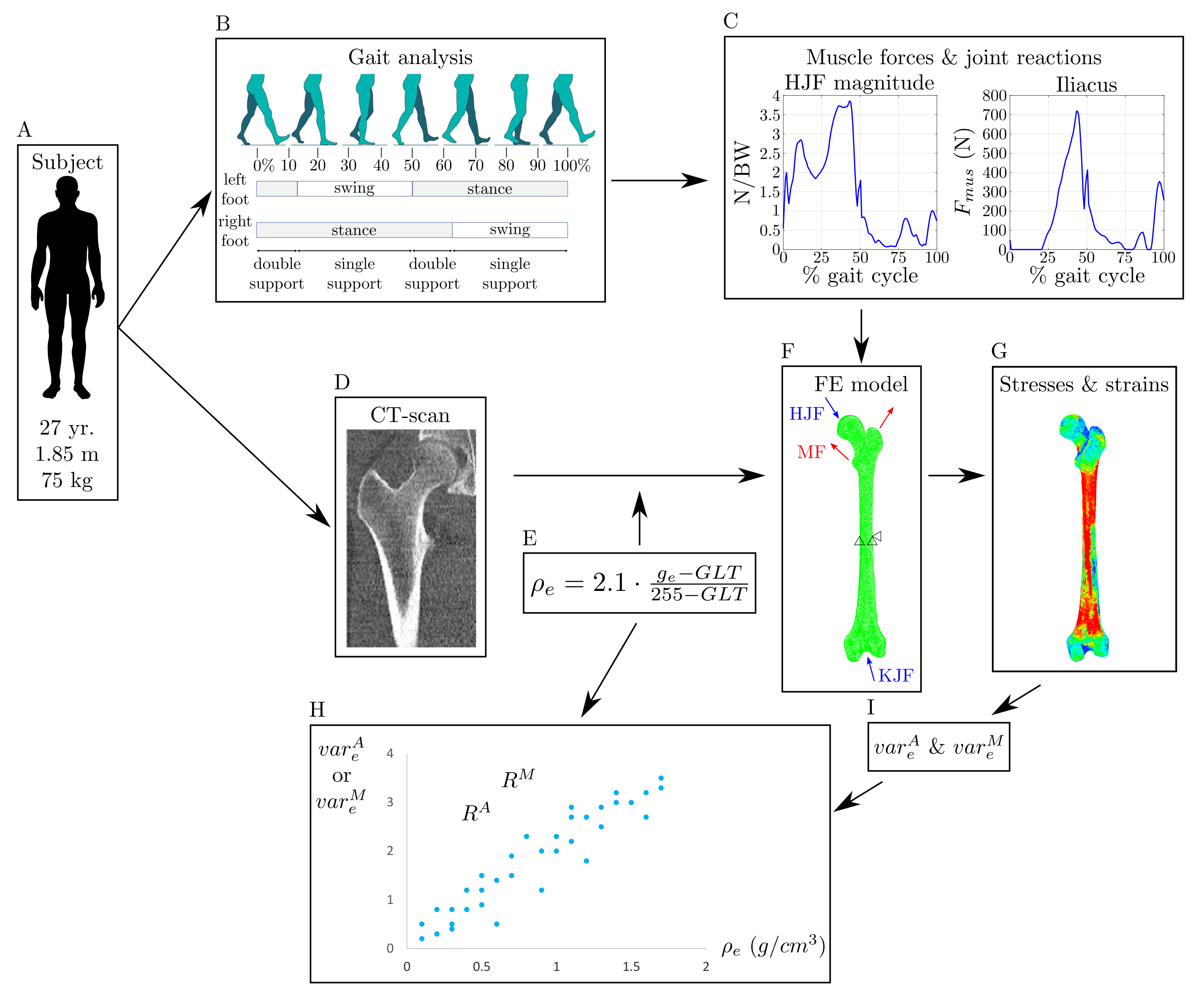
The procedure followed here is summarised in
Figure 1 and is explained as follows: First, a gait analysis was performed to estimate the forces exerted by those muscles inserted in the femur and joint reactions at the knee and the hip in the subject under study. A CT scan of the subject’s femur was taken and the greyscale value was related to the bone apparent density using a linear relationship. With this, a FE model of the femur was built and the loads, estimated through a gait analysis performed on the same subject, were applied to the FE model in order to obtain the distribution of stresses and strains throughout the gait cycle. A set of variables, defined in
Section 2.7 and
Section 2.9, was assessed from the temporal evolutions of stresses and strains. Finally, the bone apparent density estimated from the CT scan was correlated with these variables.
2.1. Gait Analysis and Subject Data
The gait analysis was performed at the Motion Analysis Laboratory of the Department of Mechanical Engineering and Manufacturing of the Universidad de Sevilla. A Vicon®system of 12 infra-red cameras was used to record motion at a frequency of 100 Hz along with 2 AMTI force platforms to record the ground reaction forces at a frequency of 1000 Hz. The marker placement protocol employed was the modified Cleveland protocol [
16].
The subject under study was an adult male of 27 years old, with no reported pathologies, 1.85 m tall and weighing 75 kg, who walked at a freely chosen forward speed. The participant signed an informed consent form prior to the recording of the measurements. The study protocol was approved by a medical ethics committee through the Andalusian Biomedical Research Ethics Platform (approval number 20151012181252).
The recorded experimental data were processed using OpenSim software [
17]. The biomechanical model implemented was the
Gait2392, available in the OpenSim library. This model was developed to perform 3D gait analysis and consists of 23 degrees of freedom and 92 actuators that simulate the action of muscle forces. However, for the sake of simplicity, the subtalar and metatarsophalangeal joints were blocked in this work, so that the foot was considered a single biomechanical segment. The model was scaled to fit the subject’s morphology from the recorded experimental data. The mass ratio of each segment was assumed constant during scaling. In this model, muscle attachment points were placed where OpenSim locate them by default, using numerical approximation [
18] of cadavers’ data [
19,
20].
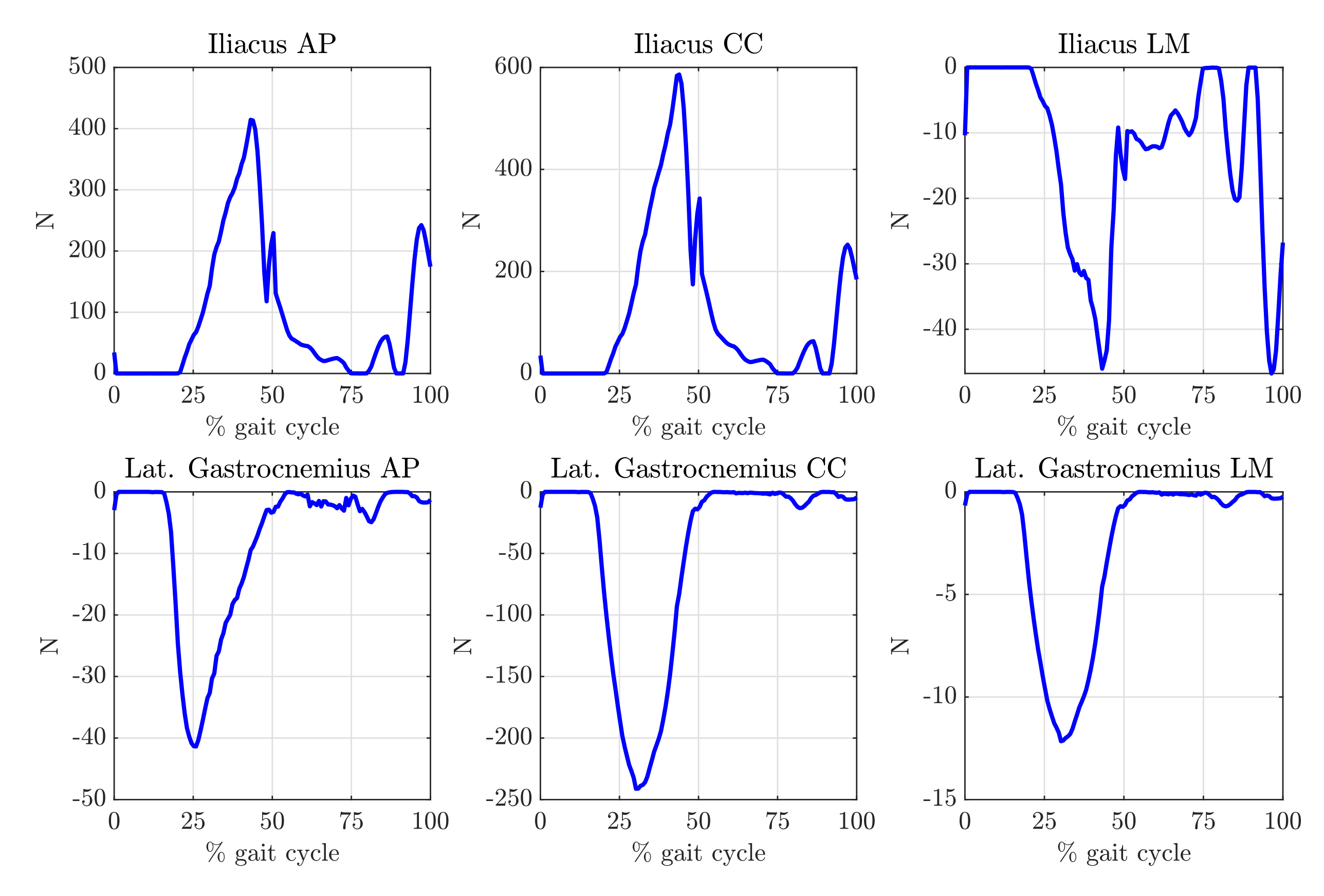
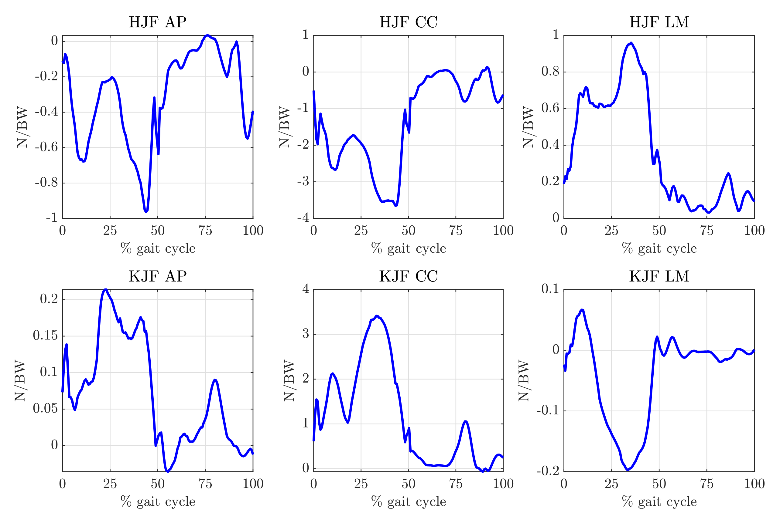
The forces applied to the FE model were obtained in two steps. First, the inverse dynamic problem was solved using the kinetics experimental data recorded in the laboratory. From these results, the time evolutions of the muscle forces were calculated solving a force-sharing problem through a static optimisation algorithm that considered the dynamics of muscle contraction and activation [
17,
21]. The results were collected for those muscles inserted in the femur and are provided in the
Supplementary Materials. Additionally, joint reaction forces at the hip and knee were estimated using the algorithm proposed by Steele et al. [
22]. A detailed description of this procedure is included in
Appendix B.
2.2. CT Scan of the Femur, FE Model and Density Distribution
A CT scanner (LightSpeed16, GE Medical Systems, Milwaukee, WI, USA; 120 kVp, reconstructed with bone Plus kernel, 1.25 mm slice thickness) was used to estimate bone density on the right femur of the same individual on which the gait analysis was conducted. The software Abaqus (version 2020, SIMULIA, Dassault Systémes, Madrid, España) was used to run FE analysis. The 3D geometry of the femur was reconstructed from the CT scan and meshed with 4-node linear tetrahedral elements (C3D4 in Abaqus element library). The final mesh consisted in 339,168 elements and 64,757 nodes. In order to check the convergence of the FE solution, we compared the results with a different mesh, built with 10-node quadratic tetrahedral elements (C3D10). This new mesh was obtained from the previous one by simply placing mid-side nodes in the edges of the former elements, resulting—obviously—in the same number of elements and 480,480 nodes.
To assign a value of density to each element of the mesh, a linear relationship between the greyscale value and the bone apparent density was used, as in [
23,
24,
25,
26]:
where
and
are the greyscale value and the density estimated for element
e, respectively. Two pairs of greyscale–density values are needed to define the linear relationship (constants
A and
B). These points are usually obtained through calibration of the CT scan. However, this calibration was not available in our case, and therefore, we needed to make two assumptions. Thus, as the first pair, an apparent density value of 2.1 g/cm
[
4] was assigned to the maximum greyscale value of the CT scan (255), i.e., to the densest cortical bone. The second point chosen was that corresponding to a null bone apparent density, which is sometimes called a grey level (or greyscale) threshold (GLT). It can be seen in Equation (
4) that
for
. This lower limit is usually made to correspond to bone marrow, which was assumed here to be placed inside the diaphyseal canal. However, the greyscale value inside the canal varied in the range 70–90, thus, making it impossible to assign a unique and reliable value to GLT. For this reason, three cases were studied, assuming different values for GLT, namely: 70, 80 and 90. This uncertainty in the choice of GLT affects the slope of the linear relationship, which is then:
The greyscale distribution was mapped from the CT scan to the FE mesh using the software
Bonemat, and Equation (
3) was used to convert the greyscale value into bone apparent density. Those elements with a greyscale value below GLT were assigned a very small density (0.001 g/cm
), thus, yielding a negligible—although, not null—stiffness, something necessary to avoid convergence problems.
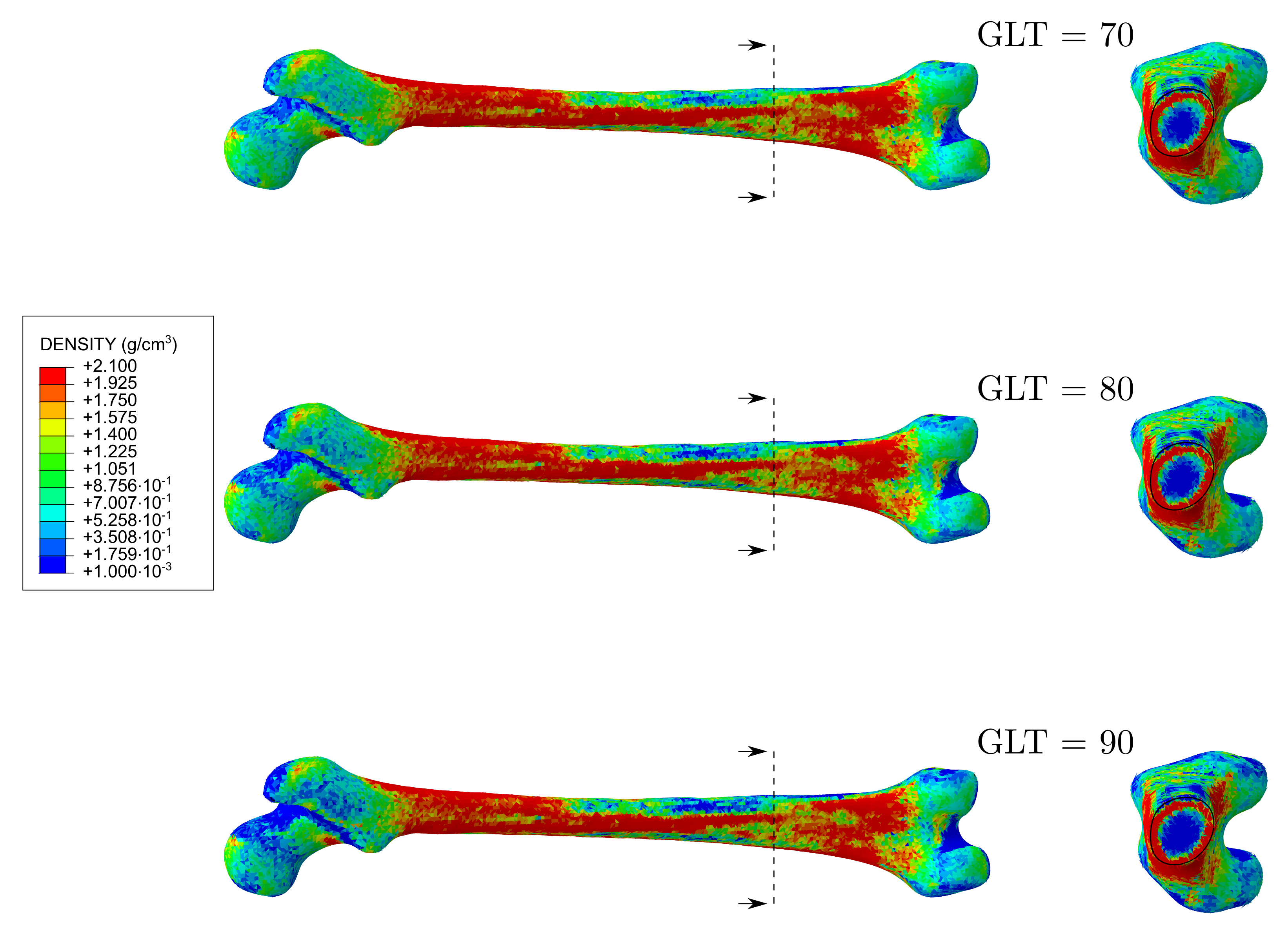
Figure 2 shows the distributions of density obtained for the three GLT. It can be seen that those three GLT led to distributions of the estimated density which are similar, in general, with the exception of the proximal region and the thickness of the cortical layer in the diaphysis. As GLT rises, the volume identified as marrow increases, and this makes GLT = 90 produce a thinner cortical layer and a slightly underestimated density in the proximal region. Nonetheless, it can be noted in
Figure 2 that the uncertainty introduced in the density distribution by GLT is not too important, in the range of 70–90. Moreover, we will show later that the conclusions of this study are the same regardless of the choice of GLT.
The external boundary of the bone was not perfectly defined in some slices of the CT scan where the cortex was too thin, since the average greyscale value between the background and the periosteum produced a cortex of intermediate density. For this reason, the model was covered with a layer of shell elements to simulate the cortex, with a thickness of 1 mm, a Young’s modulus equal to 19 GPa [
27] and a Poisson’s ratio
= 0.32 [
28].
2.3. Estimation of the Stiffness Tensor
Isotropic and anisotropic models were considered. In the former, the stiffness tensor of bone at each material point can be estimated through the density obtained from the CT scan, by using one of the numerous correlations between the elastic constants and the apparent density that can be found in the literature. For example, Jacobs proposed the following [
28]:
Hernandez et al. [
29] proposed another correlation for
E, based on the ash fraction,
(a variable used to measure the mineral content of bone tissue), and on the bone volume fraction (or bone volume per total volume),
. If we express
, with
and
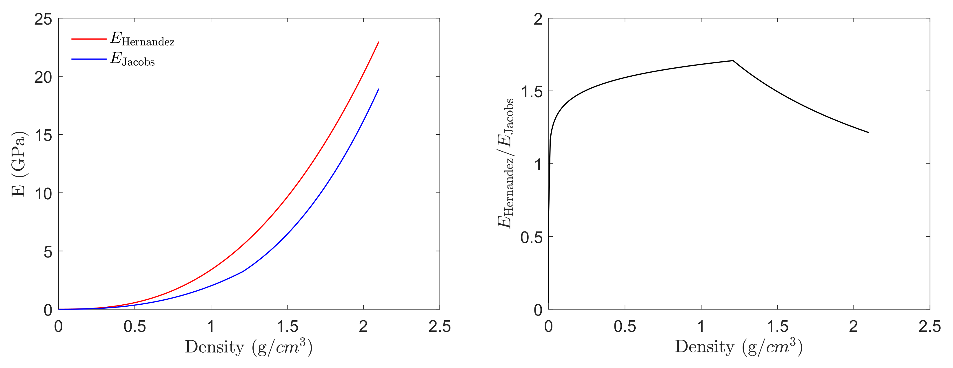
being the apparent density and the tissue density, respectively, then the correlation proposed by Hernandez et al. reads:
If typical values of ash fraction
and tissue density
[
29] are used, Equation (
6) becomes:
which produces an estimation of the Young’s modulus up to 70% higher than Equation (5a) depending on the density (see
Figure 3). Each correlation was used in the corresponding isotropic model, named, respectively,
IsoJ (Equation (5a)) and
IsoH (Equation (
7)) after Jacobs and Hernandez. A constant Poisson’s ratio
was used in conjunction with Equation (
7) in model
IsoH.
Bone is actually an anisotropic material with a dependence of the mechanical properties on the direction and the type of tissue. Particularly, cortical bone is usually modelled as a transversely isotropic material [
30] and trabecular bone as an orthotropic material [
31]. Consequently, its anisotropy must be taken into account in the estimation of the stiffness tensor, and so was carried out in the anisotropic model, named here
AnisoH (note that the H refers to the fact that the anisotropic model relies on Hernandez correlation, as explained later in
Section 2.4).
Some bone remodelling models have been proposed to predict not only the adaptation of bone apparent density but also of its anisotropy [
4,
5]. The model developed by Doblaré and García [
4] was also used to predict the distribution of anisotropy in the same manner as DPTBR simulations are used to predict the distribution of bone density. In fact, these authors predicted both distributions simultaneously. The starting point was an isotropic material with a uniform distribution of density. Their BRM adapted bone density and anisotropy, the latter through the fabric tensor, and both variables were used to update the stiffness tensor. Convergence was deemed when both density and anisotropy remained constant between simulations. A brief summary of this model is provided next, in
Section 2.4.
Given that DPTBR simulations were shown to be path-dependent [
11], we estimated the density distribution from the CT scan and used the bone remodelling model developed by Doblaré and García [
4] to estimate the anisotropy. This required a slight variation of the original model, explained in
Section 2.5. Besides, another variation of the original model was used to account for time-varying loads, such as walking. This variation was introduced by Ojeda [
32] and is presented in
Section 2.6.
The objective of comparing the three models referred to above (IsoJ, IsoH and AnisoH) was to rule out that the assumption made for the constitutive model is forcing a certain correlation between the density and the predictors.
2.4. Anisotropic Bone Remodelling Model Based on Continuum Damage Mechanics—Model by Doblaré and García
A brief description of the anisotropic bone remodelling model developed by Doblaré and García [
4] is given next. Consulting the original paper is advised for a more detailed description of the model. This model is an extension to the anisotropic case of the model developed by Beaupré et al. [
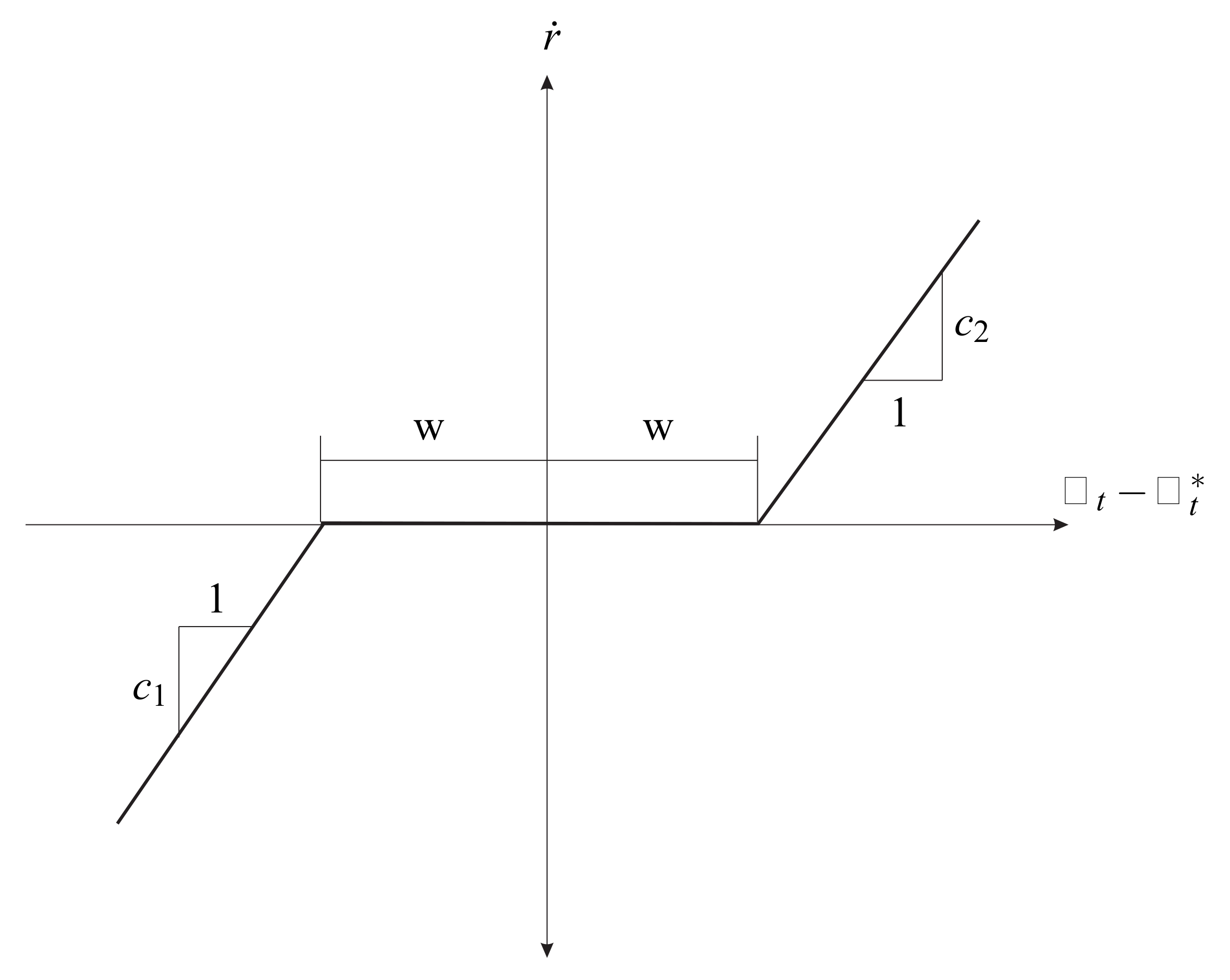
3]. It applies the Mechanostat Theory by defining a stepwise linear relationship between the mechanical stimulus,
, and the bone formation/resorption rate,
(see
Figure 4). The reference value of the stimulus,
defines a region of width 2w called lazy zone (analogous to the “adapted-window” of the Mechanostat Theory), where no net change of bone density is produced. The value of
determines the temporal evolution of apparent density,
. In turn, apparent density determines the variation of the Young’s modulus through correlations such as (5a) or (
7).
The model developed by Doblaré and García was based on the theory of Continuum Damage Mechanics (CDM), where the stiffness tensor of the damaged material,
C, is obtained from the tensor of the the non-damaged material,
, and damage:
where
D is the damage variable, null for an intact material and equal to 1 for a completely damaged or failed material. In the extension of CDM to the anisotropic case introduced by Cordebois and Sideroff [
33], the scalar damage
D is replaced with a damage tensor
and the resulting material is orthotropic, with the principal directions of orthotropy aligning with the principal axes of the damage tensor
. Damage is understood as a measure of porosity and the directionality of that porosity and both are incorporated into the model jointly, by following the idea suggested by Cowin [
34] for the fabric tensor,
. Therefore, the undamaged material is an ideal situation of a perfectly isotropic bone with null porosity. The damage and fabric tensors are related by:
with
being the second order identity tensor. Equation (
9) leads to the following relationship between the components of the compliance tensor in the principal directions and the eigenvalues of the fabric tensor,
:
where
and
are, respectively, the Young’s modulus and Poisson’s ratio of the bone with no porosity. These values can be obtained through correlations (5) or (
7) for an apparent density
equal to the density of the bone matrix,
, which is assumed constant. In this particular model
AnisoH, we assumed
g/cm
and chose the Hernandez correlation (
7), together with
. The influence of porosity and directionality are factorised in this model by redefining the fabric tensor as follows:
where
is the normalised fabric tensor. This tensor is normalised by imposing
in order to account only for the directionality of the pores. Additionally,
is the exponent of the apparent density in the correlations (5a) or (
7) and
A is a parameter introduced to ensure that the formulation reproduces the isotropic bone remodelling model developed by Beaupré et al. [
3] if it is applied to an isotropic case.
A can here be considered a constant. As stated before, the quotient
in Equation (
11) is equal to the bone volume fraction,
, with
p as the porosity. The mechanical stimulus is defined in this model through the tensor,
:
where
and
are the Lamé constants corresponding to the cortical bone with no porosity and
and
represent the trace and symmetric part of a tensor, respectively. Doblaré and García defined another tensor,
, to quantify the relative influence of the spherical and deviatoric parts of the stimulus:
where
is the identity tensor,
represents the deviatoric part of a tensor and the anisotropy factor,
, weights the importance of the anisotropy of the stimulus in the model. This factor ranges from
= 0, which means that the model only depends on the isotropic component of the stimulus, to
= 1, which produces the maximum level of anisotropy. The same value used by Doblaré and García [
4] was used here (
= 0.1). Two functions
and
are proposed to establish the remodelling criteria. These functions depend on the stimulus
and are allowed to distinguish the formation, resorption and lazy zones, as carried out in
Figure 4. For that reason, those functions also depend on the reference value of the stimulus,
, and the width of the lazy zone, through w. Their expressions are quite complex and can be consulted in [
4]. The remodelling criteria are given by the following conditions:
Based on the fulfilment of the corresponding criterion, the variation of the fabric tensor
, that accounts for the variation of anisotropy (through tensor
) and porosity (see Equation (
11)), is provided by:
where the tensor
is introduced to simplify the expression, as follows:
with
I being the fourth-order identity tensor. The factors
and
in Equation (
15) depended on several parameters in the original model. One of those parameters is
, so that the amount of formed or resorbed tissue modifies the fabric tensor through porosity.
2.5. Modification of the BRM to Maintain Density Constant
In the original model, Doblaré and García used
to assess the variation of porosity and anisotropy, but in this work, since the density is known from the CT scan, we have forced it to remain constant and that is the reason why
and
can be assumed as constants. In such case, by deriving Equation (
11):
and given that
must remain normalised (
), we finally adopted:
where
c is a constant. This expression can be used in an Euler forward integration algorithm to yield:
where
and
are two consecutive integration steps, the time step
is chosen and
c is the constant necessary to enforce the condition det
. The simulation started from an initially isotropic material (
equal to the identity tensor) and was stopped when the norm of the fabric tensor averaged for all the elements was almost invariable between iterations, i.e.:
2.6. Modification of the BRM to Consider Time-Varying Loads
Doblaré and García [
4] and Beaupré et al. [
6] applied their models to estimate the bone density distribution in a human femur by applying the normal walking loads. These authors considered three instants of the gait cycle and treated those instants as independent loads. This procedure does not seem very plausible as they are not independent but part of the same load. For that reason, the procedure was modified by Ojeda [
32] to treat the gait cycle as a single load. Moreover, the particularity of time-varying loads is taken into account with this modification.
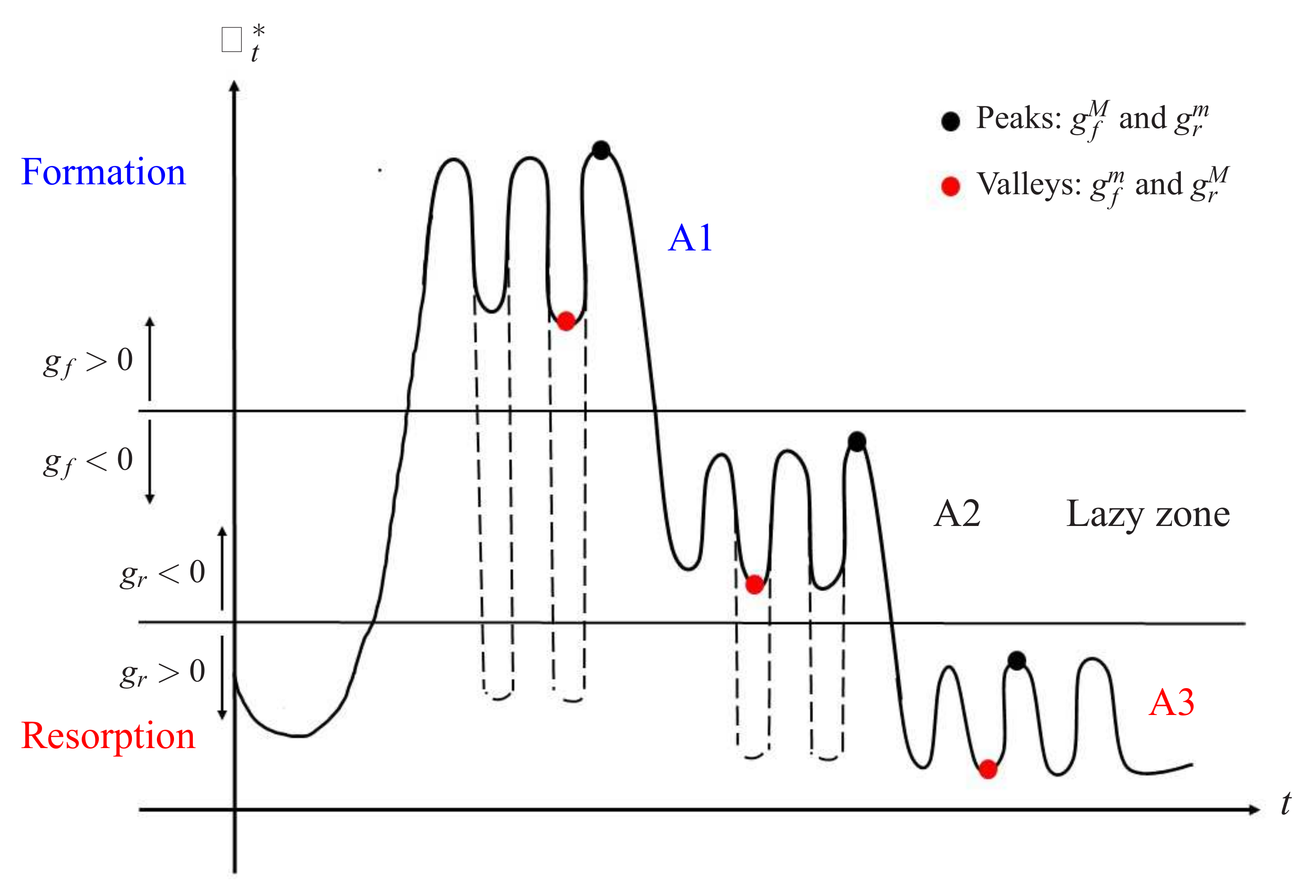
As stated by Carter et al. [
35], bone remodelling depends on the maximum stresses that the bone withstands throughout its load history. Thus, the peaks of mechanical stimulus reached in time-varying loads would control the bone remodelling response, and it is important to note that these peaks can be reached at different instants at each bone site. Let us consider, for example, the temporal evolution of the mechanical stimulus shown in
Figure 5, with three different activities. The remodelling response is assumed to depend on the maximum stimulus representative of each activity (black dots in
Figure 5). The cycles are grouped by the level of stimulus and an average cycle must be chosen as representative of a certain activity. In
Figure 5, A1, A2 and A3 represent, respectively, a high, medium and low intensity load. The mechanical stimulus must be obtained by superimposing the effect of all activities [
35], but let us consider for a moment that only one of those loads is applied. In such case, A1 would stimulate formation, A3 resorption and A2 would produce no net change of bone mass.
The peaks of the stimulus coincide with the maximum of the formation criterion function,
, which is proportional to the stimulus. Those peaks are termed here,
. Since the resorption criterion function,
, is inversely proportional to the stimulus [
4], the local minimum of this function,
, also coincides with the peaks of the stimulus (it must be noted that
and
do not necessarily coincide. They are simply reached at the same instant). Analogously, the valleys of the stimulus coincide with the minimum of
and the maximum of
, termed here
and
, respectively (red dots in
Figure 5).
The procedure to analyse the bone remodelling process for time-varying loads begins with the calculation of the stimulus (and thus, of
and
) at every point of the FE mesh throughout the cycle, in order to capture the peaks
and
for each element. Based on the ideas of Carter et al. [
35], Ojeda assumed that only the peaks are important from the bone remodelling perspective. Therefore, the activities plotted in solid and dashed lines in
Figure 5 would lead to the same bone remodelling response, regardless of the valleys. The criterion must identify the peaks and place them in one of the three regions: formation, resorption or lazy zone. Thus, the remodelling criteria (
14) are replaced by:
It is important to highlight that and are not necessarily reached at the same instant for all the elements. This is the reason why a detailed description of the cycle is required in the modification proposed by Ojeda, as the remodelling response at each element could be driven by the stress-state reached at a different time point. For the same reason, the simplification consisting in considering three instants of the cycle as independent loads is not valid.
2.7. FE Simulation of the Gait Cycle—Temporal Evolution of Stresses and Strains in the Femur
The temporal evolution of stresses and strains in the femur during the gait cycle can be obtained by solving an elastic problem. Let be an open bounded domain and be its boundary, assumed to be Lipschitz continuous and divided into two disjoint parts and where Dirichlet and Neumann boundary conditions are applied, respectively. We denote, by , a generic point of and as the outward unit normal vector to at a point . The Einstein summation notation was adopted and a Cartesian basis () can be used without loss of generality.
Let , and denote the displacement field, the stress tensor and the linearised strain tensor, respectively. () represents the Cartesian tensorial basis. Let denote the known vector of body forces, the known vector of surface traction forces at and the known displacements at .
The Momentum Conservation Principle states:
where
denotes the partial derivative
and
denotes the second derivative with respect to time. The right-hand side of Equation (
22) represents the inertial force per unit volume. Linearised strains are related to displacements by:
and finally, strains and stresses are related by the constitutive equation, which for linear elastic materials reads:
where
are the components of the fourth-rank stiffness tensor
. In the case of an isotropic material, this tensor is completely defined by the Young’s modulus,
E, and the Poisson’s ratio,
, which are expressed as the functions of the density in the case of bone (see Equation (5)). In general anisotropic materials, this tensor has 21 independent elastic constants. In our anisotropic case, bone is assumed to be an orthotropic material, and the compliance tensor (inverse of the stiffness tensor) is given as a function of the fabric tensor (recall Equation (
10)). The elastic problem is completed with the Dirichlet and Neumann boundary conditions, respectively, applied at
and
:
This boundary value problem rarely has an analytical solution, and hence, it is usually solved by means of the FEM, as carried out here.
At this point, the FE model of the femur had a complete definition of density, and consequently, of stiffness. Next, the muscle loads and joint reaction forces, estimated in the gait analysis, were applied as external forces. Muscle loads were applied as concentrated loads at the insertion points and with the direction defined by the insertion and origin points (taken from OpenSim [
22]). The joint reaction forces were applied as concentrated loads on the corresponding articular surfaces, i.e., the hip reaction force on the surface of the femoral head and the knee reaction force on the surface of the epicondyles or of the epicondylar fossa. In both cases, the node of application at each instant was calculated as follows: A line was defined as passing through the corresponding joint centre (defined in OpenSim [
22]) and with the direction of the reaction force at that instant. The reaction force was applied at the node closest to the intersection of the articular surface with that line. Furthermore, the minimum number of displacement boundary conditions (isostatic) was applied to restrain the rigid body motion of the FE model. The loads were varied over time, as a result from the gait analysis, but a quasi-static analysis was performed by disregarding the inertial forces in the FE simulation (
in Equation (
22)). Nonetheless, we must note that the loads estimated with OpenSim arise from enforcing the equilibrium of all the external forces, including the inertial ones. For that reason, these inertial forces were indirectly considered in the simulations. The FE model, including the loads and the boundary conditions, is provided in the
Supplementary Materials.
This pseudo-static analysis provided the temporal evolution of stresses and strains at each element
e of the mesh (in fact, it is obtained at each integration point in full integration elements. In our case, C3D4 elements have only one integration point, which can be, therefore, identified with the element. In the case of C3D10 elements, the variables were evaluated at the centroid of the element) and at every instant
i of the gait cycle. Several variables were derived from the stress and strain tensors (see
Section 2.9). For a certain variable proposed as stimulus
S, its value was calculated at each instant
i and for each element,
e, thus, yielding
. Then, the following maximum, minimum and amplitude were defined to represent its evolution throughout the gait cycle:
Note that the definition of
is related to the aforementioned hypothesis of Carter, according to which the local remodelling response would depend on the peak of stress that a bone site withstands throughout its load history [
35]. As stated before, the peaks of stress do not necessarily occur at the same time for all bone sites. Therefore, considering only the loads of a single instant of the cycle is not enough to analyse the remodelling response of the whole bone. Even considering three instants of the cycle, as carried out in [
4,
6], is not enough. A detailed description of the gait cycle is required and the modification of the BRM presented in
Section 2.6 is related to this idea. The variable,
, generalises this concept of the peak of stress to the peak of stimulus. As an alternative to the maximum of the stimulus throughout the cycle, the amplitude is considered in
.
2.8. Correlation Coefficients
The Spearman and Pearson correlation coefficients were used to assess the statistical dependence between the bone density and the variables defined later in
Section 2.9. Based on the definitions made in Equation (26), the following coefficients were calculated, taking each element as a point of the sample:
R, between the maximum throughout the cycle and the apparent density .
R, between the amplitude throughout the cycle and the apparent density .
where
j stands for
P (Pearson) or
S (Spearman). Weighted coefficients were calculated to account for the relative importance of a sample point based on the volume of the element. The expressions of the weighted correlation coefficients are given in
Appendix A. The Spearman correlation coefficient is a non-parametric measure of rank correlation and it assesses how well the relationship between two variables can be described by a monotonic function. In particular, it evaluates if there is a concordance between the highest density and the highest values of a predictor variable. The Pearson coefficient is a parametric measure of correlation between two variables that assesses if they are related by a specific function. In particular, the linear, quadratic and power correlation coefficients were calculated for those variables that yielded a high Spearman coefficient, in order to confirm a strong correlation and to evaluate the best function relating the variable to bone density. Despite that strain energy density (SED) did not yield a high Spearman coefficient, it was also correlated with bone density through the Pearson coefficient and using those three functions, for reasons that will be explained later.
It is important to note that concentrated loads or displacement boundary conditions can produce spurious stress concentrations in the FE model. For this reason, the elements closest to the nodes where loads or displacement boundary conditions were applied up to a distance of two elements in all directions were removed from the correlations.
2.9. Evolution of Stresses and Strains—Definition of Predictor Variables
The set of predictor variables analysed in this work includes some variables that measure the magnitude of the stress or the strain tensor and the SED that accounts for the magnitude of both tensors in a single variable. The principal stresses are named here,
, and analogously,
. The maximum and minimum principal stresses (
,
) and strains (
,
) are proposed as predictor variables. The maximum tensile stress is defined as:
and the maximum compressive stress as:
The fluctuations of stresses throughout the cycle can be measured by the variable:
where the superscripts
M and
m follow the definition given in Equation (26). The absolute maximum principal stress (AMP
) and strain (AMP
) are defined analogously as:
The von Mises (
) and Tresca (
) stresses (in metallic materials, these variables are used in yielding criteria, which are not applicable to bone, but they can be regarded as well as a measure of the stress intensity) as well as the hydrostatic stress (
) and volumetric strain (
) are also proposed as predictor variables:
Finally, the SED, which has been extensively used as a mechanical stimulus in bone remodelling algorithms, is also proposed as a predictor. SED is given by the following expression in terms of the stress (
) and strain (
) tensors or their components (
,
):
Beaupré et al. [
3] defined the mechanical stimulus that drives bone remodelling,
, as a combination of two factors: the SED and the number of cycles of each activity. Furthermore, these authors proposed to superimpose the effect of all the activities,
i, performed by the individual during one day, by weighting the SED of each activity, SED
, with the corresponding number of cycles, n
. The interested reader can consult the details in [
3]. In the following, we will assume that only the most representative activity is carried out daily and that the number of cycles is constant. In that case, there is a linear relationship between
and SED [
3]:
In other words, we can identify
and SED for correlation purposes. More importantly, Beaupré et al. proposed to take into account the porosity of the tissue to redefine the mechanical stimulus. Thus,
represents the mechanical stimulus at the continuum (or macroscopic) level. SED can be calculated through FEM and if the constant
k in Equation (
33) is known, the mechanical stimulus at the continuum level,
, can also be evaluated for each element of the mesh. Beaupré et al. hypothesized that this mechanical stimulus must be sensed by the existing tissue within the element in order to produce a remodelling response. Therefore,
can be distributed among the tissue existing in the element through porosity, analogously to what localisation procedures do in multiscale approaches, i.e., allowing to move from the macro to the micro scale. To this end, those authors proposed the following mechanical stimulus at the tissue (or microscopic) level [
3]:
where
is the porosity and
n = 2 is the exponent they used [
3]. In this way, if the porosity of one element is close to 1, the mechanical stimulus must be distributed among the little existing tissue and this will be heavily overloaded. Later, we will analyse the effect of the exponent
n. As stated before, the linear, quadratic and power Pearson coefficients were also evaluated for the SED. The rationale for this is based on the theoretical dependence of SED upon density, which can be deduced from previous works found in the literature [
2,
35]. In the particular case of a uniaxial stress-state, the stress tensor is
, with
being the loading direction and
the applied stress. In such case, and assuming a linearly elastic and isotropic behaviour for bone, the SED can be calculated through Equation (
32) as:
where
is the strain tensor and
is the strain in the loading direction. The asterisk has been added to highlight that this expression corresponds to a particular case. Additionally, a typical power correlation between the Young’s modulus and the apparent bone density can be assumed, for example Equations (5a) and (
7), which would read:
where
B and
are constants. In this case,
can be rewritten using Equations (
33) and (
35) as:
where the constants preceding the factor
were grouped in a new constant
K. The right-hand side of Equation (
37) is only valid if bone is subjected to a constant strain, which would be in accordance with the Mechanostat Theory. Under all these assumptions,
could be related to the bone apparent density through a power law. Recalling Equation (
34) and given that
is equal to the bone volume fraction, which is proportional to the bone density, the mechanical stimulus at the tissue level,
, could also be related to bone density through a power law. For this reason, we will check if such a power correlation between apparent density and
(or equivalently SED) or
is suitable.
3. Results
The weighted Spearman correlation coefficients between bone density and the predictors proposed here are shown in
Table 1 for the constitutive model
AnisoH. As stated before, three different values were used for the grey level threshold (GLT) used in Equation (
4), thus, leading to three different FE models (see
Figure 2). The correlation coefficients are given in the three cases for comparison.
The fact that the Spearman correlation coefficient is non-parametric makes it more appropriate to evaluate the correlation between density and the variables, as it implies no assumption on the type of relationship. It simply establishes if there is a concordance between those points having the highest density and those having the highest values of a certain predictor.
It can be seen that most of the stress magnitudes are highly correlated with the density except for the peak of the minimum principal stress, , for obvious reasons, as the sign of (usually negative) is considered in the calculus of this peak. Therefore, usually corresponds to the lowest absolute value throughout the cycle. The amplitude, , is better correlated with the density as it usually measures the range of the compressive stress.
The strain magnitudes are poorly correlated with the density, in some cases with negative coefficients. SED (or ) is only moderately correlated with the density and not correlated at all if it is corrected to account for the porosity ().
Regarding the influence of GLT, it can be seen that though the values of R are different, the same trend is observed in the three cases. In fact, if we ordered the predictors based on R, the same order would result for the three GLT.
The weighted Pearson correlation coefficients are shown in
Table 2 for the constitutive model,
AnisoH. Only some of the variables previously analysed in
Table 1—those that are considered more interesting—are studied here; in particular, some of the stress variables that had a higher Spearman coefficient together with the SED at the continuum and at the tissue level for n = 1 and n = 2 (see Equation (
34)). The Pearson coefficients are parametric and presuppose a certain relationship between the variables being correlated. Thus, we have tried linear, quadratic and power functions (see
Appendix A for details).
Compared to the Spearman, the Pearson correlations have worsened notably as we are forcing them to fit a certain function which is probably not the most appropriate to relate the density with the predictor. Among the three types of functions tested, the quadratic is slightly better, followed by the power and the linear function. The low correlation between SED and density stands out—something that does not improve in the case of SED at the tissue level—for which even negative correlation coefficients were obtained, as in the case of the Spearman coefficients.
Table 3 and
Table 4 compare, respectively, the Spearman and Pearson coefficients obtained using the three constitutive models analysed in this work:
AnisoH,
IsoH and
IsoJ. As indicated above, the effect of GLT was not important, and hence, only one case (GLT = 80) was studied. It can be noted that the effect of the constitutive model is negligible on the Spearman correlations and small on the Pearson correlations, at least for the three cases tested here. The biggest difference is obtained for the power fit between the
IsoH and
IsoJ models, which, in turn, follow a different power correlation between the density and the Young’s modulus, but is not greater than 0.03.
We have also analysed the spatial distribution of the correlations, in particular of the Pearson coefficients (power fit), by assessing separately the correlations for the elements of the proximal, distal and diaphyseal thirds (see
Table 5). The aim of this comparison was to investigate if there are regions of the femur where the density is better to the predictors. Given the limited influence of GLT and the constitutive model, we only show the case GLT = 80 and
IsoH. Besides, we only compare some of the variables that show a higher correlation (
, AMP
) and only the coefficients for the maximum variable throughout the cycle, R
. The other stress variables follow the same trend, as well as R
. The comparison of the strain variables is meaningless since they are not correlated with density, as shown previously. It can be noted that the correlation coefficients are high in the diaphysis, significantly worse in the proximal and especially worse in the distal third, influenced by the simplified way the joint reaction forces were modelled. They were applied as concentrated nodal forces, as explained in
Section 2.7, rather than as a load distributed over the articular surface, as it actually occurs. This simplification affects the stresses near the articular region and, therefore, the correlations. The hip joint force can be more plausibly applied as a concentrated nodal force since the pressure on that joint spans a narrower region than that on the knee joint. Probably, this makes the correlations be slightly better in the proximal third than in the distal one.
The influence of the mesh (C3D4 vs. C3D10) was analysed by comparing the correlation coefficients in
Table 6; in particular, the Spearman and the power Pearson coefficients in the case GLT = 80 and using the constitutive model
IsoH. The Pearson coefficients improved moderately with the use of quadratic elements (C3D10), but only for the good predictors, i.e., those variables that are highly correlated with density. The rest of variables, such as
and the strain magnitudes (not shown), did not improve their correlations. The other types of fit (linear and quadratic) also improved with C3D10, although to a lesser extent. It is noteworthy that the Spearman coefficients were almost identical in both meshes.
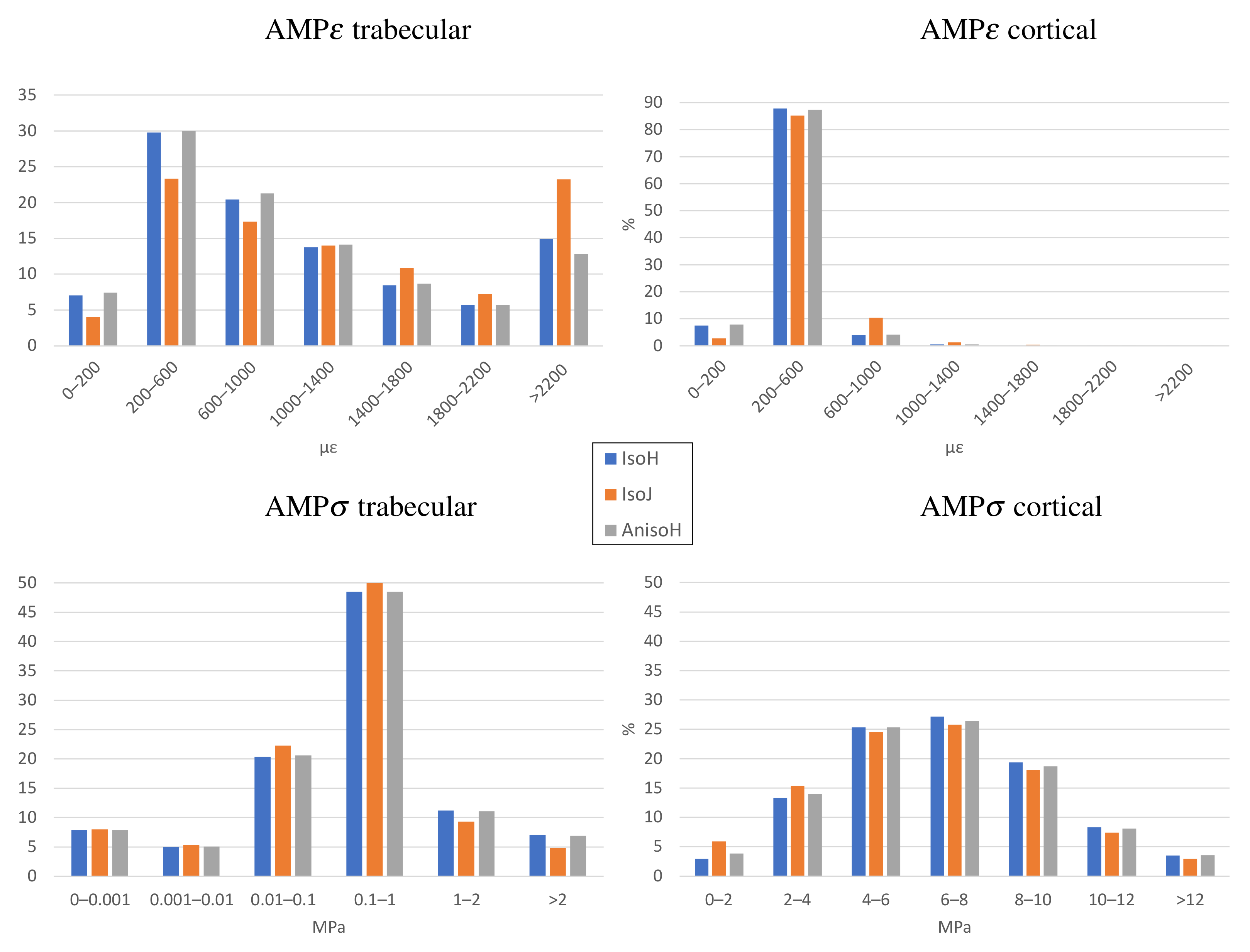
Histograms
There are so many points involved in the correlations that the plots of density against the different variables are very difficult to distinguish. Instead, histograms are used to show the percentage of volume occupied by those elements whose values of AMP
or AMP
are within a given range. The elements of cortical (
g/cm
) and trabecular bone (
g/cm
) have been separated into two different histograms and the results for the three constitutive models were plotted jointly (see
Figure 6). Thus, for example, in the model
AnisoH, the elements of trabecular bone whose AMP
is in the range [200,600]
occupy 30% of the total volume of trabecular bone (
g/cm
).
It can be seen that while the strain range is similar for cortical and trabecular bone, the stresses are completely different, with trabecular bone having stresses several orders of magnitude lower than cortical bone. In general, strains are found in a very narrow range, especially in the cortical bone, for which 87% of the volume has AMP
in the range of 200–600
. This is not so evident in trabecular bone, though 51% is still within the range of 200–1000
and 65% is in the range of 200–1400
. This is still a narrow range, as overload strains are up to 4000
[
36,
37].
4. Discussion
A linear function (Equation (
3)) was used here to estimate the bone apparent density from the grey level of the CT scan [
23,
24,
25,
26]. As in these previous works, the CT scan could not be calibrated, and thus, a threshold was set by identifying the grey level of the diaphyseal canal with bone marrow, that is, with null bone density. Notwithstanding, the greyscale value inside the canal was found to vary in the range of 70–90 and, thus, three different grey level thresholds (GLT) were used and their effect was investigated. The same trend was observed in R for the three values of GLT. Therefore, we can state that the choice of GLT had no effect on the correlation coefficients (see
Table 1 and
Table 2), and hence, on the overall conclusions of this study. For that reason, the rest of results were compared only for the intermediate GLT = 80.
In general, the variables derived from the strain tensor has a low correlation with density and this can be due to the fact that the strains are concentrated in a narrow range, as deduced from the histograms. On the contrary, the stress-related variables are distributed over a much wider range and they are very closely related to density as the correlation coefficients showed. The high correlation found between density and the von Mises, Tresca, absolute maximum principal stress (AMP) and the fluctuation of stresses () are noteworthy.
On the other hand, SED is only modestly correlated with density, probably because it depends on the strains, which are very poorly correlated with . Since SED also depends on the stress level, the histograms of SED (not shown) are as spread as the histograms of stress; however, in view of the correlations, its variation does not seem to be as coupled to density as the mere variation of stress is. However, if SED seems a modest predictor of density, the mechanical stimulus at the tissue level proposed by Beaupré () is even worse, as it yields negative correlation coefficients.
The Spearman coefficient is probably the most simple indicator that two variables are correlated by a monotonic function, since it does not assume any specific relationship as does the Pearson coefficient. If R is positive and high for a certain variable, this means that density increases with that variable, and that a large part of that increase can be explained by the variable, without assessing what specific relationship exists. Hence, that variable can serve as a good predictor of density in a bone remodelling model, though the particular relationship between the density and the specific variable should be further investigated. In this regard, the linear, quadratic or power functions tried for the Pearson coefficients worked only moderately well. Only and AMP showed a value of R slightly over 0.8 (up to 0.861 for in the IsoJ model). This means that R 0.64, i.e., around 64% of the variation of the density, can be explained by (up to 74% in the IsoJ model).
Only some of the variables appearing in
Table 1 were chosen for assessing its Pearson coefficient, those having a high Spearman coefficient plus SED and its related variables (
), for its common use as a mechanical stimulus in many models of bone remodelling. Obviously, if the Spearman coefficients of SED and its related variables were low, the respective Pearson coefficients could not improve them, but it is worth noting the very low values of R
obtained for SED compared to R
. This would mean that Equation (
37) was not very appropriate, probably because of the many assumptions involved in it, viz: uniaxial stress-state, isotropic material and power correlation between Young’s modulus and density.
The distribution of two variables, one representing the stress-state (AMP
) and one representing the strain-state (AMP
), was analysed by means of histograms (see
Figure 6) that distinguish between cortical (
g/cm
) and trabecular bone (
g/cm
). These histograms showed that the strains are concentrated in a relatively narrow range in the case of trabecular bone. Around 65% of the volume of trabecular bone was found to be within the range AMP
[200–1400]
in the
AnisoH model, 62% in
IsoH and 53% in the
IsoJ. The range was particularly narrow in the case of cortical bone, as about 85% of its total volume was found in the range AMP
[200–600]
for all constitutive models.
It is noteworthy that the range of strains obtained here was low compared with the normal strains indicated by the Mechanostat Theory (between 800 and 1200
[
10]). Nonetheless, other authors have established a different range of normal strains in the so-called “adapted-window” of the Mechanostat, between 200 and 1500
[
36,
37]. Yet, the strains seem relatively low for models,
AnisoH and
IsoH, which are likely overestimating the bone stiffness. The correlation, (5a), used by model
IsoJ, is probably more adequate in view of the strains it produces.
In contrast to strains, the stresses are more uniformly distributed and over a much wider range, with the stresses of trabecular bone being one or two orders of magnitude lower than those of cortical bone. This strong relationship between bone density and stress is confirmed by the high Spearman correlation coefficients of most stress variables (see
Table 1).
The distributions and correlations of strain and stress variables would confirm that bone is adapted to withstand a constant strain, or at least a strain within a narrow range, in accordance with the Mechanostat Theory, while the local stress-state seems to determine the bone density. This would suggest the use of a strain variable as the mechanical stimulus
S in evolutionary BRM (see Equation (
1)), such that bone density changes if the strain is out of the normal or adapted range. On the contrary, a stress variable would be more appropriate for the stimulus in a non-evolutionary BRM (see Equation (
2)), such that the stress would determine the bone density at a given location. In the case of cyclic loads, such as the one applied here, a variable measuring the fluctuations of stresses throughout the cycle seems the more appropriate mechanical stimulus among those tested here, though the specific relationship between density and stress is yet to be determined. In no case does the SED seem a suitable variable to be used as the mechanical stimulus in BRM.
We have compared three constitutive models (
AnisoH,
IsoH and
IsoJ) in order to check whether the correlation between predictors and density,
, is being forced by the relationship between stiffness and density,
, in particular for those predictors derived from the stress tensor (for the sake of generality, we should write
, with
being the stiffness tensor, in order to account for anisotropic materials. However, the rationale provided is independent of this distinction and we will continue with
). It is well known from the literature that
F is a monotonically increasing function and given that the stiffer elements tend to withstand higher stress levels, we should expect a function such as
to be monotonically increasing as well. Thus, if we write:
we can expect a monotonically increasing function relating
and
, in other words, a positive correlation
for the predictors derived from the stress tensor. Therefore, it could seem that the function
is forcing
and it is so to some extent, especially for the Spearman correlation coefficients. However, if
were the only determinants of the correlation
, this correlation should depend on the constitutive model and it does not—significantly, at least. Indeed, the increase in stiffness from
IsoJ to
IsoH is quite remarkable (up to 70%, see
Figure 3, left) and yet the Pearson correlations do not change much from one model to the other (see
Table 4). Moreover, since the ratio of stiffness is non-uniform (see
Figure 3, right), a redistribution of stresses could be expected that would cause the stress patterns of the two models not to coincide. The same could be said of the comparison between models
AnisoH and
IsoH. Such redistribution of stresses would, therefore, affect the Spearman correlation coefficients or the AMP
histograms, but both are almost identical for the three models (see
Table 3 and
Figure 6). Hence, we can conclude that the assumed constitutive model has no significant effect on the correlations.
However, there is another argument to support that
is not completely forced by the constitutive behaviour, but only to some extent. Certainly, Equation (
38) is incomplete as the stress-state also depends on the loads and boundary conditions:
where
stands for the set of loads applied to the domain, including the body forces, the surface tractions applied on the boundaries (i.e., Neumann boundary conditions) and the reaction forces (and consequently the Dirichlet boundary conditions). Apart from that, the predictors,
S, are obtained as a function of the stress tensor, that we can denote as
, thus leading to:
In view of Equation (
40) the predictors,
S, need not be predetermined only by the function
, not even the Spearman correlation coefficients, as the function
G is not necessarily monotonic. This is confirmed by the different Spearman coefficients obtained for different predictors (see
Table 1 and
Table 3). It should be noted that the same concepts that are behind the
G functions can be applied to the predictors derived from the strain tensor or the SED-based predictors.
An example can serve to illustrate the key role played by the loads on the correlations
. We have obtained these correlations for every instant of the gait cycle separately. The stress and strain tensors obtained at each instant
i were used to assess
(recall
Section 2.7) and these variables were correlated with
to give R
, a weighted Pearson correlation coefficient for each instant
i. The worst coefficient between AMP
and density throughout the cycle was R
= 0.48 (for the quadratic fit and in the case GLT = 80, constitutive model
IsoH and C3D4 elements), which is far from R
= 0.804. The former is a very poor correlation. (R
= 0.23, i.e., only about 25% of the variance of density can be explained by AMP
and this is probably because the loads at that instant are not representative of the gait cycle. In fact, the loads at a single instant cannot be representative of the entire cycle on a general basis.
In summary, the function is contributing to obtain the correlations , at least for stress-based predictors, but only to some extent. There are other factors, not influenced by that function, that play an important role in the correlations; an accurate estimation of the loads is crucial, taking into account the variation of stresses throughout the cycle is also important and an appropriate choice of S (funtion G) is key to predicting density.
The type of element (C3D4 vs. C3D10) had a relative importance on the results, as the linear elements (C3D4) are stiffer than the quadratic ones (C3D10). The latter yielded moderately higher stresses and strains, which were slightly better correlated with density through a power law than those obtained with C3D4 elements (see
Table 6). The linear and quadratic fits (not shown) also improved with C3D10, but to a lesser extent. Notwithstanding, the C3D4 mesh had a sufficient element density and was accurate enough as evidenced by the fact that the stress and strain patterns are almost identical in both meshes. Consequently, the Spearman correlation coefficients derived from both are also almost identical. For that reason, the use of C3D4 elements was justified, at least for the mesh density employed in our model.
Among the limitations of this study we must note that only one activity (walking) has been considered, among the many activities that a person can carry out in a normal day. Other activities can load the femur in a different way than walking, thus, affecting the local bone density. This could partially explain the variance of density not explained by our correlations. However, walking is by far the most common activity affecting the lower limb and the most common activity performed by the subject under study. Hence, little influence of other activities can be expected.
The joint loads were applied in a simplified way, as nodal-concentrated loads instead of loads distributed over the articular surface. This approximation is especially significant in the knee reaction force and this could explain the lower correlation coefficients found in the distal third of the femur. Another limitation is that the CT scan could not be calibrated, but we have shown that this fact did not influence the conclusions drawn. Finally, it must be noted that only one individual, a male healthy subject, was studied. As future work, it would be interesting to repeat the study in other cases, including different bones, age, gender, health status, bone pathologies, etc., in order to confirm whether these variables or others alter the dependence of bone density on the proposed predictors.

 ,
, 


