Optimal Selection of Conductor Sizes in Three-Phase Asymmetric Distribution Networks Considering Optimal Phase-Balancing: An Application of the Salp Swarm Algorithm

Abstract

This paper presents a new methodology to simultaneously solve the optimal conductor selection and optimal phase-balancing problems in unbalanced three-phase distribution systems. Both problems were represented by means of a mathematical model known as the Mixed-Integer Nonlinear Programming (MINLP) model, and the objective function was the minimization of the total annual operating costs. The latter included the costs associated with energy losses, investment in conductors per network segment, and phase reconfiguration at each node in the system. To solve the problem addressed in this study, a master–slave methodology was implemented. The master stage employs a discrete version of the Salp Swarm Algorithm (SSA) to determine the set of conductors to be installed in each line, as well as the set of connections per phase at each of the nodes that compose the system. Afterward, the slave stage uses the three-phase version of the backward/forward sweep power flow method to determine the value of the fitness function of each individual provided by the master stage. Compared to those of the Hurricane-based Optimization Algorithm (HOA) and the Sine Cosine Algorithm (SCA), the numerical results obtained by the proposed solution methodology in the IEEE 8- and 25-node test systems demonstrate its applicability and effectiveness. All the numerical validations were performed in MATLAB.

1. Introduction

Due to the rapid growth of the world population, the global demand for electricity has increased, leading to a complete reliance on electrical systems to meet all basic human needs [1,2]. As a result, electrical networks that include hybrid systems, renewable energies, and three-phase distribution systems have become essential because they ensure that (industrial, commercial, and residential) end users have access to the amount of energy they need, when they need it, and at a reasonable cost [3,4,5].

An important characteristic of electrical distribution systems is that they have a radial topology, which means that there is a single path from the main node (substation) to the rest of the nodes that make up the network [6]. This type of network topology considerably reduces the costs associated with distribution lines and protective devices. In addition, three-phase distribution systems operate in an unbalanced fashion for two reasons: (i) the impossibility of applying the transposition criterion due to the short length of the distribution lines (tens of kilometers), which causes asymmetries in the network segments [7]; and (ii) the presence of single-phase, two-phase, or three-phase loads, with three-phase loads being connected either in a star (Y) or triangle ($\Delta$) configuration, which causes intrinsic imbalances in the currents flowing through the lines and the nodal voltages [8,9].

These intrinsic imbalances, added to the radial topology of three-phase distribution systems, significantly increase their power losses and thus result in higher electricity bills for end users [10]. In Colombia, the Energy and Gas Regulation Commission (CREG, for its acronym in Spanish) allows a maximum of 8% of power losses to be charged to end users, which is reflected in their final bill [10]. Hence, if power distribution companies reduced the amount of power losses to less than 8%, they could earn the surplus through billing. If power losses, however, exceed that percentage, network operators cannot charge users more than it is allowed by the CREG and would miss potential financial gains as a result of the operational inefficiencies of their networks [11].

It is clear from the above that the intrinsic characteristics of three-phase distribution networks can cause negative effects not only in terms of technical aspects (such as power losses, voltage profiles, and the loadability of lines) but also in financial terms. This, indeed, poses a challenge for engineers in charge of designing, planning, and operating three-phase distribution networks, as they must devise effective strategies and methodologies to optimize and expand them. An effective methodology should guarantee the financial viability of the network operator over a given time horizon and the safe and reliable provision of the service required by end users, while meeting the quality standards set forth by the governmental entities in charge of regulating the electricity service [12].

Given the importance of strategies for planning and operating power distribution networks, various approaches have been proposed, including (i) optimal conductor size selection [13] and (ii) optimal phase-balancing [10]. The optimal conductor size selection problem in distribution networks is a classical problem in terms of network expansion that has been extensively studied in the specialized literature. It is characterized by its nonlinear and non-convex nature, which makes it challenging to solve [14]. The phase-balancing problem has been thoroughly explored in the specialized literature as well, despite being highly complex due, also, to its nonlinear and non-convex nature [15]. However, it has caught the attention of researchers because it is a low-cost solution that guarantees correct system operation and reduces power losses in three-phase distribution networks by up to 24% [10].

According to the most recent studies in the field, the optimal conductor size selection problem is often solved using combinatorial optimization strategies based on master–slave methodologies [16]. For instance, in [17], the authors presented a master-slave methodology that combines the tabu search algorithm and the backward/forward sweep power flow method. The objective function they employed was the minimization of the costs associated with investment in conductors and power losses during a year of operation under two operating scenarios: (i) a peak demand during the entire year of operation and (ii) a demand curve discretized into three periods. In all the simulations, the authors considered a balanced three-phase distribution network, i.e., the equivalent of a single-phase network. To demonstrate the applicability and efficiency of the proposed solution methodology, they used the 8- and 101-node test systems. However, they did not perform a statistical analysis to evaluate the repeatability of the proposed methodology, analyze processing times, or compare said methodology with other optimization techniques to validate their findings.

In [18], the whale optimization algorithm was employed to solve the optimal conductor selection problem in the single-phase equivalents of the 16- and 85-node radial distribution systems. The objective function in that study was the reduction of the overall energy costs and the investment in conductors over a five-year period, considering a peak demand during the entire planning horizon. When compared to two other optimization techniques reported in the specialized literature, this solution methodology demonstrated its efficiency. The authors, however, did not conduct a statistical analysis or evaluate processing times in order to validate the repeatability and robustness of their proposed solution algorithm.

In [19], the authors proposed using the branch wise minimization technique to solve the optimal conductor selection problem. Their objective function was the minimization of the costs associated with the main feeder and energy losses during a year of operation in balanced three-phase distribution systems. The results obtained in the 16-node test system demonstrated the applicability of the proposed solution methodology. However, they did not compare said methodology with other metaheuristic techniques, making it difficult to assess its performance in terms of repeatability and processing times.

In [20], the evaporation rate water cycle algorithm was used to select the best set of conductors for the single-phase equivalent of the 16-node radial distribution system. The main goal in such study was to reduce the costs of investment and those associated with energy losses. According to the results, the proposed methodology was able to find an optimal solution while respecting the voltage and current constraints defined in the mathematical model of the problem. In addition, the authors compared their proposed methodology with another metaheuristic technique reported in the literature. However, they did not conduct a statistical analysis or evaluate processing times, which makes it difficult to evaluate the repeatability of their proposed algorithm.

In [21], the authors addressed the optimal conductor selection problem in distribution networks with a radial topology, assuming that they were balanced three-phase systems. To solve such problem, they employed the tabu search algorithm, and the objective function was the minimization of the costs of investment and those associated with energy losses for a discretized demand curve under three different load scenarios. In addition, they used the 9- and 25-node test systems to demonstrate the applicability and efficiency of their proposed methodology and compared its results with those of the sine cosine algorithm to evaluate its performance in terms of repeatability and processing times.

Since all the optimization methodologies mentioned above assume that the distribution networks are balanced three-phase systems, a single-phase equivalent is employed to solve the problem under analysis. This assumption, nonetheless, does not allow us to consider all the phenomena that occur in real distribution systems (i.e., unbalanced three-phase systems [22]). As a result of this, the authors of [13] presented a master–slave methodology to optimally select conductors for three-phase distribution networks with unbalanced loads. To that end, they used the vortex search algorithm, along with the backward/forward sweep power flow method in its three-phase version. The objective function they considered was the minimization of the investment costs together with the costs associated with the energy losses in the system over a year of operation under three demand scenarios. In the first scenario, the demand consumes the maximum power during the entire study period. In the second scenario, a demand curve discretized into three different load conditions is used. Finally, in the third scenario, a typical demand curve is considered—this is the scenario that best represents the real behavior of users. To demonstrate the applicability and efficiency of their proposed methodology, the authors employed the 8- and 27-node test systems and used, for comparison purposes, the Traditional Genetic Algorithm (TGA), the Chu & Beasley Genetic Algorithm (CBGA), and the Tabu Search Algorithm (TSA). However, they did not perform a statistical analysis or evaluate processing times to assess the repeatability and robustness of their proposed solution algorithm. Also, when they developed the mathematical model of the backward/forward sweep power flow method, they failed to consider the asymmetry of the distribution lines.

In order to further illustrate the literature on the matter, Table 1 summarizes the main methodologies that have been employed to solve the optimal conductor selection problem in distribution networks.

Recent studies in the specialized literature have aimed to solve the phase-balancing problem, which is often solved using combinatorial optimization strategies based on master–slave methodologies. For instance, the authors of [10] proposed using the vortex search algorithm to solve the phase-balancing problem in three-phase distribution systems with a radial topology. The objective function they considered was the reduction of power losses in a given demand scenario. They employed the 8-, 25-, and 37-node test systems to demonstrate the applicability and efficiency of their proposed methodology and compared its results with those obtained by the CBGA. In addition, they performed a statistical analysis and evaluated processing times in order to assess the repeatability of their methodology.

Similarly, in [23], the authors used an updated version of the crow search algorithm to solve the phase-balancing problem in the 8-, 25-, and 37-node test systems. Their objective function was the minimization of the total power losses in a given demand scenario. To demonstrate the applicability and efficiency of the proposed solution methodology, they compared its results with those of other metaheuristic techniques reported in the literature. They also conducted a statistical analysis and evaluated processing times in order to assess the repeatability and robustness of their proposed solution algorithm. In [24], the authors solved the optimal phase-balancing problem in three-phase distribution networks with a radial topology using the hurricane-based optimization algorithm. The objective function they considered was the reduction in total power losses. They implemented the 8-, 25-, and 37-node test systems to demonstrate the applicability and efficiency of their proposed methodology and compared it with the vortex search algorithm and the CBGA in order to evaluate its performance in terms of repeatability and processing times.

In [25], the authors solved the phase-balancing problem in unbalanced three-phase distribution systems using a master–slave methodology. In the master stage, an improved version of the CBGA was employed together with the three-phase version of the successive approximation method to estimate the costs associated with energy losses over a year of operation. To determine the value of the objective function, they used daily active and reactive power demand curves. In addition, to validate the results obtained by their proposed solution methodology in the 15- and 37-node test systems and demonstrate its effectiveness, they compared it with some metaheuristic algorithms reported in the specialized literature (e.g., the original version of the CBGA, the vortex search algorithm, the sine cosine algorithm, and the black hole algorithm). They also conducted a statistical analysis and evaluated processing times to determine the repeatability and robustness of their proposed methodology.

Finally, in [26], the authors employed an enhanced version of the sine cosine algorithm to determine the set of load connections per phase in the nodes that make up the 15- and 37-node distribution systems, which are unbalanced systems with a radial topology. Their objective function was the reduction of the annual costs of energy losses (considering typical active and reactive power demand curves) and the costs of swapping the phases of a node (by a work crew). The results obtained by the proposed solution methodology demonstrated its applicability and efficiency and were compared with those of other metaheuristic techniques reported in the specialized literature. Furthermore, the authors performed a statistical analysis and evaluated processing times, which allowed them to determine the repeatability and robustness of their proposed solution algorithm.

Table 1 presents a complete list of the algorithms that have been used in the literature to solve the phase-balancing problem in unbalanced three-phase distribution systems.

The studies listed in Table 1 have the following main characteristics: (i) for the optimal conductor selection problem, they do not consider the unbalanced nature of real distribution systems; (ii) most of the proposed scenarios are far from reality because they do not use typical demand curves; (iii) the methodologies used for both the optimal conductor selection problem and the optimal phase-balancing problem are of a combinatorial nature, which means that they are based on metaheuristic optimization techniques due to the non-convex nature of both problems; (iv) the solution space cannot be exhaustively evaluated in both problems due to their exponential nature, which depends on the number of nodes in the network; and (v) the salp swarm algorithm has not been previously used to solve either of these two optimization problems.

Table 1. Summary of methodologies used in the literature to solve the optimal conductor selection and optimal phase-balancing problems in distribution networks.

	Optimal Conductor Selection
Solution Methodology	Objective Function	Year	Reference
Heuristic index directed method	Minimization of operating costs	2000	[14]
Constructive heuristic algorithm	Minimization of operating costs	2002, 2017	[27,28]
Harmony search algorithm	Minimization of operating costs	2011	[29]
Elitist non-dominated sorting algorithm	Minimization of operating costs	2011	[30]
Particle swarm optimization	Minimization of operating costs	2012	[31]
Genetic algorithm	Minimization of operating costs	2013	[32]
Bacterial search algorithm	Minimization of operating costs	2015	[33]
Imperialism competitive algorithm	Minimization of operating costs	2015	[33]
Sine-cosine optimization algorithm	Minimization of operating costs	2017	[34]
Crow search algorithm	Minimization of operating costs	2017	[35]
Tabu search algorithm	Minimization of operating costs	2018, 2021	[17,21]
Exact MINLP solution	Minimization of operating costs	2018, 2021	[17,36]
Branch wise minimization technique	Minimization of operating costs	2018	[19]
Whale optimization algorithm	Minimization of operating costs	2019	[18]
Evaporation rate water cycle algorithm	Minimization of operating costs	2021	[20]
Vortex search algorithm	Minimization of operating costs	2021	[13]
	Optimal Phase-Balancing
Solution Methodology	Objective Function	Year	Reference
Simulated annealing algorithm	Minimization of power losses	1999	[15]
Genetic algorithm	Minimization of phase unbalance	1999	[37]
Chu & Beasley genetic algorithm	Minimization of power losses	2004, 2012	[10,25,38,39,40]
		2019, 2021, 2021
Ant colony optimization algorithm	Minimization of energy costs	2005	[41]
Particle swarm optimization algorithm	Minimization of phase unbalance	2006, 2018	[42,43]
Immune optimization algorithm	Minimization of operating costs	2008	[44]
Differential evolution algorithm	Minimization of power losses	2012	[45]
Bacterial foraging algorithm	Minimization of power losses	2012	[46]
Vortex search algorithm	Minimization of power losses	2021	[10]
Mixed-integer conic reformulation	Minimization of power losses	2021	[22]
Crow search algorithm	Minimization of power losses	2021	[23]
Sine and cosine algorithm	Minimization of power losses	2021	[26]
Mixed-integer convex approximation	Minimization of average unbalance	2021	[47]
Mixed-integer convex model	Minimization of power losses	2021	[48]
Hurricane-based optimization algorithm	Minimization of power losses	2022	[24]

Table 1. Summary of methodologies used in the literature to solve the optimal conductor selection and optimal phase-balancing problems in distribution networks.

	Optimal Conductor Selection
Solution Methodology	Objective Function	Year	Reference
Heuristic index directed method	Minimization of operating costs	2000	[14]
Constructive heuristic algorithm	Minimization of operating costs	2002, 2017	[27,28]
Harmony search algorithm	Minimization of operating costs	2011	[29]
Elitist non-dominated sorting algorithm	Minimization of operating costs	2011	[30]
Particle swarm optimization	Minimization of operating costs	2012	[31]
Genetic algorithm	Minimization of operating costs	2013	[32]
Bacterial search algorithm	Minimization of operating costs	2015	[33]
Imperialism competitive algorithm	Minimization of operating costs	2015	[33]
Sine-cosine optimization algorithm	Minimization of operating costs	2017	[34]
Crow search algorithm	Minimization of operating costs	2017	[35]
Tabu search algorithm	Minimization of operating costs	2018, 2021	[17,21]
Exact MINLP solution	Minimization of operating costs	2018, 2021	[17,36]
Branch wise minimization technique	Minimization of operating costs	2018	[19]
Whale optimization algorithm	Minimization of operating costs	2019	[18]
Evaporation rate water cycle algorithm	Minimization of operating costs	2021	[20]
Vortex search algorithm	Minimization of operating costs	2021	[13]
	Optimal Phase-Balancing
Solution Methodology	Objective Function	Year	Reference
Simulated annealing algorithm	Minimization of power losses	1999	[15]
Genetic algorithm	Minimization of phase unbalance	1999	[37]
Chu & Beasley genetic algorithm	Minimization of power losses	2004, 2012	[10,25,38,39,40]
		2019, 2021, 2021
Ant colony optimization algorithm	Minimization of energy costs	2005	[41]
Particle swarm optimization algorithm	Minimization of phase unbalance	2006, 2018	[42,43]
Immune optimization algorithm	Minimization of operating costs	2008	[44]
Differential evolution algorithm	Minimization of power losses	2012	[45]
Bacterial foraging algorithm	Minimization of power losses	2012	[46]
Vortex search algorithm	Minimization of power losses	2021	[10]
Mixed-integer conic reformulation	Minimization of power losses	2021	[22]
Crow search algorithm	Minimization of power losses	2021	[23]
Sine and cosine algorithm	Minimization of power losses	2021	[26]
Mixed-integer convex approximation	Minimization of average unbalance	2021	[47]
Mixed-integer convex model	Minimization of power losses	2021	[48]
Hurricane-based optimization algorithm	Minimization of power losses	2022	[24]

Therefore, this paper proposes a master–slave methodology. The master stage uses the Salp Swarm Algorithm (SSA) to simultaneously solve the optimal conductor selection and phase-balancing problems in three-phase distribution systems with a radial topology. The slave stage employs the three-phase version of the backward/forward sweep power flow method to find the value of the objective function. The objective function used in this study is the minimization of the overall operating costs of the distribution system over a one-year planning and operating horizon, which include the costs associated with (i) energy losses, (ii) investment in conductors, and (iii) crew’s intervention at a demand node. Moreover, we consider the asymmetry of the distribution lines (i.e., the electrical configuration of the conductors in the electrical support structures) and the typical active power behavior of an end user. The following are the key contributions of this study to the state of the art:

• A new Mixed-Integer Nonlinear Programming (MINLP) model that represents the optimal conductor selection problem in asymmetric three-phase distribution systems considering an optimal phase-balancing.
• A new master–slave methodology to solve the proposed exact MINLP model. The master stage uses a discrete version of the SSA to define the set of conductors to be installed in all the network segments, as well as the phase connections at all the demand nodes that make up the system. The slave stage employs the three-phase version of the backward/forward sweep power flow method to determine the feasibility of each solution and the operating costs of the network over a year of operation.
• A new master-slave methodology that increases the possibility of finding a global optimum by solving the problem under analysis simultaneously—rather than separately or in stages—thus preventing the algorithm from falling into local optima.

The rest of this paper is structured as follows. Section 2 introduces the mathematical formulation of the optimal conductor selection and phase-balancing problems in unbalanced three-phase distribution systems. In said formulation, the objective function is the minimization of the total annual operating costs. Section 3 describes the proposed master–slave methodology, which combines the SSA and the three-phase version of the backward/forward sweep power flow method. Section 4 presents the main characteristics of the IEEE 8- and 25-node test systems, the overhead line configuration and the typical demand curves used in this study, and the parametric information required to calculate the value of the fitness function. Section 5 discusses the results obtained for the optimal conductor selection and phase-balancing problems and the total annual operating costs. Finally, Section 6 draws the conclusions and outlines future lines of research based on the findings.

2. Mathematical Formulation

The optimal conductor selection and optimal phase-balancing problems in distribution systems are often solved separately by representing them using a MINLP model. In said model, the decision variables are associated with the selection of a type of conductor per phase for each distribution line [13] (optimal conductor selection problem) and with the configuration of phases at each demand node [10] (optimal phase-balancing problem), whereas the nonlinearities of the model appear in the formulation of the three-phase power flow [49]. In this study, however, we propose using a MINLP model to simultaneously solve both problems. In the proposed solution methodology, the objective function is the minimization of the annual operating costs in unbalanced three-phase distribution systems.

The next subsections describe the objective function and the set of constraints that represent the conductor selection and phase-balancing problems considering a dynamic power flow (i.e., including a time-dependent variable).

2.1. Formulation of the Objective Function

The objective function considered in this study includes the costs associated with (i) energy losses over a year of operation, (ii) investment in the conductors to be installed per phase in each distribution line, and (iii) phase reconfiguration at demand nodes. Each component of the objective function is presented in Equations (1)–(4).

$$min{A}_{cost}=f_1+f_2+f_3$$

(1)

$$f_1=C_{kWh}Treal\left(\sum _{h\in \mathcal{H}}\sum _{k\in \mathcal{N}}\sum _{j\in \mathcal{N}}\sum _{f\in \mathcal{F}}\sum _{g\in \mathcal{F}}\sum _{c\in \mathcal{C}}{Y}_{kj}^{fg,*}\left(y_l^c\right)v_{k,h}^f{v}_{j,h}^{g,*}\Delta h\right)$$

(2)

$$f_2=3\left(\sum _{c\in \mathcal{C}}\sum _{l\in \mathcal{L}}{C}_{inv,l}^c{L}_l{y}_l^c\right)$$

(3)

$$f_3=\sum _{k\in \mathcal{N}}{C}_{bal,k}\underset{f\in \mathcal{F}}{max}\left\{\underset{g\in \mathcal{F}}{max}\left\{x_k^{fg}-\left[\begin{array}{ccc}1& 0& 0\\ 0& 1& 0\\ 0& 0& 1\end{array}\right]\right\}\right\}$$

(4)

In these equations, $A_{cost}$ represents the total annual operating costs in the distribution network. $f_1$ is the component of the objective function associated with energy losses over a year of operation. $f_2$ is the component of the objective function that models the investment in the conductors to be installed per phase in each distribution line. $f_3$ is the component of the objective function associated with the costs of reconfiguring the phases at demand nodes. $C_{kWh}$ denotes the average cost of purchasing power at the substation node, while T corresponds to the number of days in a normal year (i.e., 365 days). $v_{k,h}^f$ and $v_{j,h}^g$ represent the complex voltages at nodes k and j for phases f and g at time period h, respectively. $Y_{kj}^{fg}$ is the complex admittance that connects node k in phase f and node j in phase g. $y_{kj}^c$ denotes the binary variable in charge of selecting the type of conductor (c) to be installed in the distribution lines that interconnect node k with node j. Note that $Y_{kj}^{fg}$ is a nonlinear function of the binary variable because the complex admittance value will depend on the type of conductor that is installed per phase in the network segment that connects node k with node j. $\Delta h$ denotes the time period during which the electrical variables are assumed to be constant. $C_{inv,l}^c$ represents the cost of installing a type-c conductor in distribution line l, whereas $L_l$ is the length of the conductor in distribution line l. $C_{bal,k}$ denotes the cost of swapping the phases of a load located at node k. Finally, $x_k^{fg}$ is the binary variable in charge of selecting the type of connection for the loads located at node k. Note that $\mathcal{N}$, $\mathcal{F}$, $\mathcal{C}$, $\mathcal{L}$, and $\mathcal{H}$ are the sets that contain all the nodes, phases, conductor sizes, lines, and time periods, respectively.

2.2. Set of Constraints

The optimal conductor selection and phase-balancing problems in unbalanced three-phase distribution networks encompass a set of constraints that represent multiple operational limitations found in electrical distribution systems, including the complex power balance at each node, voltage regulation limits, the loadability of conductors, and the binary nature of the decision variables [10]. All the constraints that model the problem addressed in this study are defined in Equations (5)–(14).

$$s_{csk,h}^f-\sum _{g\in \mathcal{F}}{x}_k^{fg}{S}_{dk,h}^g=v_{k,h}^f\sum _{j\in \mathcal{N}}\sum _{g\in \mathcal{F}}\sum _{c\in \mathcal{C}}{Y}_{kj}^{fg,*}\left(y_l^c\right)v_{j,h}^{g,*},\left\{\begin{array}{c}\forall f\in \mathcal{F}\\ \forall k\in \mathcal{N}\\ \forall h\in \mathcal{H}\end{array}\right\}$$

(5)

$$i_{l,h}^f=F\left(v_{k,h}^f,v_{j,h}^f,Y_{kj}^{fg},y_l^c\right),\left\{\begin{array}{c}\forall f\in \mathcal{F}\\ \forall l\in \mathcal{L}\\ \forall h\in \mathcal{H}\end{array}\right\}$$

(6)

$$\sum _{g\in \mathcal{F}}{x}_k^{fg}=1,\left\{\begin{array}{c}\forall f\in \mathcal{F}\\ \forall k\in \mathcal{N}\end{array}\right\}$$

(7)

$$\sum _{f\in \mathcal{F}}{x}_k^{fg}=1,\left\{\begin{array}{c}\forall g\in \mathcal{F}\\ \forall k\in \mathcal{N}\end{array}\right\}$$

(8)

$$\sum _{c\in \mathcal{C}}{y}_l^c=1,\left\{\begin{array}{c}\forall l\in \mathcal{L}\end{array}\right\}$$

(9)

$$\sum _{l\in \mathcal{L}}\sum _{c\in \mathcal{C}}{y}_l^c=n-1$$

(10)

$$V_{min}\le \left|v_{k,h}^f\right|\le V_{max},\left\{\begin{array}{c}\forall f\in \mathcal{F}\\ \forall k\in \mathcal{N}\\ \forall h\in \mathcal{H}\end{array}\right\}$$

(11)

$$|i_{l,h}^f|\le \sum _{c\in \mathcal{C}}{y}_l^c{I}_{l,max}^c\left\{\begin{array}{c}\forall l\in \mathcal{L}\\ \forall h\in \mathcal{H}\end{array}\right\}$$

(12)

$$x_k^{fg}\in \left\{0,1\right\},\left\{\begin{array}{c}\forall f\in \mathcal{F}\\ \forall g\in \mathcal{F}\\ \forall k\in \mathcal{N}\end{array}\right\}$$

(13)

$$y_l^c\in \left\{0,1\right\},\left\{\begin{array}{c}\forall c\in \mathcal{C}\\ \forall l\in \mathcal{L}\end{array}\right\}$$

(14)

In these equations, $s_{csk,h}^f$ is the complex power produced by a conventional source at node k in phase f at time period h. $S_{dk,h}^g$ denotes the complex power demanded at node k in phase g at time period h. $i_{l,h}^f$ is the complex current flowing through distribution line l in phase f at time period h. $V_{min}$ and $V_{max}$ denote the voltage regulation limits allowed for all the nodes that make up the network at each time period h. Finally, $I_{l,max}^c$ is the maximum thermal current that a type-c conductor in distribution line l can withstand.

Note that the set of constraints in Equations (5)–(14) has a direct impact on the expected solution to the problem under study because it limits the solution space using physical restrictions associated with the expected operation of the distribution system under steady-state conditions. The following are the most important elements in this formulation:

• The first component in the objective function (i.e., $f_1$) defines the total investment and operating costs of the distribution system plan. Said component is affected by the network’s final voltage profiles, which clearly depend on the conductors selected for each distribution line as well as the final load connection. In addition, the components in the objective function that represent the investment in conductors and the cost balance (i.e., components $f_2$ and $f_3$) are also directly related to the type of conductors selected for each distribution line and the number of interventions required in the distribution network to reduce the load imbalance.
• The power balance constraint defined in Equation (5) is the most complicated constraint in this optimization problem since it represents the nonlinear non-convex relation between voltages and demand consumption. However, note that this set of constraints is dependent on the nodal admittance matrix, which is in turn defined as a function of the calibers selected for all the distribution lines.
• The verification of the feasibility of the solution space (regarding the current capabilities of the selected conductors) depends on the expected current flow in all the branches of the network (see Equation (6)). However, to calculate such feasibility, it is mandatory to solve the power balance constraints in (5). This implies that the model represents a complex MINLP model with intrinsic and implicit relations between all the constraints. For this reason, it is necessary to implement efficient solution techniques that enable us to deal with the complexities of the model via sequential programming.

The next section provides a general interpretation of the set of constraints that represent the problems of optimal selection of conductors and load balancing in three-phase networks.

2.3. Model Interpretation

The model defined in Equations (1)–(14), which represents the optimal conductor selection and phase-balancing problems in unbalanced distribution systems, is interpreted as follows. Equation (1), i.e., the objective function in the problem, is the sum of the costs associated with (i) energy losses in a year of operation, described in Equation (2); (ii) investment in conductors, described in Equation (3); and (iii) the phase-balancing work done by the crew, described in Equation (4). Equation (5) represents the complex power balance at each node, phase, and time period. This is the most challenging constraint in the problem under analysis because of its nonlinear and nonconvex nature, which requires numerical methods to be solved adequately [50]. Equation (6) expresses the complex current flow at each distribution line, phase, and time period, which depends on the complex voltages at the nodes that the distribution line interconnects and the complex admittance of the distribution line. Equations (7) and (8) guarantee that the phases of node k are connected in a unique form. Equation (9) ensures that a single conductor (c) is installed in each distribution line that makes up the system. Equation (10) guarantees that the number of conductors installed in the distribution system is $n-1$, i.e., the network has a radial topology [51]. Box constraint (11) defines the lower and upper voltage regulation bounds for each node, phase, and time period. Inequation (12) ensures that the current flow at a distribution line, phase, and time period does not exceed the maximum thermal current that a type-c conductor installed in a network segment can withstand. Finally, Equations (13) and (14) determine the nature of the decision variables associated with the conductor size selection (i.e., $y_l^c$) and phase-balancing (i.e., $x_k^{fg}$), respectively.

Note that the MINLP model defined in Equations (1)–(14) is a general representation of the optimal conductor selection and phase-balancing problems in unbalanced three-phase systems. The following are the main drawbacks of this model:

• The presence of nonlinearities and nonconvexities in the complex power balance equation.
• The combination of binary and integer variables.
• The need to recalculate the power demand for each combination of phase connections.
• The need to recalculate the three-phase impedance matrix for each combination of conductor sizes.

Since there may be multiple solutions to this model, each of which will be a local optimum, we should use metaheuristic techniques, which are effective in solving nonlinear optimization models containing binary variables [52]. Therefore, to solve the problem addressed in this study, we present a master–slave methodology that combines the SSA and the backward/forward sweep power flow method in its three-phase version. This methodology has not been previously reported in the specialized literature and represents one of the main contributions of this paper.

3. Proposed Solution Methodology

In this study, we propose a master–slave methodology to solve the optimal conductor selection and phase-balancing problems in unbalanced distribution networks, which were modeled in the previous section. The master stage employs a discrete version of the SSA [53]; and the slave stage, the three-phase version of the backward/forward sweep power flow method [54,55]. The objective function considered here is the reduction of the operating costs of the network over a year of operation. In the proposed methodology, the master stage is in charge of defining the size per conductor to be installed in each distribution line, as well as the phase configurations at each demand node that makes up the distribution system. Meanwhile, the slave stage is responsible for evaluating the constraints associated with the power flow in the complex domain, which are defined in Equations (5)–(14).

The next subsection describes the coding used here to represent the problem under analysis and each stage (i.e., master and slave) of the proposed solution methodology.

3.1. Proposed Coding

As mentioned above, we will solve the optimal conductor selection and phase-balancing problems in unbalanced three-phase distribution networks using a discrete version of the SSA. Before explaining how the SSA works, we first present the coding we adapted here to address such problem. Equation (15) shows the configuration of individual m at iteration t.

$$S_m^t=\left[4,3,c,\dots ,N_c^{ava}|6,2,z,\dots ,1\right];m=1,2,\dots ,N_i$$

(15)

In this equation, $S_m^t$ represents the configuration of individual m in the set of candidate solutions at iteration t, whose size is $1\times (b+n-1)$, where b denotes the number of distribution lines, and n is the number of nodes that make up the three-phase distribution system. Additionally, c is a random integer that defines the type of conductor to be installed in a line of the system. This integer can take a value between 1 and the number of conductor sizes available for installation (i.e., $N_c^{ava}$). z denotes a random integer that defines the type of connection that a demand node can have. This integer can take a value between 1 and 6 because the maximum number of possible connections in a three-phase node is 6 (for further information, see [10]). Finally, $N_i$ is the number of individuals in the population.

As observed in Equation (15), individual m is divided into two components: (i) the first b parameters of the solution vector, which are associated with all the distribution lines where the conductors of the available size will be installed, and (ii) the subsequent $n-1$ parameters of the solution vector, which define the optimal connections for all the demand nodes in the system. The main advantage of this coding is that the optimal conductor selection and optimal phase-balancing problems, which have been previously solved separately, are now solved using a unified representation. As a result, the solution space can be efficiently explored and exploited in shorter processing times because the solution methodology is reduced by one stage.

3.2. Master Stage: Salp Swarm Algorithm

The SSA is a bio-inspired metaheuristic optimization technique based on the behavior of salps in their natural habitat. Salps are very similar to jellyfish in terms of both appearance and behavior. They have gelatinous, transparent, barrel-shaped bodies [53,56] and move similarly to jellyfish, i.e., they use the surrounding water as a propellant, pumping it through their bodies to move forward. One of the main characteristics of salps is that they live in swarms due to the conditions of their environment (deep oceans). This allows them to move more easily by forming chains and access difficult-to-reach areas in order to feed [53,57]. Although the main reason why they move in swarms is unclear, this behavior has attracted the attention of researchers because this fast, coordinated, harmonious movement allows salps to travel toward the best food source [53,58]. This behavior can be mathematically modeled using a few simple criteria in order to properly explore and exploit the solution space [53,59].

The key feature of this algorithm is that it is a population-based optimization technique, which means that the individuals that make up the initial population are generated randomly. In the SSA, the salps are the individuals that compose the population, the deep ocean is the solution space, the quality of the food source is the objective function, and the best food source is the best solution to the optimization problem.

3.2.1. Initial Population

The SSA starts with a population of salps that are randomly distributed in the deep ocean, which allows it to begin exploring and exploiting the solution space efficiently [60]. The structure of the initial population of salps is shown in the following equation:

$$S^t=\left[\begin{array}{cccc}{s}_{11}^t& s_{12}^t& \cdots & s_{1N_v}^t\\ s_{21}^t& s_{22}^t& \cdots & s_{2N_v}^t\\ ⋮& ⋮& \ddots & ⋮\\ s_{N_{i}1}^t& s_{N_{i}2}^t& \cdots & s_{N_i,N_v}^t\end{array}\right],$$

(16)

where $S^t$ is the population of salps at iteration t (when $t=0$, the initial population is generated), and $N_v$ denotes the number of variables or the size of the solution space.

To generate an initial population that is capable of maintaining the structure shown in Equation (15), we use Equation (17), which creates a matrix of random numbers (within the lower and upper bounds) that contains all the possible solutions to the problem under study.

$$S^0=x^{min}ones(N_i,N_v)+(x^{max}-x^{min})rand(N_i,N_v)$$

(17)

In this equation, $ones(N_i,N_v)\in {\mathbb{R}}^{N_i\times N_v}$ is a matrix filled with ones, and $rand(N_i,N_v)\in {\mathbb{R}}^{N_i\times N_v}$ denotes a matrix filled with random numbers between 0 and 1, which are generated by a uniform distribution. Finally, $x^{min}\in {\mathbb{R}}^{N_v\times 1}$ and $x^{max}\in {\mathbb{R}}^{N_v\times 1}$ are vectors that represent the lower and upper bounds of the solution space, as shown in the following equation:

$$x^{min}=\left[\begin{array}{c}{x}_1^{min}\\ x_2^{min}\end{array}\right],x^{max}=\left[\begin{array}{c}{x}_1^{max}\\ x_2^{max}\end{array}\right],$$

where $x_1^{min}\in {\mathbb{R}}^{b\times 1}$ and $x_1^{max}\in {\mathbb{R}}^{b\times 1}$ are the lower and upper bounds of the decision variables associated with the installation of conductors in the distribution lines, respectively, and $x_2^{min}\in {\mathbb{R}}^{(n-1)\times 1}$ and $x_2^{max}\in {\mathbb{R}}^{(n-1)\times 1}$ denote the lower and upper bounds of the decision variables associated with changes in the connections at the demand nodes, respectively.

Finally, after the initial population has been generated, the impact of each individual on the fitness function is evaluated (see Equation (43)). At this point, the population is rearranged according to the value of the fitness function [61]. Since we are dealing with a minimization problem in this case, such values are sorted from lowest to highest, as indicated in Equation (18).

$$S^t=\left[\begin{array}{c}{F}_f\left(S_1^t\right)\\ F_f\left(S_2^t\right)\\ ⋮\\ F_f\left(S_{N_i}^t\right)\end{array}\right]$$

(18)

The individual with the best value in the objective function is selected as the leader, as shown in Equation (19), while the others are considered followers.

$$S_{ldr}^t=S_{best}^t=F_f\left(S_1^t\right)$$

(19)

3.2.2. Salp Chain Movement

As mentioned above, salps are divided into two groups: leader and followers. The leader (i.e., the individual with the best fitness function) is in charge of guiding the swarm to the best food source found thus far, whereas the remaining salps (followers) follow each other, thus directly or indirectly following the leader. Depending on their position in the salp chain, salps can move in two ways: (i) with respect to the leader’s position and (ii) based on the principles of classical mechanics [62].

• Case 1: Movement with respect to the leader’s position

From the leader to half of the individuals in the population, the salp chain moves considering (i) the coordinates of the best food source found by the leader, (ii) the upper and lower bounds of the solution space, and (iii) a constant that controls the advance of the salp chain. This movement allows an adequate exploration of the solution space around the leader and can be mathematically modeled in two ways, as shown in Equation (20) [63].

$$S_{m,q}^{t+1}=\left\{\begin{array}{cc}{S}_{ldr(1,q)}^t+C_1((x_q^{max}-x_q^{min})C_2+x_q^{min})& C_3\ge 0.5\\ S_{ldr(1,q)}^t-C_1((x_q^{max}-x_q^{min})C_2+x_q^{min})& C_3<0.5\end{array}\right.$$

(20)

where $S_{m,q}^{t+1}$ is the new position of salp m in the $q-$th dimension when the evolution criterion of the algorithm is applied, with $p=1,2,\dots ,N_v$; $S_{ldr(1,q)}^t$ denotes the position of the leader within the solution space in the $q-$th dimension; and $C_2$ and $C_3$ are randomly generated values in the [0, 1] range. Note that, since the leader was initially the one who found the area with the best food in the solution space, this location is used by the SSA to determine the new position of the salps.

Parameter $C_1$ is the most important parameter in the SSA because it is responsible for maintaining the balance between the exploration and exploitation of the solution space [53]. It is given by Equation (21), where t is the current iteration, and $t_{max}$ denotes the maximum number of iterations.

$$C_1=2e^{-{\left(\frac{4t}{t_{max}}\right)}^2}$$

(21)

2.

Case 2: Movement based on the principles of classical mechanics

To update the position of the remaining individuals in the salp chain (i.e., from the one in the middle plus one to the last individual in the population), Newton’s laws of motion are employed to represent the movement of the followers [62], as shown in Equation (22). This movement enables neighboring salps to share information with one another, allowing information to flow between salps with the best and poorest responses based on the order in which the salp chain was constructed [63].

$$S_{m,p}^{t+1}=\frac{S_{m,q}^t-S_{m-1,q}^t}{2}$$

(22)

3.2.3. Updating the Leader

For the solutions to be feasible, the new positions of the salps (generated by the movements described above) must be within the bounds of the solution space. Hence, the lower and upper bounds of each individual contained in the set of new positions ($S^{t+1}$) are verified as indicated in the following equation:

$$S_m^{t+1}=\left\{\begin{array}{cc}{S}_m^{t+1}& x^{min}\le S_m^{t+1}\le x^{max}\\ x^{min}+rand(x^{max}-x^{min})& \mathrm{otherwise}\end{array}\right.,$$

(23)

where $rand$ provides random numbers with a normal distribution between 0 and 1. After the lower and upper bounds of the individuals have been verified and the infeasible solutions have been adjusted, the fitness function described in Equation (43) is evaluated for each individual. Any individual in the set of candidate solutions ($S^{t+1}$) can be selected as the new leader if and only if the value of its objective function is better than that of the current leader’s ($S_{ldr}^t$). This updating process is given by Equation (24).

$$S_{ldr}^{t+1}=\left\{\begin{array}{cc}{S}_m^{t+1}& \mathrm{Si}{F}_f\left(S_m^{t+1}\right)<F_f\left(S_{ldr}^t\right)\\ S_{ldr}^t& \mathrm{otherwise}\end{array}\right.$$

(24)

where $F_f(·)$ represents the objective function to be minimized.

Algorithm 1 briefly details the process followed by the SSA to solve the optimal conductor selection and phase-balancing problems.

Algorithm 1 Salp swarm algorithm used to solve optimization problems.

3.3. Slave Stage: Formulation of the Three-Phase Power Flow Method

A real power distribution system is responsible for feeding unbalanced loads (i.e., three-phase, two-phase, or single-phase loads) through non-transposed network segments, which, when combined with the large number of nodes and lines that make up a real system, result in three-phase currents and voltages in the nodes [64]. For this reason, a three-phase analysis should be conducted to account for all of the impacts caused by the imbalance in electrical variables (i.e., voltage, current, and power) [65].

3.3.1. Modeling the Components of the Three-Phase Distribution System

To analyze the impacts mentioned above as accurately as possible using the power flow method, we should model the different elements that make up a three-phase distribution system. Thus, this subsection presents the model of the system components that are often employed to solve the power flow problem in three-phase distribution systems.

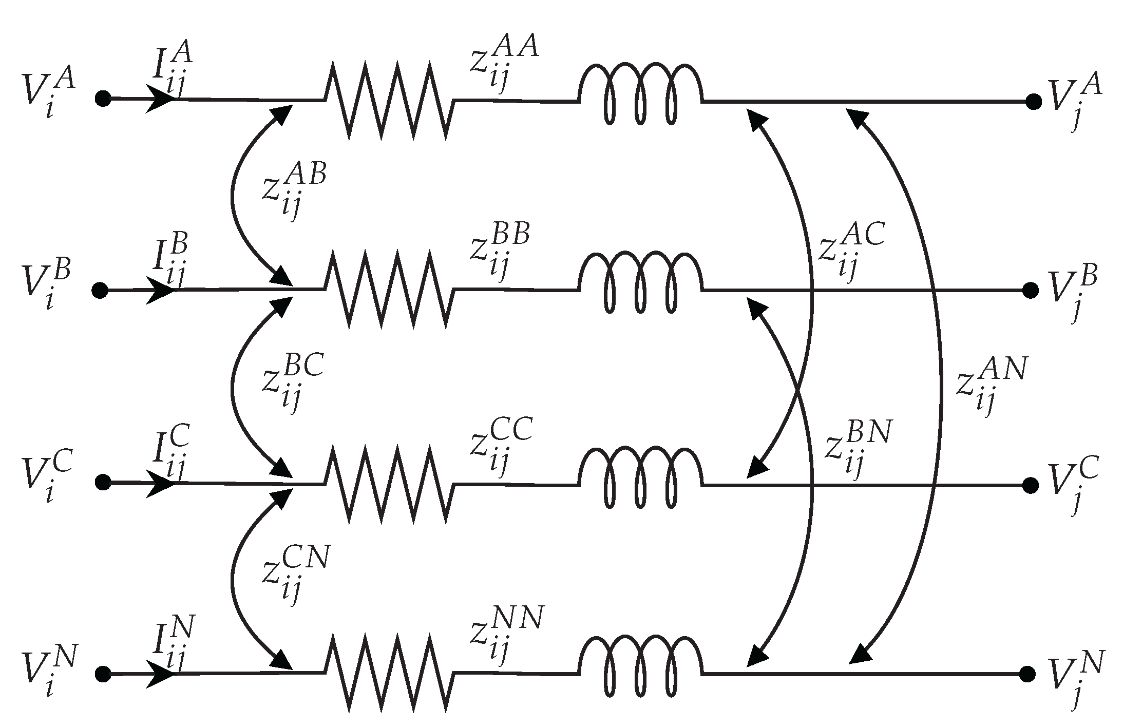
• Model of three-phase distribution lines

Distribution lines in three-phase systems are usually non-transposed and feed unbalanced loads. Therefore, in addition to taking into account the return path of unbalanced currents, the parameters of self- and mutual impedance of the conductors must be considered [66].

Figure 1 shows a three-phase distribution line connecting nodes i and j, as well as the self-impedances (i.e., $Z_{ij}^{ff}$) and mutual impedances (between the conductor in phase f and the conductor in phase g, i.e., $Z_{ij}^{fg}$) of each conductor per phase f. This network segment features three phases and a neutral wire, which means that it is a three-phase four-wire line. When Kirchhoff’s second Law is applied to the circuit depicted in Figure 1, expression (25) is obtained.

$$\left[\begin{array}{c}{V}_i^A\\ V_i^B\\ V_i^C\\ V_i^N\end{array}\right]=\left[\begin{array}{c}{V}_j^A\\ V_j^B\\ V_j^C\\ V_j^N\end{array}\right]+\left[\begin{array}{cccc}{z}_{ij}^{AA}& z_{ij}^{AB}& z_{ij}^{AC}& z_{ij}^{AN}\\ z_{ij}^{BA}& z_{ij}^{BB}& z_{ij}^{BC}& z_{ij}^{BN}\\ z_{ij}^{CA}& z_{ij}^{CB}& z_{ij}^{CC}& z_{ij}^{CN}\\ z_{ij}^{NA}& z_{ij}^{NB}& z_{ij}^{NC}& z_{ij}^{NN}\end{array}\right]\left[\begin{array}{c}{I}_{ij}^A\\ I_{ij}^B\\ I_{ij}^C\\ I_{ij}^N\end{array}\right]$$

(25)

This expression can be represented compactly, that is, by means of vectors and matrices, as shown in the following equation:

$${\mathbf{V}}_i^{ABCN}={\mathbf{V}}_j^{ABCN}+{\mathbf{Z}}_{ij}^{ABCN}{\mathbf{I}}_{ij}^{ABCN},$$

(26)

where ${\mathbf{V}}_i^{ABCN}\in {\mathbb{R}}^{4\times 1}$ and ${\mathbf{V}}_j^{ABCN}\in {\mathbb{R}}^{4\times 1}$ are the vectors containing the voltages of nodes i and j per phase, respectively; ${\mathbf{I}}^{ABCN}\in {\mathbb{R}}^{4\times 1}$ denotes the vector containing the current (per phase) flowing through the distribution line that connects nodes i and j; and ${\mathbf{Z}}_{ij}^{ABCN}\in {\mathbb{R}}^{4\times 4}$ is the three-phase impedance matrix that contains the self- and mutual impedance of each conductor per phase and that of the neutral conductor in the distribution line connecting nodes i and j. The components of this matrix can be determined by applying the modified Carson’s equations, which are shown in Equation (27) [66].

$$\begin{array}{c}{z}_{ij}^{ff}=r_{ij}^f+0.09530+j0.012134\left(\ln \frac{1}{GM{R}_{ij}^f}+7.93402\right)\mathsf{\Omega }/\mathrm{mile}\\ z_{ij}^{fg}=0.09530+j0.012134\left(\ln \frac{1}{D^{fg}}+7.93402\right)\mathsf{\Omega }/\mathrm{mile}\end{array}$$

(27)

where $r_{ij}^f$ is the resistance (in $\mathsf{\Omega }/$mile) of the conductor that connects node i to node j in phase f; $GM{R}_{ij}^f$, the geometrical mean radius (in $ft$) of the conductor that connects node i to node j in phase f; and $D^{fg}$, the spacing (in $ft$) between the conductors in phases f and g.

Applying Equation (27) to a three-phase distribution line with a neutral wire results in a matrix of size 4 × 4, as can be seen in Equation (25). For many applications (such as a three-phase power flow), the three-phase impedance matrix must be reduced to a matrix of size 3 × 3 that is based on the self- and mutual equivalent impedances of the conductors per phase, excluding the neutral conductor [66]. To do this, the impedance matrix of the distribution line should be first separated into conductors per phase and neutral conductor, as shown in the following equation:

$${\mathbf{Z}}_{ij}^{ABCN}=\left[\begin{array}{cc}{\mathbf{Z}}_{ij}^{ff}& {\mathbf{Z}}_{ij}^{fN}\\ {\mathbf{Z}}_{ij}^{Nf}& {\mathbf{Z}}_{ij}^{NN}\end{array}\right],$$

(28)

where ${\mathbf{Z}}_{ij}^{ff}\in {\mathbb{R}}^{3\times 3}$ is the component of the impedance matrix that relates the phases to each other; ${\mathbf{Z}}_{ij}^{fN}\in {\mathbb{R}}^{1\times 3}={\left({\mathbf{Z}}_{ij}^{Nf}\in {\mathbb{R}}^{3\times 1}\right)}^T$, the component of the impedance matrix that relates the phases to the neutral conductor and vice versa; and ${\mathbf{Z}}_{ij}^{NN}\in {\mathbb{R}}^{1\times 1}$, the component of the impedance matrix associated with the neutral conductor.

Once the matrix is divided into conductors per phase and neutral conductor, Kron’s reduction method is applied, as shown in Equation (29) [67].

$${\mathbf{Z}}_{ij}^{ABC}={\mathbf{Z}}_{ij}^{ff}-{\mathbf{Z}}_{ij}^{fN}{\left({\mathbf{Z}}_{ij}^{NN}\right)}^{-1}{\mathbf{Z}}_{ij}^{Nf}$$

(29)

The result is a 3 × 3 matrix, as can be seen in Equation (30). This matrix includes, among its parameters, the effect of the neutral conductor.

$${\mathbf{Z}}_{ij}^{ABC}=\left[\begin{array}{ccc}{z}_{ij}^{AA}& z_{ij}^{AB}& z_{ij}^{AC}\\ z_{ij}^{BA}& z_{ij}^{BB}& z_{ij}^{BC}\\ z_{ij}^{CA}& z_{ij}^{CB}& z_{ij}^{CC}\end{array}\right]\mathsf{\Omega }/\mathrm{mile}$$

(30)

In a non-transposed distribution line, the terms on the diagonal of Equation (30) will not be the same, as occurs with the terms outside the diagonal [66]. The impedance matrix, however, will always be symmetrical.

We will use an example to demonstrate the applicability and usability of the modified Carson’s equations and Kron’s reduction method (given by Equations (27) and (29), respectively) in determining the three-phase impedance matrix of a real distribution line.

Let us consider the overhead distribution line in Figure 2, which is a three-phase four-wire line first reported in [68]. Figure 2 shows the spacing between the phase conductors and the neutral conductor. All the distances are expressed in feet (ft).

Table 2. Parametric information of the IEEE ID-500 overhead distribution line.

Parameter	Value	Unit
Conductor size	1/0 AWG	-
Conductor type	ACSR	-
$r_{ij}^f$	1.12000	$\mathsf{\Omega }$/mile
$GM{R}_{ij}^f$	0.00446	$ft$
$D^{AB}$	2.50000	$ft$
$D^{BC}$	4.50000	$ft$
$D^{CA}$	7.00000	$ft$
$D^{AN}$	5.65685	$ft$
$D^{BN}$	4.27200	$ft$
$D^{CN}$	5.00000	$ft$

details the parametric information of the conductors used for this overhead configuration, which corresponds to Configuration 300 of the IEEE 34-node test system [68].

When the modified Carson’s equations are applied using the parameters given in Table 2, we obtain the three-phase impedance matrix shown in Equation (31).

$${\mathbf{Z}}^{ABCN}=\left[\begin{array}{cccc}1.2153+j1.6195& 0.0953+j0.8515& 0.0953+j0.7266& 0.0953+j0.7524\\ 0.0953+j0.8515& 1.2153+j1.6195& 0.0953+j0.7802& 0.0953+j0.7865\\ 0.0953+j0.7266& 0.0953+j0.7802& 1.2153+j1.6195& 0.0953+j0.7674\\ 0.0953+j0.7524& 0.0953+j0.7865& 0.0953+j0.7674& 1.2153+j1.6195\end{array}\right]\mathsf{\Omega }/\mathrm{mile}$$

(31)

When Kron’s reduction method is applied, we obtain the impedance matrix shown in Equation (32), which corresponds to the impedance matrix of Configuration 300 of the IEEE 34-node test system reported in [69].

$${\mathbf{Z}}^{ABC}=\left[\begin{array}{ccc}1.3238+j1.3569& 0.2101+j0.5779& 0.2066+j0.4591\\ 0.2101+j0.5779& 1.3368+j1.3343& 0.2130+j0.5015\\ 0.2066+j0.4591& 0.2130+j0.5015& 1.3294+j1.3471\end{array}\right]\mathsf{\Omega }/\mathrm{mile}$$

(32)

As demonstrated in the previous example, the modified Carson’s equations and Kron’s reduction method are both reliable tools to model real distribution lines. Therefore, we will use them in this study to determine the impedance matrices of the network segments based on the size of the conductor provided by the master stage.

2.

Model of three-phase loads

The unbalanced loads that can be found in a three-phase distribution system will be modeled based on the analysis of the current they inject into the network, as this current will vary depending on the nature of the load. Therefore, all the loads in a three-phase distribution system are assumed to be connected in a star (Y) or delta ($\Delta$) configuration. Moreover, the loads connected to the demand nodes are assumed to be constant power loads (which is the most critical case in terms of energy losses) [10].

• Solidly-grounded Y-connected loads
  As reported in [70], the three-phase current demanded at node k for a solidly-grounded Y-connected load can be written in a matrix form as shown in the following equation:

  $${\mathbb{I}}_{dk3\phi }=-{\mathbf{diag}}^{-1}\left({\mathbb{V}}_{dk3\phi }^{*}\right){\mathbb{S}}_{dk3\phi }^{*},$$

  (33)

  where ${\mathbb{I}}_{dk3\phi }\in {\mathbb{R}}^{3\times 1}$ is the vector containing the current per phase demanded at node k; $\mathbf{diag}\in {\mathbb{R}}^{3\times 3}$, a positive-definite diagonal matrix; ${\mathbb{V}}_{dk3\phi }\in {\mathbb{R}}^{3\times 1}$, a vector containing the voltage per phase demanded at node k; and ${\mathbb{S}}_{dk3\phi }\in {\mathbb{R}}^{3\times 1}$, the vector containing the complex power per phase demanded at node k.
• $\Delta$-connected loads
  According to [70], the three-phase current demanded at node k for a $\Delta$-connected load can be expressed in a matrix form as shown in the following equation:

  $${\mathbb{I}}_{dk3\phi }=-({\mathbf{diag}}^{-1}\left(\mathbf{M}{\mathbb{V}}_{dk3\phi }^{*}\right)+{\mathbf{diag}}^{-1}\left({\mathbf{M}}^T{\mathbb{V}}_{dk3\phi }^{*}\right)\mathbf{H}){\mathbb{S}}_{dk3\phi }^{*},$$

  (34)

  where matrices $\mathbf{H}$ and $\mathbf{M}$ have the following structure:
  $$\mathbf{H}=\left[\begin{array}{ccc}0& 0& 1\\ 1& 0& 0\\ 0& 1& 0\end{array}\right],\mathbf{M}=\left[\begin{array}{ccc}1& -1& 0\\ 0& 1& -1\\ -1& 0& 1\end{array}\right].$$

  .

Remark 1.

When the modified Carson’s equations are applied to a three-phase three-wire distribution system (i.e., a system with only three phases), an impedance matrix of the form shown in Equation (30) is obtained.

3.3.2. Three-Phase Version of the Backward/Forward Sweep Power Flow Method

After the key elements to solve the power flow problem in three-phase systems (i.e., distribution lines and unbalanced loads) have been modeled, a recursive formulation must be developed to find an exact solution to the power flow problem given by Equation (5) [10]. In this study, the power flow is expanded using the three-phase version of the backward/forward sweep power flow method [10,23], which was selected due to its excellent convergence towards the solution and short processing times. It was also selected because its mathematical formulation considers the currents flowing through the network segments, which is an important constraint when solving the optimal conductor selection problem, as shown in Equation (6). This method is based on Equation (35).

$${\mathbb{V}}_{d3\phi }=-{\mathbf{Z}}_{dd3\phi }\left[\begin{array}{c}{\mathbf{A}}_{d3\phi }{\mathbf{Y}}_{p3\phi }{\mathbf{A}}_{s3\phi }^T{\mathbb{V}}_{s3\phi }-{\mathbb{I}}_{d3\phi }\end{array}\right]$$

(35)

In this equation, ${\mathbb{V}}_{d3\phi }\in {\mathbb{R}}^{3(n-1)\times 1}$ is the vector containing the three-phase voltage at the load nodes, i.e., the variables of interest. ${\mathbf{A}}_{s3\phi }\in {\mathbb{R}}^{3\times 3b}$ denotes the component of the three-phase incidence matrix that relates the generation nodes to each other, while ${\mathbf{A}}_{d3\phi }\in {\mathbb{R}}^{3(n-1)\times 3b}$ is the component of the three-phase incidence matrix that relates the demand nodes to each other. ${\mathbf{Y}}_{p3\phi }\in {\mathbb{R}}^{3b\times 3b}$ is the inverse of the primitive three-phase impedance matrix (${\mathbf{Z}}_{p3\phi }\in {\mathbb{R}}^{3b\times 3b}$), which contains the impedance matrices of all the network segments in the system. Additionally, ${\mathbb{V}}_{s3\phi }\in {\mathbb{R}}^{3\times 1}$ denotes the vector containing the three-phase voltage at the slack node, which is a known parameter to solve the power flow problem. ${\mathbb{I}}_{d3\phi }\in {\mathbb{R}}^{3(n-1)\times 1}$ is the vector containing the net three-phase currents injected into the demand nodes. Finally, ${\mathbf{Z}}_{dd3\phi }={\left[{\mathbf{A}}_{d3\phi }{\mathbf{Y}}_{p3\phi }{\mathbf{A}}_{d3\phi }^T\right]}^{-1}$.

All the demanded three-phase voltages can be calculated using Equation (35). However, to estimate the demanded three-phase current (i.e., ${\mathbb{I}}_{d3\phi }$), the type of load connection (Y or $\Delta$) must be considered in Equation (35), as shown in Equations (33) and (34).

To solve Equation (35), an iterative counter (t) is added to determine the final demanded three-phase voltages based on a starting point, which is usually the voltage at the slack node, i.e., ${\mathbb{V}}_{d3\phi }^0={\mathbf{1}}_{d3\phi }{\mathbb{V}}_{s3\phi }$. Thus, the equation representing the three-phase power flow (35) is solved recursively as defined in Equation (36).

$${\mathbb{V}}_{d3\phi }^{t+1}=-{\mathbf{Z}}_{dd3\phi }\left[\begin{array}{c}{\mathbf{A}}_{d3\phi }{\mathbf{Y}}_{p3\phi }{\mathbf{A}}_{s3\phi }^T{\mathbb{V}}_{s3\phi }-{\mathbb{I}}_{d3\phi }^t\end{array}\right]$$

(36)

The iterative process to solve Equation (36) ends when the convergence criterion shown in Equation (37) is met.

$$\max \left\{\begin{array}{c}\left|\right|{\mathbb{V}}_{d3\phi }^{t+1}|-|{\mathbb{V}}_{d3\phi }^t\left|\right|\end{array}\right\}\le ϵ$$

(37)

where $ϵ$ is the maximum allowable error between two consecutive iterations, which takes a value of $1\times {10}^{-10}$, as recommended in [71].

Remark 2.

The convergence of the backward/forward sweep power flow method can be demonstrated by utilizing the characteristics of the incidence matrix while applying Banach’s fixed-point theorem [72].

Our interest, however, is to solve the complex power balance problem stated in Equation (5), which is time-dependent. Therefore, the iterative equation obtained for the backward/forward sweep power flow method in its three-phase version is expanded by including a time variable (h), which results in the recursive formula shown in Equation (38).

$${\mathbb{V}}_{d3\phi ,h}^{t+1}=-{\mathbf{Z}}_{dd3\phi }\left[\begin{array}{c}{\mathbf{A}}_{d3\phi }{\mathbf{Y}}_{p3\phi }{\mathbf{A}}_{s3\phi }^T{\mathbb{V}}_{s3\phi ,h}-{\mathbb{I}}_{d3\phi ,h}^t\end{array}\right]$$

(38)

Importantly, the values of matrix ${\mathbf{Y}}_{p3\phi }$ are calculated by means of the modified Carson’s equations and Kron’s reduction method—see Equations (27) and (29)—depending on the conductor sizes available for installation and the candidate solutions provided by the master stage. Similarly, ${\mathbb{I}}_{d3\phi ,h}$ is determined based on the three-phase complex power demanded at time period h (i.e., ${\mathbb{S}}_{d3\phi ,h}$)—see Equations (33) and (34)—which will depend on the connections per phase reported by each individual in the master stage. Also, the solution to (38) is obtained when the convergence criterion defined in Equation (37) is met, extending said criterion to the time domain, that is, $max\left\{\begin{array}{c}\left|\right|{\mathbb{V}}_{d3\phi ,h}^{t+1}|-|{\mathbb{V}}_{d3\phi ,h}^t\left|\right|\end{array}\right\}\le ϵ$.

The component of the objective function associated with the costs of energy losses in the system must also be calculated after solving the multi-period three-phase power flow, which is key to solving the problem addressed in this paper. For this purpose, the sum of the powers dissipated by the distribution lines is computed according to the Joule effect, as shown in Equation (39) [23].

$${\mathbb{P}}_{\mathrm{loss},h}=\mathrm{real}\left\{\begin{array}{c}{\mathbb{J}}_{3\phi ,h}^T{\mathbf{Z}}_{p3\phi }{\mathbb{J}}_{3\phi ,h}^{*}\end{array}\right\}$$

(39)

where ${\mathbb{P}}_{\mathrm{loss},h}$ denotes the total active power losses in the system at time period h; and ${\mathbb{J}}_{3\phi ,h}\in {\mathbb{R}}^{3b\times 1}$ represents the three-phase current flowing through the network segments at time period h, which is expressed as shown in Equation (40) by means of Ohm’s law [10].

$${\mathbb{J}}_{3\phi ,h}={\mathbb{Y}}_{p3\phi }{\mathbb{E}}_{3\phi ,h}$$

(40)

where ${\mathbb{E}}_{3\phi ,h}\in {\mathbb{R}}^{3b\times 1}$ denotes the three-phase voltage drop in the distribution lines of the system at time period h, which can be written in terms of power generation and demand using the three-phase incidence matrix, as indicated in Equation (41) [10].

$${\mathbb{E}}_{3\phi ,h}={\mathbf{A}}_{s3\phi }^T{\mathbb{V}}_{s3\phi ,h}+{\mathbf{A}}_{d3\phi }^T{\mathbb{V}}_{d3\phi ,h}$$

(41)

Finally, the energy losses in the system determined by the three-phase version of the backward/forward sweep power flow method are calculated using the following equation:

$${\mathbb{E}}_{loss}=\sum _{h\in \mathcal{H}}{\mathbb{P}}_{\mathrm{loss},h}\Delta h,$$

(42)

where ${\mathbb{E}}_{\mathrm{loss}}$ denotes the energy losses in the system.

Once the power flow problem in the complex domain is solved for each time period h, as shown in Equation (38), and the total energy losses in the system in the time period under analysis are determined, as shown in Equation (42), the fitness function is calculated for each individual provided by the master stage. A fitness function is a modification of the objective function which is frequently employed when metaheuristic techniques are used to restrict the optimization process to only feasible solutions [73,74]. One of the main advantages of using a fitness function instead of the original objective function is that it makes it easier for the metaheuristic optimization algorithm to explore and exploit the solution space effectively, thus increasing the likelihood of finding a global optimal solution that respects the constraints set forth in the mathematical model [75]. The fitness function proposed in this study to solve the optimal conductor selection and phase-balancing problems is given by the following equation:

$$\begin{array}{cc}\hfill F_f=A_{\mathrm{cost}}& -{\alpha }_1\underset{h\in \mathcal{H}}{min}\left\{0,\underset{k\in \mathcal{N}}{min}\left(\right|{\mathbb{V}}_{d3\phi ,h}\left|\right)-V_{min}\right\}\hfill \\ \hfill & +{\alpha }_2\underset{h\in \mathcal{H}}{max}\left\{0,\underset{3\phi \in A,B,C}{max}\left(\right|{\mathbb{J}}_{3\phi ,h}\left|\right)-I_{max}\right\},\hfill \end{array}$$

(43)

where ${\alpha }_1$ is a penalty factor associated with the violation of the lower voltage regulation bound and is assigned a value of $100\times {10}^4$ US$/V, and ${\alpha }_2$ denotes a penalty factor associated with the violation of the thermal limits in all the distribution lines that make up the system and is assigned a value of $100\times {10}^4$ US$/A. Importantly, when the solution obtained by an individual is feasible and within the solution space, both the original objective function and the fitness function yield the same value.

Algorithm 2 presents the process followed by the three-phase version of the backward/forward sweep power flow method to solve the power flow problem and assess the value of the fitness function.

Algorithm 2 Solution to the multi-period three-phase power flow problem using the backward/forward sweep power flow method in order to calculate the fitness function of the optimization problem under study.

4. Three-Phase Test Systems and Additional Considerations

This section presents the main characteristics of the two three-phase test systems (i.e., the 8- and 25-node test systems) that were used to validate the master–slave methodology proposed in this study to solve the optimal conductor selection and phase-balancing problems in unbalanced distribution networks. Both test systems have a radial topology and were initially reported in [10].

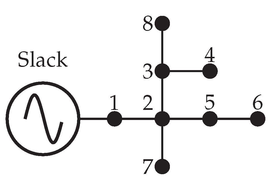
4.1. 8-Node Test System

This unbalanced three-phase test system consists of 7 distribution lines and 8 nodes, and it has a radial topology that operates at a nominal line-to-line voltage of 11 kV at the substation node. Its electrical configuration is illustrated in Figure 3. In the peak load scenario, the power consumption of this system is $\left(1005+j485\right)$kVA for phase A, $\left(785+j381\right)$kVA for phase B, and $\left(1696+j821\right)$kVA for phase C.

Table 3. Parametric information about the 8-node test system (all powers in kW and kvar).

Branch	Node i	Node j	$L_{\mathit{ij}}$ (km)	$P_{\mathrm{jA}}$	$Q_{\mathrm{jA}}$	$P_{\mathrm{jB}}$	$Q_{\mathrm{jB}}$	$P_{\mathrm{jC}}$	$Q_{\mathrm{jC}}$
1	1	2	1	519	250	259	126	515	250
2	2	3	1	0	0	259	126	486	235
3	2	5	1	0	0	0	0	226	109
4	2	7	1	486	235	0	0	0	0
5	3	4	1	0	0	0	0	324	157
6	3	8	1	0	0	267	129	0	0
7	5	6	1	0	0	0	0	145	70

details the parametric information about its distribution lines (i.e., number of lines and length) and the complex power consumption per phase. This information was taken from [10].

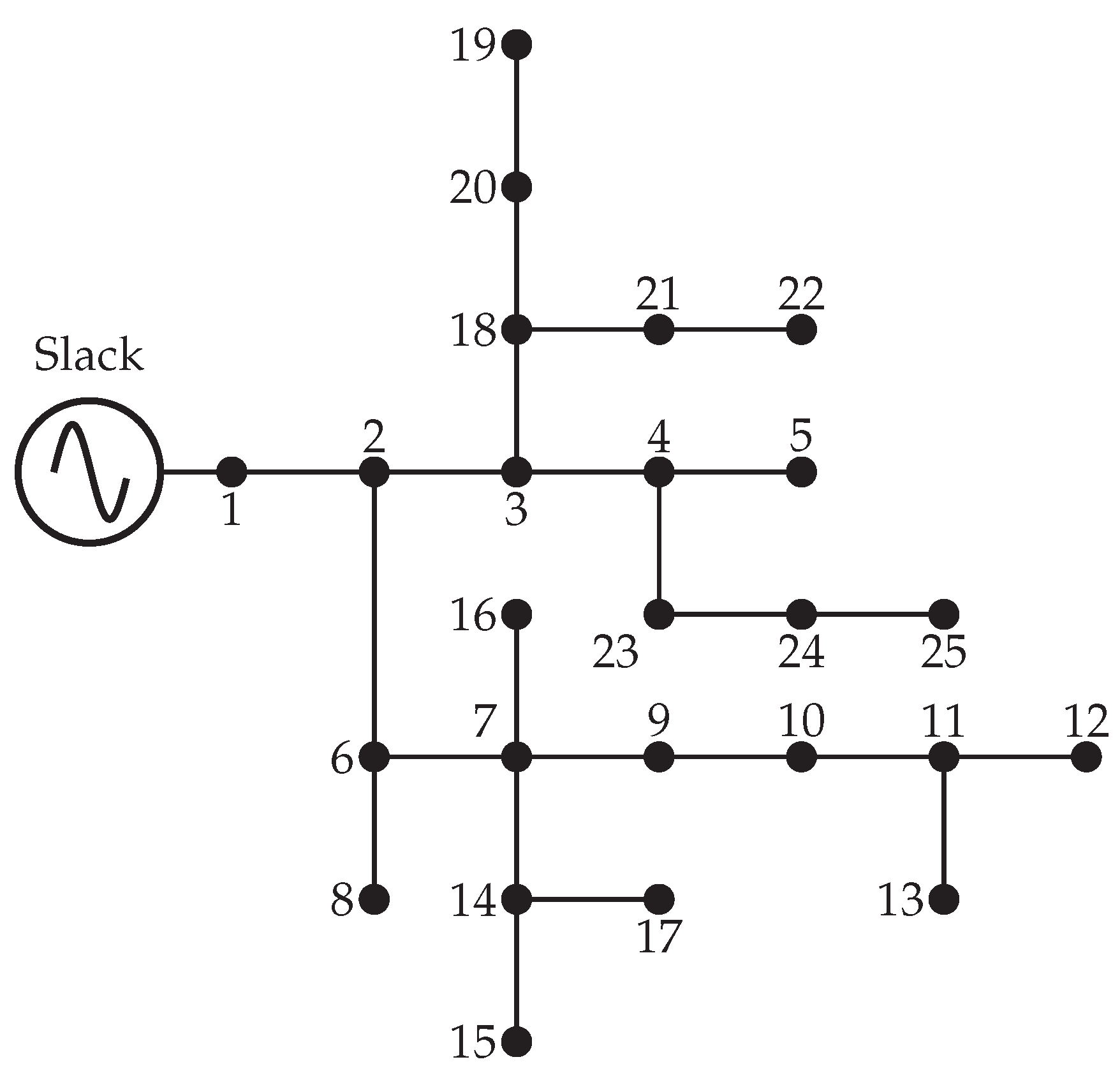
4.2. 25-Node Test System

This unbalanced three-phase test system consists of 24 distribution lines and 25 nodes, and it has a radial topology that operates at a nominal line-to-line voltage of 4.16 kV at the substation node. Its electrical configuration is shown in Figure 4. In the peak load scenario, the power consumption of this system is $\left(946+j648\right)$kVA for phase A, $\left(573.6+j430.6\right)$kVA for phase B, and $\left(771.8+j554\right)$kVA for phase C.

Table 4. Parametric information about the 25-node test system (all powers in kW and kvar).

Branch	Node i	Node j	$L_{\mathit{ij}}$ (km)	$P_{\mathrm{jA}}$	$Q_{\mathrm{jA}}$	$P_{\mathrm{jB}}$	$Q_{\mathrm{jB}}$	$P_{\mathrm{jC}}$	$Q_{\mathrm{jC}}$
1	1	2	0.3048	0	0	0	0	0	0
2	2	3	0.1524	36	21.6	28.8	19.2	42	26.4
3	2	6	0.1524	43.2	28.8	33.6	24	30	30
4	3	4	0.1524	57.6	43.2	4.8	3.4	48	30
5	3	18	0.1524	57.6	43.2	38.4	28.8	48	36
6	4	5	0.1524	43.2	28.8	28.8	19.2	36	24
7	4	23	0.1219	8.6	64.8	4.8	3.8	60	42
8	6	7	0.1524	0	0	0	0	0	0
9	6	8	0.3048	43.2	28.8	28.8	19.2	3.6	2.4
10	7	9	0.1524	72	50.4	38.4	28.8	48	30
11	7	14	0.1524	57.6	36	38.4	28.8	60	42
12	7	16	0.1524	57.6	4.3	3.8	28.8	48	36
13	9	10	0.1524	36	21.6	28.8	19.2	32	26.4
14	10	11	0.0914	50.4	31.7	24	14.4	36	24
15	11	12	0.0610	57.6	36	48	33.6	48	36
16	11	13	0.0610	64.8	21.6	33.6	21.1	36	24
17	14	15	0.0914	7.2	4.3	4.8	2.9	6	3.6
18	14	17	0.0914	57.6	43.2	33.6	24	54	38.4
19	18	20	0.1524	50.4	36	38.4	28.8	54	38.4
20	18	21	0.1219	5.8	4.3	3.4	2.4	5.4	3.8
21	20	19	0.1219	8.6	6.5	4.8	3.4	6	4.8
22	21	22	0.1219	72	50.4	57.6	43.2	60	48
23	23	24	0.1219	50.4	36	43.2	30.7	4.8	3.6
24	24	25	0.1219	8.6	6.5	4.8	2.9	6	4.2

presents the parametric information about its distribution lines (i.e., number of lines and length) and the complex power consumption per phase. This parametric information was taken from [10].

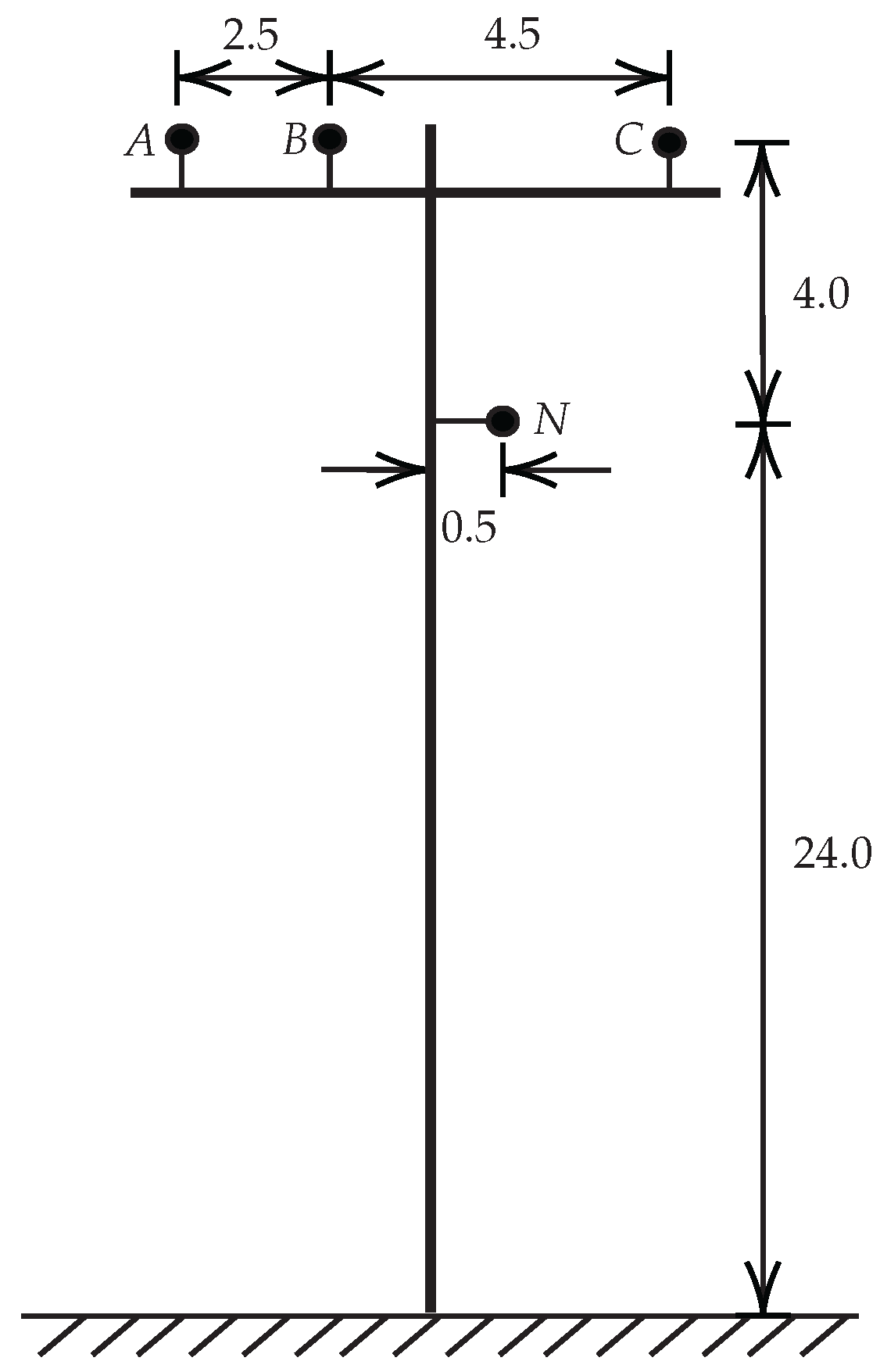
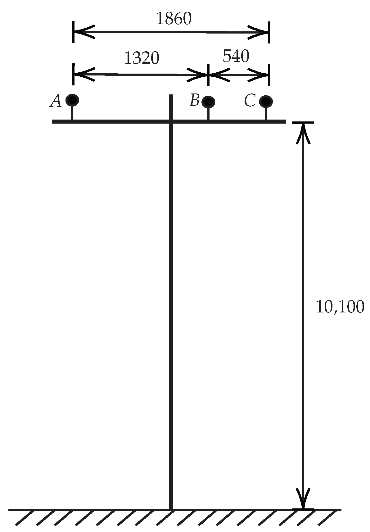
4.3. Overhead Line Configuration and Set of Available Conductors

To solve the problem addressed in this paper, all the distribution lines in the test systems described above are assumed to be three-phase, three-wire lines. Their geometrical configuration is illustrated in Figure 5. This type of overhead line configuration is known as LA202, and it is commonly used by Enel Codensa, an electricity distribution company located in Bogotá (Colombia) [76]. All the distances in Figure 5 are expressed in millimeters (mm) and were taken from [77].

To determine the optimal conductor size that the master stage should assign to each distribution line in each test system under analysis, we considered eight different types of conductors (i.e., $N_c^{ava}$), which are presented in

Table 5. Parametric information about the conductors considered for the two test systems.

Conductor Size	r ($\mathsf{\Omega }$/km)	$\mathit{GMR}$ (mm)	I${}_{max}$ (A)	$\mathit{Cost}$ (USD/km)
1	1.0501	1.2741	180	1986
2	0.8575	1.2741	200	2790
3	0.6959	1.3594	230	3815
4	0.5561	1.5545	270	5090
5	0.4493	1.8288	300	8067
6	0.3679	2.4811	340	12,673
7	0.1609	8.4734	600	23,419
8	0.1155	9.5402	720	30,070

.

Table 5 details several aspects of the eight available conductor sizes (from left to right): size number, resistance (r), geometrical mean radius ($GMR$), thermal current limit ($I_{max}$), and cost per kilometer ($Cost$). The information on the resistance, GMR, and thermal current limit of each conductor corresponds to that of real conductors and can be found in [66]. Likewise, the cost of each conductor was taken from [13].

Based on the information in Figure 5 and Table 5, we calculated the impedance matrix of each of the eight conductor sizes considered in this study. Equations (27) and (29) were used for such purpose. The resulting impedance matrices are shown in

Table 6. Impedance matrix of the conductors considered for the two test systems.

Conductor Size ($\mathsf{\Omega }/$km)
	$1.1093+j1.0112$	$0.0592+j0.4877$	$0.0592+j0.4618$
1	$0.0592+j0.4877$	$1.1093+j1.0112$	$0.0592+j0.5551$
	$0.0592+j0.4618$	$0.0592+j0.5551$	$1.1093+j1.0112$
	$0.9167+j1.0112$	$0.0592+j0.4877$	$0.0592+j0.4618$
2	$0.0592+j0.4877$	$0.9167+j1.0112$	$0.0592+j0.5551$
	$0.0592+j0.4618$	$0.0592+j0.5551$	$0.9167+j1.0112$
	$0.7552+j1.0063$	$0.0592+j0.4877$	$0.0592+j0.4618$
3	$0.0592+j0.4877$	$0.7552+j1.0063$	$0.0592+j0.5551$
	$0.0592+j0.4618$	$0.0592+j0.5551$	$0.7552+j1.0063$
	$0.6153+j0.9962$	$0.0592+j0.4877$	$0.0592+j0.4618$
4	$0.0592+j0.4877$	$0.6153+j0.9962$	$0.0592+j0.5551$
	$0.0592+j0.4618$	$0.0592+j0.5551$	$0.6153+j0.9962$
	$0.5085+j0.9839$	$0.0592+j0.4877$	$0.0592+j0.4618$
5	$0.0592+j0.4877$	$0.5085+j0.9839$	$0.0592+j0.5551$
	$0.0592+j0.4618$	$0.0592+j0.5551$	$0.5085+j0.9839$
	$0.4271+j0.9609$	$0.0592+j0.4877$	$0.0592+j0.4618$
6	$0.0592+j0.4877$	$0.4271+j0.9609$	$0.0592+j0.5551$
	$0.0592+j0.4618$	$0.0592+j0.5551$	$0.4271+j0.9609$
	$0.2202+j0.8683$	$0.0592+j0.4877$	$0.0592+j0.4618$
7	$0.0592+j0.4877$	$0.2202+j0.8683$	$0.0592+j0.5551$
	$0.0592+j0.4618$	$0.0592+j0.5551$	$0.2202+j0.8683$
	$0.1747+j0.8594$	$0.0592+j0.4877$	$0.0592+j0.4618$
8	$0.0592+j0.4877$	$0.1747+j0.8594$	$0.0592+j0.5551$
	$0.0592+j0.4618$	$0.0592+j0.5551$	$0.1747+j0.8594$

.

The primitive impedance matrix (${\mathbf{Y}}_{p3\phi }$) of each test system can be determined based on the set of conductor sizes provided by the master stage. Then, the three-phase power flow can be evaluated in order to find the value of the fitness function.

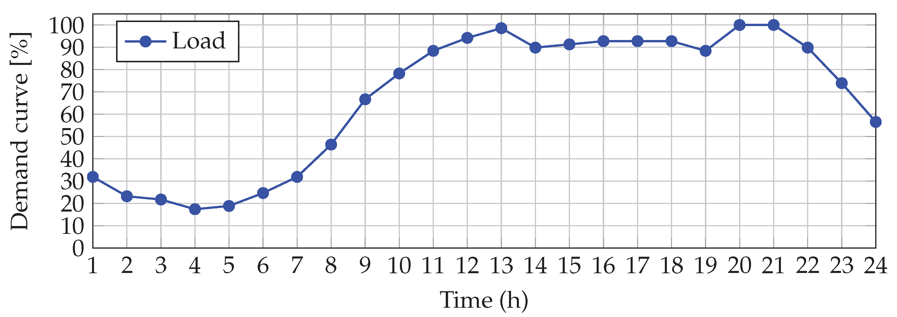
4.4. Load Profile Curve

To assess the impact of the conductor selection and phase-balancing on the test systems describe above, we employed a typical demand curve in Colombia, which is illustrated in Figure 6. Data on variations in consumption can be found in [78]. As observed in Figure 6, the peak demand occurs at 20 and 21 h.

In addition, to assess the value of the objective function defined in Equation (1), the energy cost is assumed to be 0.1390 USD/kWh, which corresponds to the average energy cost in Bogotá (Colombia) in May 2019 [79]. The number of days considered here is 365 (a calendar year), and the time period during which power consumption remains constant for the three-phase power flow ($\Delta h$) is one hour. The voltage regulation limits are set at $\pm 10\%$, as established by the CREG in Resolution 025 of 1995 [80]. Additionally, the cost of reconfiguring the phases of the system by a work crew is set at 100 USD for each node requiring intervention, as recommended by the authors of [26].

5. Numerical Results and Discussion

This section presents the numerical validation of the master–slave methodology (proposed here to solve the optimal conductor selection and phase-balancing problems in the 8-node and 25-node test systems) considering a one-year operation scenario. To demonstrate the efficiency of the proposed solution methodology, we compared it with two other metaheuristic optimization techniques that have been employed to solve the phase-balancing problem in distribution systems: the Hurricane-based Optimization Algorithm (HOA) [24] and the Sine Cosine Algorithm (SCA) [26].

Additionally, to define a baseline for comparison, we used 10 individuals and 1000 iterations in all the computational simulations of the three optimization algorithms. Moreover, we considered 100 consecutive evaluations in order to find the best, average, and worst values of the objective function. Likewise, we calculated the standard deviation of the 100 solutions, as well as the average time required by each algorithm to find both the set of conductors for the distribution lines and the set of connections at the demand nodes for the two test systems under analysis.

The optimization model defined in Equations (1)–(14) was implemented and solved in MATLAB (version 2022a) using native scripts on a desktop computer with an Intel(R) Core(TM) i9-11900 CPU@2.50 GHz processor, 64.0 GB of RAM, and 64-bit Windows 10 Pro.

5.1. Results in the 8-Node Test System

5.1.1. Numerical Results

Table 7. Numerical results in the 8-node test system (all units in USD/year).

Method	Caliber	${\mathit{A}}_{\mathit{cost}}$	${\mathit{f}}_1$	${\mathit{f}}_2$	${\mathit{f}}_3$
	Connection
SCA	$\left\{5,2,1,1,1,1,1\right\}$	125,351.07	62,690.07	62,361.00	300.00
	$\left\{2,1,3,1,4,1,1\right\}$
HOA	$\left\{5,2,1,1,1,1,1\right\}$	125,348.49	62,687.49	62,361.00	300.00
	$\left\{6,1,5,1,4,1,1\right\}$
SSA	$\left\{5,2,1,1,1,1,1\right\}$	125,348.49	62,687.49	62,361.00	300.00
	$\left\{6,1,5,1,2,1,1\right\}$

presents the numerical results obtained by the discrete version of the SSA and the two other metaheuristic techniques (used for comparison) when they solved the optimal conductor selection and phase-balancing problems in the 8-node test system.

In said table, the proposed SSA and the HOA both yielded the (same) best operating cost, i.e., 125,348.49 USD/year. Meanwhile, the SCA produced the worst value in this regard (i.e., 125,351.07 USD/year), which represents a difference of 2.58 USD/year compared to the solution obtained by the discrete version of the SSA. The three methods compared here provided the same set of conductor sizes, with an investment cost of 62,361.00 USD/year. Finally, all the optimization methodologies made only three changes to balance the system. Nevertheless, the set of connections determined by the HOA and the SSA were found to better distribute the load within the phases of the system, which is reflected in the lower cost associated with energy losses (62,687.49 USD/year) and confirms the difference of 2.58 USD/year mentioned above.

Figure 7 compares the initial and final unbalance percentages (total and per phase) over a one-day operation in the 8-node test system considering the set of connections provided by the proposed SSA. As observed, there was a 25.3% reduction in the system’s average unbalance and 5.51%, 30.03%, and 40.37% reductions in the unbalance in phases A, B, and C, respectively. According to the phase-balancing results, the system’s average and per-phase unbalance decreased significantly, which allows the system to reach an optimal operating point.

5.1.2. Statistical Analysis

To validate the effectiveness and robustness of the SSA (in its discrete version) to solve the problem addressed in this paper, 100 consecutive executions of the master–slave methodology were carried out in the 8-node test system. According to the results, which are reported in

Table 8. Statistical data on the performance of the three methodologies in the 8-node test system (all units in USD/year).

Method	Best	Mean	Worst	SD	Avg. Time (s)
SCA	125,351.07	131,673.85	146,483.13	3602.51	57.57
HOA	125,348.49	130,929.42	140,533.94	2911.76	60.25
SSA	125,348.49	128,498.41	130,443.99	1506.07	57.47

, the SSA performed better than the HOA and the SCA when they solved the optimal conductor selection and phase-balancing problems in the 8-node test system. Regarding the best response, the SSA and the HOA showed an improvement of 0.0021%, i.e., 2.5 USD/year, compared to the SCA. Likewise, in terms of the average and worst responses, the SSA presented an improvement of approximately 2431 USD/year and 10,089.95 USD/year, respectively, compared to the HOA and of approximately 3175.44 USD/year and 16,039.14 USD/year, respectively, compared to the SCA. This demonstrates that, compared to alternative solution approaches like the HOA and the SCA, the proposed methodology is superior in finding a solution to the problem under analysis in terms of the best, average, and worst values of the objective function.

As reported in Table 8, the SSA presented a standard deviation of 1506.07 USD/year, which is a difference of 1.17% compared to the average value. It also represents an improvement of approximately 1405.69 USD/year over the standard deviation of the HOA and of 2096.44 USD/year over that of the SCA. This demonstrates the repeatability of the SSA in solving the optimal conductor selection and phase-balancing problems because, when it is executed multiple times in the 8-node test system, it is likely to produce the average value or one very close to it within a range of less than 1507 USD/year.

Additionally, the processing time required by each one of the three methodologies to solve the problem under study in the 8-node test system was approximately 60 s. We consider this a really fast processing time, given that 24 three-phase power flows were evaluated for each combination of sizes per conductor and phase connections per node provided by each algorithm. This means that approximately 240,000 three-phase power flows were evaluated for a population of 10 individuals and 1000 iterations. Furthermore, the algorithms had to explore and exploit a solution space with a size of ${\left(N_c^{ava}\right)}^b·6^{(n-1)}$, i.e., $8^7·6^7=5.8707\times {10}^{11}$ possible solutions. According to the results, the SSA required the shortest average processing time to find a solution (i.e., 57.47 s), followed by the SCA (57.57 s), and the HOA (60.25 s).

These results demonstrate the efficiency and robustness of the SSA (in its discrete version) to solve the optimal conductor selection and phase-balancing problems because, compared to other solution methodologies, it presented a high repeatability and required a short processing time.

5.1.3. Feasibility Check

The optimal solution provided by the SSA is feasible if it respects the electrical constraints established in the mathematical model defined in Equations (5)–(14), which were considered in the formulation of the fitness function (see Equation (43)). To verify such feasibility, we analyzed the behavior of the maximum three-phase current in the 8-node test system after installing the conductors per phase in each distribution line and establishing the phase connections for each demand node (see Figure 8).

In this test system, the maximum three-phase current was always found in the main feeder, that is, in the distribution line connecting nodes 1 and 2, i.e., distribution line 1. As expected, the three-phase current followed the power demand curve and reached its highest value at 20 and 21 h (peak demand scenario), with a value of 193.75 A for phase A, 216.01 A for phase B, and 219.90 A for phase C.

As observed in Figure 8, the current per phase in all the time periods respected the maximum current constraint because, based on the information provided in Table 7, a conductor of size 5 with a maximum current rating of 300 A was installed in this distribution line. In addition, during the period of peak demand (from 20 to 21 h), the loadability of the conductor in phase A was 64.58%; in phase B, 72%; and, in phase C, 73.3%.

Finally, Figure 9 illustrates the behavior of the minimum voltage per phase in the 8-node test system after the solution provided by the SSA was implemented.

From Figure 9, we may conclude that the minimum voltage per phase respected the voltage regulation constraint in all the time periods because it was always within the $\pm 10\%$ range. Furthermore, from 20 to 21 h (when the system loads demanded the maximum possible power), the minimum voltage in phase A was 0.9591 pu at node 4; in phase B, 0.9463 pu at node 8; and, in phase C, 0.9689 pu at node 4.

5.2. Results in the 25-Node Test System

5.2.1. Numerical Results

Table 9. Numerical results in the 25-node test system (all units in USD/year).

Method	Conductor Size	${\mathit{A}}_{\mathit{cost}}$	${\mathit{f}}_1$	${\mathit{f}}_2$	${\mathit{f}}_3$
	Connection
HOA	$\left\{7,4,5,4,3,1,4,4,1,1,2,1,3,1,2,1\right\}$	98,068.39	45,968.05	51,400.34	700.00
	$\left\{1,2,1,1,1,2,2,2,1,1,6,1,6,1,1,6\right\}$
	$\left\{1,6,1,1,6,1,1,1,6,1,1,1,6,1,1,1\right\}$
SCA	$\left\{7,4,4,1,1,1,1,4,1,4,1,1,1,1,4,1\right\}$	96,404.47	48,661.03	46,843.43	900.00
	$\left\{1,2,1,2,1,1,1,1,1,1,2,1,1,1,2,1\right\}$
	$\left\{1,1,2,3,2,1,2,1,1,1,2,1,2,2,1,1\right\}$
SSA	$\left\{7,4,5,1,2,1,1,4,1,4,1,1,2,1,1,1\right\}$	94,505.81	46,195.44	47,710.37	600.00
	$\left\{1,1,1,1,1,1,1,1,1,1,6,6,1,1,1,6\right\}$
	$\left\{1,1,1,6,1,1,1,6,6,1,1,1,1,1,1,1\right\}$

presents the numerical results obtained by the proposed solution methodology and the two metaheuristic techniques used here for comparison in the 25-node test system.

According to the results presented in said table, the SSA produced the best operating costs, i.e., 94,505.81 USD/year. Meanwhile, the operating costs yielded by the SCA and the HOA were 96,404.47 USD/year and 98,068.39 USD/year, respectively, which represent differences of 1898.66 USD/year and 3562.58 USD/year, respectively, compared to the solution obtained by the SSA in its discrete version. Additionally, even though all the methodologies provided different sets of conductor sizes, lines 1 and 2 presented the same conductor sizes (i.e., 7 and 4) in all the solutions. This is explained by the fact that the largest amount of three-phase current flows through these two lines, as they are the network segments in charge of interconnecting the substation node and the system loads. The SCA provided the lowest investment costs (46,843.43 USD/year). However, although the SSA requires a larger investment (approximately 886.94 USD/year more than the SCA), the latter helps to reduce energy losses over a year of operation, producing savings of roughly 2465.60 USD/year compared to the SCA, which clearly justifies the additional investment in conductors. Finally, the SSA reported the least number of changes to balance the system (only 6), which results in savings of 300 USD/year compared to the SCA and of 100 USD/year compared to the HOA.

As with the previous test system, Figure 10 compares the initial and final unbalance percentages (total and per phase) over a one-day operation in the 25-node test system considering the set of connections provided by the SSA. As observed, there was a 15.29% reduction in the system’s average unbalance and 22.93%, 22.94%, and 0% reductions in the unbalance in phases A, B, and C, respectively. According to the phase-balancing results, the system’s average and per-phase unbalance decreased significantly, which allows the system to reduce its energy losses in one year of operation and, thus, the associated costs.

5.2.2. Statistical Analysis

To validate the effectiveness and robustness of the SSA (in its discrete version), 100 consecutive executions of the proposed methodology were performed in the 25-node test system. According to the results, which are reported in

Table 10. Statistical data on the performance of the three methodologies in the 25-node test system (all units in USD/year).

Method	Best	Mean	Worst	SD	Avg. Time (s)
HOA	98,068.39	106,388.04	117,337.29	4191.39	451.00
SCA	96,404.47	109,539.42	135,192.31	8896.28	446.20
SSA	94,505.81	96,461.04	98,631.18	717.61	526.19

, the SSA performed better than the SCA and the HOA when they solved the optimal conductor selection and phase-balancing problems in the 25-node test system. Regarding the best response, the SSA showed an improvement of 1.97%, i.e., 1898.66 USD/year, over the SCA and an improvement of 3.63%, i.e., 3562.58 USD/year, over the HOA. Also, in terms of the average and worst responses, the SSA showed improvements of approximately 13,078.38 USD/year and 36,561.13 US$/year, respectively, compared to the SCA and of approximately 9927 USD/year and 18,706.11 USD/year, respectively, compared to the HOA. This demonstrates that, compared to other solution approaches like the SCA and the HOA, the proposed methodology is superior in finding a solution to the problem under study in terms of the best, average, and worst values of the objective function.

As reported in Table 10, the SSA obtained a standard deviation of 717.61 USD/year, which represents a difference of 0.74% compared to the average value. It also represents an improvement of approximately 8178.67 USD/year compared to the standard deviation of the SCA and of 3473.78 USD/year compared to the standard deviation of the HOA. This demonstrates the repeatability of the SSA when it solves the optimal conductor selection and phase-balancing problems because, if it is executed multiple times in the 25-node test system, it is likely to produce the average value or one very close to it within a range of less than 718 USD/year.

Regarding processing times, all three methodologies required more than 400 s to solve the problem under analysis in the 25-node test system. We consider this an acceptable processing time given that each algorithm evaluated around 240,000 three-phase power flows. Furthermore, the algorithms had to explore and exploit a solution space with a size of $8^{24}·6^{24}=2.2376\times {10}^{40}$ possible solutions. According to the results, the SSA took the longest average processing time to find a solution (526.19 s), whereas the SCA and the HOA required processing times of 446.20 s and 451 s, respectively. These processing times can be considered negligible with regard to the planning horizon used in this study case (one year of operation), i.e., 31,536,000 s.

These results demonstrate the efficiency and robustness of the SSA (in its discrete version) to solve the optimal conductor selection and phase-balancing problems because it showed a high repeatability compared to the two other solution methodologies.

5.2.3. Feasibility Check

To verify that the optimal solution provided by the SSA is feasible, we analyzed the behavior of the maximum three-phase current in the 25-node test system after installing the conductors per phase in each distribution line and establishing the phase connections for each demand node (see Figure 11).

In this test system, the maximum three-phase current was always found in the main feeder. As in the previous test system, the three-phase current followed the power demand curve and reached its highest value at 20 and 21 h, with a value of 409.44 A for phase A, 398.90 A for phase B, and 409.71 A for phase C.

As observed in Figure 11, the current per phase respected the maximum current constraint in all the time periods because, based on the information provided in Table 9, a conductor of size 7 with a maximum current rating of 600 A was installed in this distribution line. In addition, during the period of peak demand (from 20 to 21 h), the loadability of the conductor in phase A was 68.24%; in phase B, 66.48%; and, in phase C, 68.29%.

Finally, Figure 12 illustrates the behavior of the minimum voltage per phase in the 25-node test system after the solution provided by the SSA was implemented.

Based on Figure 12, we may conclude that the minimum voltage per phase respected the voltage regulation constraint in all the time periods because it was always within the $\pm 10\%$ range. Additionally, from 20 to 21 h, the minimum voltage in phase A was 0.9457 pu at node 12; in phase B, 0.9498 pu at node 13; and, in phase C, 0.9543 pu at node 12.

6. Conclusions and Future Work

In this paper, we presented a master–slave methodology that uses a discrete version of the SSA to solve the optimal conductor selection and phase-balancing problems in three-phase unbalanced electrical distribution systems. In the master stage, the SSA is in charge of defining the set of sizes to be used per conductor in each network segment, as well as the set of connections per phase at the system’s demand nodes. In the slave stage, the three-phase version of the backward/forward sweep power flow method is responsible for calculating the value of the fitness function. The objective function we considered here was the minimization of the total annual operating costs, which include the costs associated with (i) energy losses over one year of operation, (ii) investment in conductors, and (iii) phase-balancing by a work crew.

The numerical results obtained by the proposed solution methodology in the 8- and 25-node test systems demonstrated its applicability and efficiency compared to other methods reported in the specialized literature, such as the HOA and the SCA. The following are the main conclusions in this study:

🗸

In the 8-node test system, the SSA achieved a reduction in total annual operating costs of 0.0021% compared to the SCA. In the 25-node test system, it achieved a reduction of 1.97% compared to the SCA and of 3.63% compared to the HOA.

🗸

The proposed solution methodology presented a low standard deviation when it solved the optimal conductor selection and phase-balancing problems in the 8- and 25-node test systems (1506.07 USD/year and 717.61 USD/year, respectively). These values were lower than those of the two methods used here for comparison (i.e., the SCA and the HOA), which confirms the repeatability and robustness of the proposed SSA when it solves the problem under study. Also, this ensures that, in each evaluation, its solution falls within a range of 1507 USD/year in the 8-node system and of 718 USD/year in the 25-node system with respect to the average value obtained for each system.

🗸

The processing time required by the proposed methodology to find an optimal and feasible solution to the problem under study was 57.47 s in the 8-node test system and 526.19 s in its 25-node counterpart. These processing times are acceptable, considering that the SSA evaluated approximately 240,000 three-phase power flows and explored and exploited a solution space with a size of $5.8707\times {10}^{11}$ in the 8-node test system and of $2.2376\times {10}^{40}$ in the 25-node test system. Therefore, we may conclude that the proposed solution methodology is independent of the number of nodes, as long as the system under study has a radial topology. Nevertheless, if the number of nodes in the system increases, the solution space expands, lengthening the processing time needed to find a solution to the problem. This increase in time, however, is not critical in the planning of three-phase distribution systems because its most important concern is the quality of the solution.

🗸

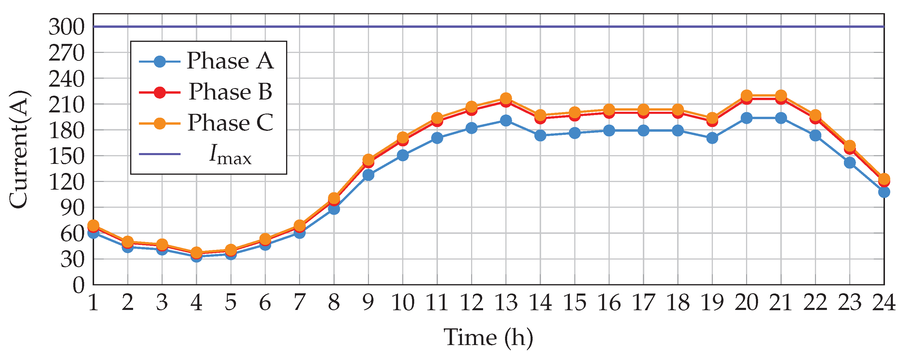
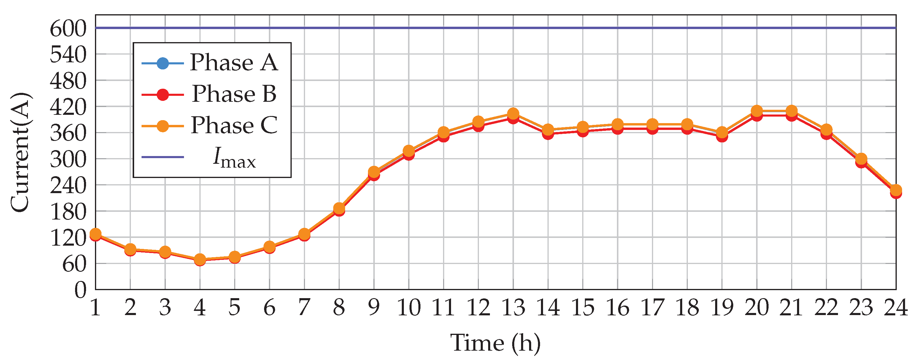
In both test systems, the three-phase current reached its highest value in all the conductors in the system during the period of peak demand (from 20 to 21 h). Particularly, the most critical case was that of distribution line 1, with values of 193.75 A in phase A, 216.01 A in phase B, and 219.90 A in phase C in the 8-node test system and of 409.44 A in phase A, 398.90 A in phase B, and 409.71 A in phase C in the 25-node test system. These results confirm that, in both test systems, the thermal current limit constraint set for the installed conductors was respected because, in the most critical case, the loadability of line 1 in the 8-node test system was 64.58% in phase A, 72% in phase B, and 73.3% in phase C, while that in the 25-node test system was 68.24% in phase A, 66.48% in phase B, and 68.29% in phase C.

🗸

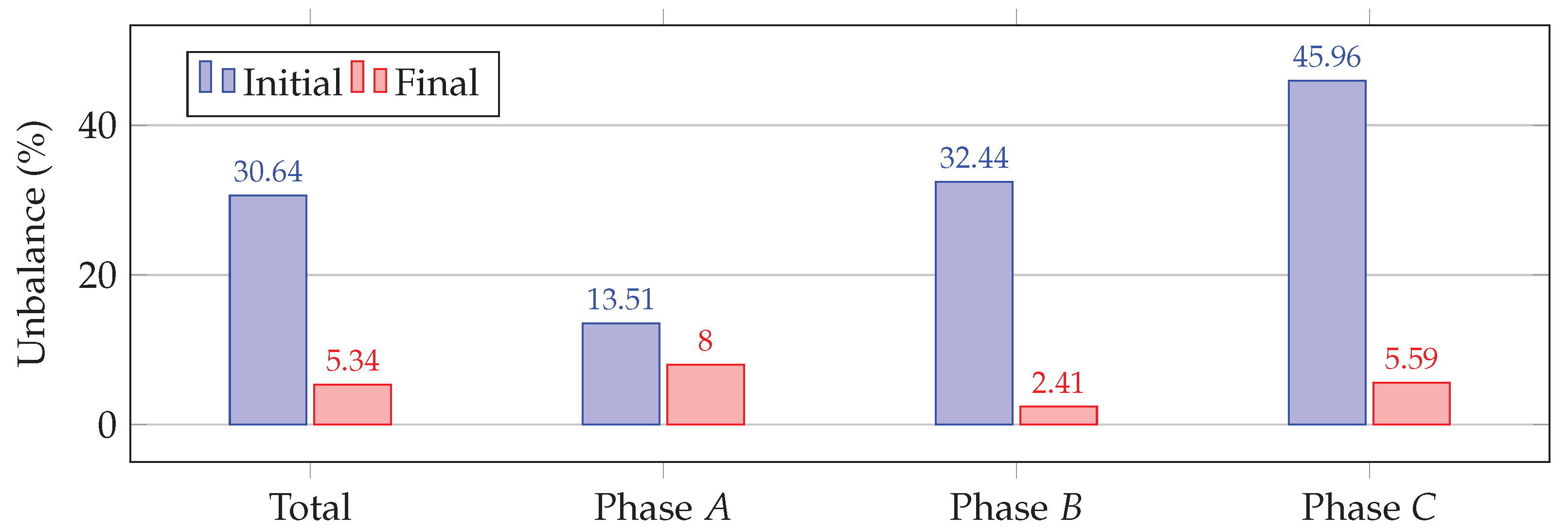
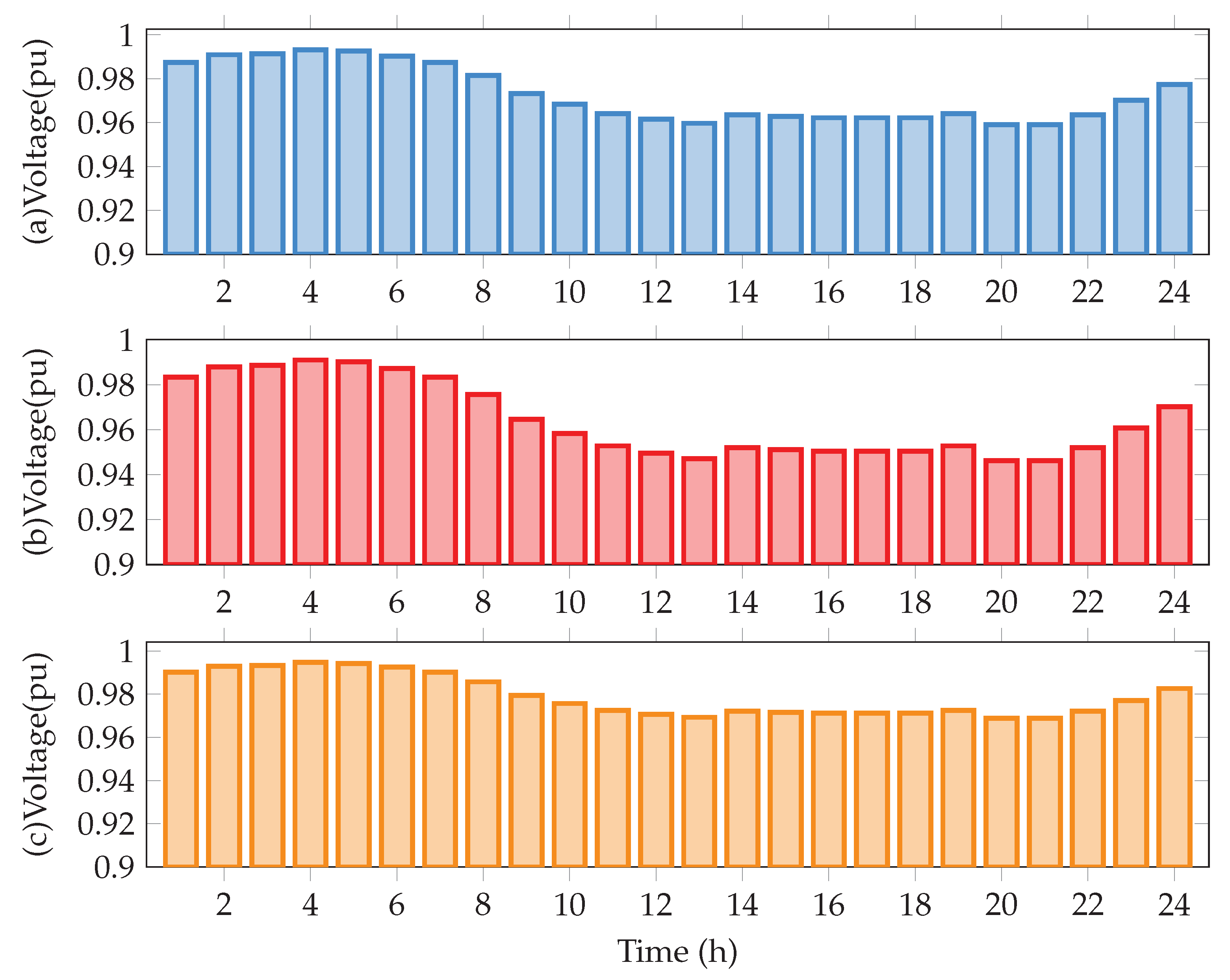
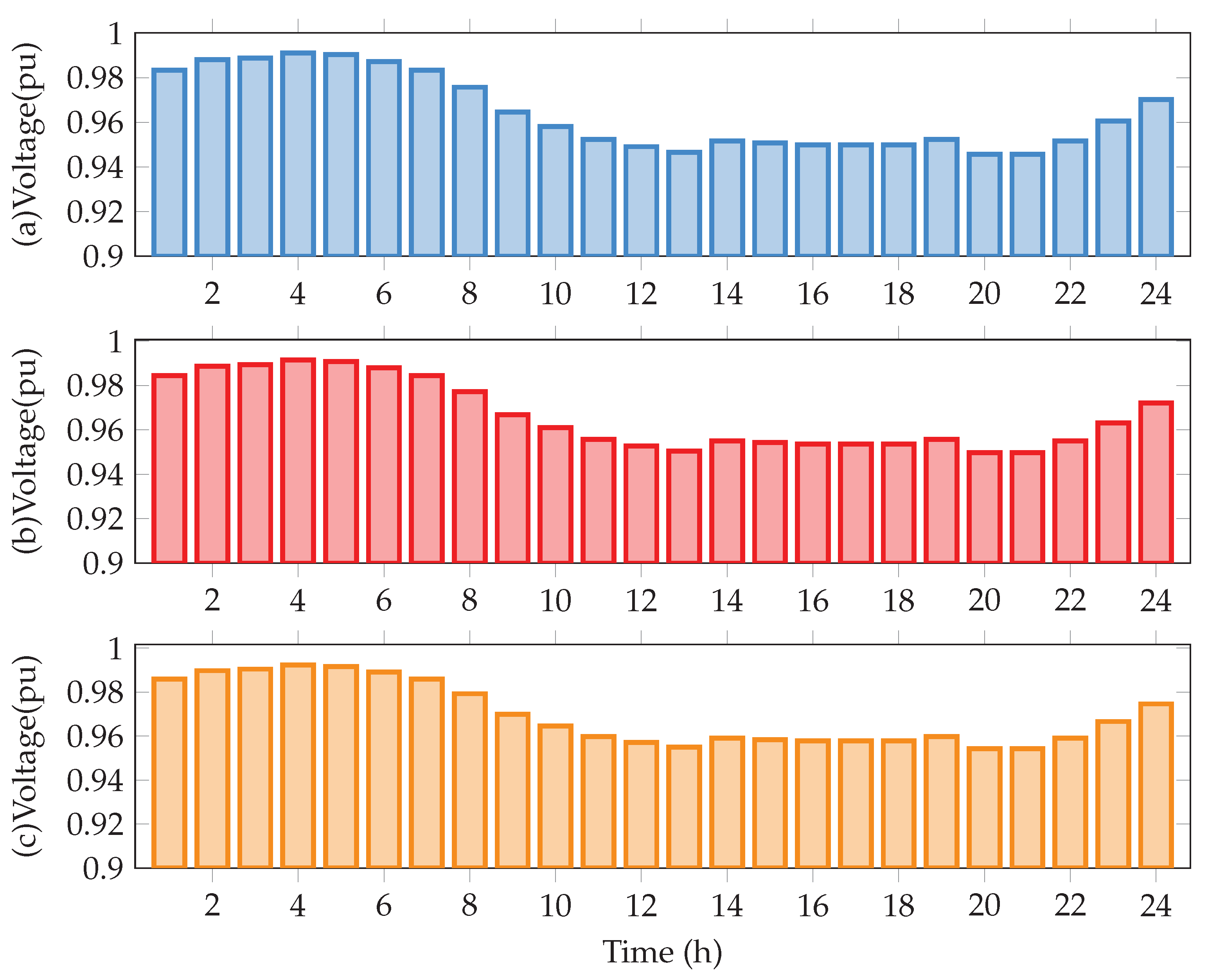
Regarding the voltage profiles, the minimum voltage during the period of peak demand was 0.9591 pu in phase A, 0.9463 pu in phase B, and 0.9689 pu in phase C in the 8-node test system and 0.9457 pu in phase A, 0.9498 pu in phase B, and 0.9543 pu in phase C in the 25-node test system. This demonstrates that the solution provided by the SSA respected the voltage regulation constraint established for the system, which was set at $\pm 10\%$.

Based on the conclusions drawn here, future studies could solve the problem under study using new metaheuristic methods with high numerical performance, such as the genetic algorithm, the vortex search algorithm, and the crow search algorithm. They could also consider using a multi-objective optimization approach that improves technical, economic, and environmental aspects while respecting the operating conditions of three-phase distribution systems. Finally, future research could include the problem of how to optimally integrate distributed generators based on renewable resources in the planning of three-phase distribution networks while considering the investment and maintenance costs of each distributed generator.

References

1. Löfquist, L. Is there a universal human right to electricity? Int. J. Hum. Rights 2020, 24, 711–723. [Google Scholar] [CrossRef]
2. Sarkodie, S.A.; Adams, S. Electricity access, human development index, governance and income inequality in Sub-Saharan Africa. Energy Rep. 2020, 6, 455–466. [Google Scholar] [CrossRef]
3. Ghiasi, M. Detailed study, multi-objective optimization, and design of an AC-DC smart microgrid with hybrid renewable energy resources. Energy 2019, 169, 496–507. [Google Scholar] [CrossRef]
4. Shen, T.; Li, Y.; Xiang, J. A Graph-Based Power Flow Method for Balanced Distribution Systems. Energies 2018, 11, 511. [Google Scholar] [CrossRef]
5. Ghiasi, M.; Niknam, T.; Dehghani, M.; Siano, P.; Alhelou, H.H.; Al-Hinai, A. Optimal Multi-Operation Energy Management in Smart Microgrids in the Presence of RESs Based on Multi-Objective Improved DE Algorithm: Cost-Emission Based Optimization. Appl. Sci. 2021, 11, 3661. [Google Scholar] [CrossRef]
6. Ouali, S.; Cherkaoui, A. An improved backward/forward sweep power flow method based on a new network information organization for radial distribution systems. J. Electr. Comput. Eng. 2020, 2020, 5643410. [Google Scholar] [CrossRef]
7. Aboshady, F.; Thomas, D.W.; Sumner, M. A wideband single end fault location scheme for active untransposed distribution systems. IEEE Trans. Smart Grid 2019, 11, 2115–2124. [Google Scholar] [CrossRef]
8. Arias, J.; Calle, M.; Turizo, D.; Guerrero, J.; Candelo-Becerra, J.E. Historical load balance in distribution systems using the branch and bound algorithm. Energies 2019, 12, 1219. [Google Scholar] [CrossRef]
9. Garcés-Ruiz, A. Power Flow in Unbalanced Three-Phase Power Distribution Networks Using Matlab: Theory, analysis, and quasi-dynamic simulation. Ingeniería 2022, 27, e19252. [Google Scholar] [CrossRef]
10. Cortés-Caicedo, B.; Avellaneda-Gómez, L.S.; Montoya, O.D.; Alvarado-Barrios, L.; Chamorro, H.R. Application of the Vortex Search Algorithm to the Phase-Balancing Problem in Distribution Systems. Energies 2021, 14, 1282. [Google Scholar] [CrossRef]
11. Cabrera, J.B.; Veiga, M.F.; Morales, D.X.; Medina, R. Reducing power losses in smart grids with cooperative game theory. In Advanced Communication and Control Methods for Future Smartgrids; Intechopen: London, UK, 2019; p. 49. [Google Scholar]
12. Trentini, C.; de Oliveira Guedes, W.; de Oliveira, L.W.; Dias, B.H.; Ferreira, V.H. Maintenance planning of electric distribution systems—A review. J. Control. Autom. Electr. Syst. 2021, 32, 186–202. [Google Scholar] [CrossRef]
13. Martínez-Gil, J.F.; Moyano-García, N.A.; Montoya, O.D.; Alarcon-Villamil, J.A. Optimal Selection of Conductors in Three-Phase Distribution Networks Using a Discrete Version of the Vortex Search Algorithm. Computation 2021, 9, 80. [Google Scholar] [CrossRef]
14. Wang, Z.; Liu, H.; Yu, D.C.; Wang, X.; Song, H. A practical approach to the conductor size selection in planning radial distribution systems. IEEE Trans. Power Deliv. 2000, 15, 350–354. [Google Scholar] [CrossRef]
15. Zhu, J.; Bilbro, G.; Chow, M.Y. Phase balancing using simulated annealing. IEEE Trans. Power Syst. 1999, 14, 1508–1513. [Google Scholar] [CrossRef]
16. Han, X.; Wang, H.; Liang, D. Master-slave game optimization method of smart energy systems considering the uncertainty of renewable energy. Int. J. Energy Res. 2021, 45, 642–660. [Google Scholar] [CrossRef]
17. Montoya, O.D.; Grajales, A.; Hincapié, R.A. Optimal Selection of Conductors in Distribution Systems Using Tabu Search Algorithm [Selección óptima de Conductores en Sistemas de Distribución Empleando el Algoritmo Búsqueda Tabú]. 2018. Available online: https://www.scielo.cl/scielo.php?script=sci_arttext&pid=S0718-33052018000200283&lng=en&nrm=iso (accessed on 3 July 2022).
18. Ismael, S.M.; Aleem, S.; Abdelaziz, A.Y. Optimal conductor selection in radial distribution systems using whale optimization algorithm. J. Eng. Sci. Technol. 2019, 14, 87–107. [Google Scholar]
19. Kumari, M.; Singh, V.; Ranjan, R. Optimal selection of conductor in RDS considering weather condition. In Proceedings of the 2018 International Conference on Computing, Power and Communication Technologies (GUCON), Greater Noida, India, 28–29 September 2018; pp. 647–651. [Google Scholar]
20. Mohanty, S.; Kasturi, K.; Nayak, M.R. Application of ER-WCA to Determine Conductor Size for Performance Improvement in Distribution System. In Proceedings of the 2021 International Conference on Advances in Electrical, Computing, Communication and Sustainable Technologies (ICAECT), Bhilai, India, 19–20 February 2021; pp. 1–5. [Google Scholar]
21. Montoya, O.D.; Serra, F.M.; De Angelo, C.H.; Chamorro, H.R.; Alvarado-Barrios, L. Heuristic Methodology for Planning AC Rural Medium-Voltage Distribution Grids. Energies 2021, 14, 5141. [Google Scholar] [CrossRef]
22. Garces, A.; Gil-González, W.; Montoya, O.D.; Chamorro, H.R.; Alvarado-Barrios, L. A Mixed-Integer Quadratic Formulation of the Phase-Balancing Problem in Residential Microgrids. Appl. Sci. 2021, 11, 1972. [Google Scholar] [CrossRef]
23. Cortés-Caicedo, B.; Avellaneda-Gómez, L.S.; Montoya, O.D.; Alvarado-Barrios, L.; Álvarez-Arroyo, C. An improved crow search algorithm applied to the phase swapping problem in asymmetric distribution systems. Symmetry 2021, 13, 1329. [Google Scholar] [CrossRef]
24. Cruz-Reyes, J.L.; Salcedo-Marcelo, S.S.; Montoya, O.D. Application of the Hurricane-Based Optimization Algorithm to the Phase-Balancing Problem in Three-Phase Asymmetric Networks. Computers 2022, 11, 43. [Google Scholar] [CrossRef]
25. Montoya, O.D.; Molina-Cabrera, A.; Grisales-Noreña, L.F.; Hincapié, R.A.; Granada, M. Improved genetic algorithm for phase-balancing in three-phase distribution networks: A master-slave optimization approach. Computation 2021, 9, 67. [Google Scholar] [CrossRef]
26. Montoya, O.D.; Alarcon-Villamil, J.A.; Hernández, J.C. Operating cost reduction in distribution networks based on the optimal phase-swapping including the costs of the working groups and energy losses. Energies 2021, 14, 4535. [Google Scholar] [CrossRef]
27. Mandal, S.; Pahwa, A. Optimal selection of conductors for distribution feeders. IEEE Trans. Power Syst. 2002, 17, 192–197. [Google Scholar] [CrossRef]
28. Joshi, D.; Burada, S.; Mistry, K.D. Distribution system planning with optimal conductor selection. In Proceedings of the 2017 Recent Developments in Control, Automation & Power Engineering (RDCAPE), Noida, India, 26–27 October 2017; pp. 263–268. [Google Scholar]
29. Rao, R.S.; Satish, K.; Narasimham, S. Optimal conductor size selection in distribution systems using the harmony search algorithm with a differential operator. Electr. Power Compon. Syst. 2011, 40, 41–56. [Google Scholar] [CrossRef]
30. López, L.; Hincapié, R.A.; Gallego, R.A. Multi-objective Distribution System Planning using an NSGA II Evolutionary Algorithm [Planeamiento multiobjetivo de sistemas de distribución usando un algoritmo evolutivo NSGA-II]. Rev. EIA 2011, 8, 141–151. Available online: https://revistas.eia.edu.co/index.php/reveia/article/view/252 (accessed on 9 November 2021).
31. Khalil, T.M.; Gorpinich, A.V. Optimal conductor selection and capacitor placement for loss reduction of radial distribution systems by selective particle swarm optimization. In Proceedings of the 2012 Seventh International Conference on Computer Engineering & Systems (ICCES), Cairo, Egypt, 27–29 September 2012; pp. 215–220. [Google Scholar]
32. Legha, M.M.; Javaheri, H.; Legha, M.M. Optimal Conductor Selection in Radial Distribution Systems for Productivity Improvement Using Genetic Algorithm. Iraqi J. Electr. Electron. Eng. 2013, 9, 29–35. [Google Scholar] [CrossRef]
33. Legha, M.M.; Noormohamadi, H.; Barkhori, A. Optimal conductor selection in radial distribution using bacterial foraging algorithm and comparison with ICA method. WALIA J. 2015, 31, 37–43. [Google Scholar]
34. Ismael, S.M.; Aleem, S.H.A.; Abdelaziz, A.Y. Optimal selection of conductors in Egyptian radial distribution systems using sine-cosine optimization algorithm. In Proceedings of the 2017 Nineteenth International Middle East Power Systems Conference (MEPCON), Cairo, Egypt, 19–21 September 2017; pp. 103–107. [Google Scholar]
35. Abdelaziz, A.Y.; Fathy, A. A novel approach based on crow search algorithm for optimal selection of conductor size in radial distribution networks. Eng. Sci. Technol. Int. J. 2017, 20, 391–402. [Google Scholar] [CrossRef]
36. Montoya, O.D.; Gil-González, W.; Grisales-Norena, L.F. On the mathematical modeling for optimal selecting of calibers of conductors in DC radial distribution networks: An MINLP approach. Electr. Power Syst. Res. 2021, 194, 107072. [Google Scholar] [CrossRef]
37. Chen, T.H.; Cherng, J.T. Optimal phase arrangement of distribution transformers connected to a primary feeder for system unbalance improvement and loss reduction using a genetic algorithm. In Proceedings of the 21st International Conference on Power Industry Computer Applications. Connecting Utilities. PICA 99. To the Millennium and Beyond (Cat. No. 99CH36351), Santa Clara, CA, USA, 21 May 1999; pp. 145–151. [Google Scholar]
38. Gandomkar, M. Phase balancing using genetic algorithm. In Proceedings of the 39th International Universities Power Engineering Conference (UPEC 2004), Bristol, UK, 6–8 September 2004; Volume 1, pp. 377–379. [Google Scholar]
39. Granada Echeverri, M.; Gallego Rendón, R.A.; López Lezama, J.M. Optimal phase balancing planning for loss reduction in distribution systems using a specialized genetic algorithm. Ing. Cienc. 2012, 8, 121–140. [Google Scholar] [CrossRef]
40. Rios, M.A.; Castano, J.C.; Garcés, A.; Molina-Cabrera, A. Phase Balancing in Power Distribution Systems: A heuristic approach based on group-theory. In Proceedings of the 2019 IEEE Milan PowerTech, Milan, Italy, 23–27 June 2019; pp. 1–6. [Google Scholar]
41. Garcés-Ruiz, A.; Granada-Echeverri, M.; Gallego, R.A. Balance de fases usando colonia de hormigas. Ing. Compet. 2005, 7, 43–52. [Google Scholar] [CrossRef]
42. Tuppadung, Y.; Kurutach, W. The modified particle swarm optimization for phase balancing. In Proceedings of the TENCON 2006-2006 IEEE Region 10 Conference, Hong Kong, China, 14–17 November 2006; pp. 1–4. [Google Scholar]
43. Toma, N.; Ivanov, O.; Neagu, B.; Gavrila, M. A PSO algorithm for phase load balancing in low voltage distribution networks. In Proceedings of the 2018 International Conference and Exposition on Electrical And Power Engineering (EPE), Iasi, Romania, 18–19 October 2018; pp. 0857–0862. [Google Scholar]
44. Huang, M.Y.; Chen, C.S.; Lin, C.H.; Kang, M.S.; Chuang, H.J.; Huang, C.W. Three-phase balancing of distribution feeders using immune algorithm. IET Gener. Transm. Distrib. 2008, 2, 383–392. [Google Scholar] [CrossRef]
45. Sathiskumar, M.; Lakshminarasimman, L.; Thiruvenkadam, S. A self adaptive hybrid differential evolution algorithm for phase balancing of unbalanced distribution system. Int. J. Electr. Power Energy Syst. 2012, 42, 91–97. [Google Scholar] [CrossRef]
46. Hooshmand, R.; Soltani, S. Simultaneous optimization of phase balancing and reconfiguration in distribution networks using BF–NM algorithm. Int. J. Electr. Power Energy Syst. 2012, 41, 76–86. [Google Scholar] [CrossRef]
47. Montoya, O.D.; Arias-Londoño, A.; Grisales-Noreña, L.F.; Barrios, J.Á.; Chamorro, H.R. Optimal Demand Reconfiguration in Three-Phase Distribution Grids Using an MI-Convex Model. Symmetry 2021, 13, 1124. [Google Scholar] [CrossRef]
48. Montoya, O.D.; Grisales-Noreña, L.F.; Rivas-Trujillo, E. Approximated Mixed-Integer Convex Model for Phase Balancing in Three-Phase Electric Networks. Computers 2021, 10, 109. [Google Scholar] [CrossRef]
49. Hu, R.; Li, Q.; Qiu, F. Ensemble learning based convex approximation of three-phase power flow. IEEE Trans. Power Syst. 2021, 36, 4042–4051. [Google Scholar] [CrossRef]
50. Carreno, I.L.; Scaglione, A.; Saha, S.S.; Arnold, D.; Ngo, S.T.; Roberts, C. Log (v) 3LPF: A Linear Power Flow Formulation for Unbalanced Three-Phase Distribution Systems. IEEE Trans. Power Syst. 2022. [Google Scholar] [CrossRef]
51. Lavorato, M.; Franco, J.F.; Rider, M.J.; Romero, R. Imposing radiality constraints in distribution system optimization problems. IEEE Trans. Power Syst. 2011, 27, 172–180. [Google Scholar] [CrossRef]
52. Devikanniga, D.; Vetrivel, K.; Badrinath, N. Review of meta-heuristic optimization based artificial neural networks and its applications. J. Phys. Conf. Ser. 2019, 1362, 012074. [Google Scholar] [CrossRef]
53. Mirjalili, S.; Gandomi, A.H.; Mirjalili, S.Z.; Saremi, S.; Faris, H.; Mirjalili, S.M. Salp Swarm Algorithm: A bio-inspired optimizer for engineering design problems. Adv. Eng. Softw. 2017, 114, 163–191. [Google Scholar] [CrossRef]
54. Salimon, S.A.; Aderinko, H.A.; Fajuke, F.; Suuti, K.A. Load flow analysis of nigerian radial distribution network using backward/forward sweep technique. J. VLSI Des. Adv. 2019, 2, 1–11. [Google Scholar] [CrossRef]
55. Jabari, F.; Sohrabi, F.; Pourghasem, P.; Mohammadi-Ivatloo, B. Backward-forward sweep based power flow algorithm in distribution systems. In Optimization of Power System Problems; Springer: Berlin/Heidelberg, Germany, 2020; pp. 365–382. [Google Scholar]
56. Hegazy, A.E.; Makhlouf, M.; El-Tawel, G.S. Improved salp swarm algorithm for feature selection. J. King Saud Univ.-Comput. Inf. Sci. 2020, 32, 335–344. [Google Scholar] [CrossRef]
57. Abualigah, L.; Shehab, M.; Alshinwan, M.; Alabool, H. Salp swarm algorithm: A comprehensive survey. Neural Comput. Appl. 2020, 32, 11195–11215. [Google Scholar] [CrossRef]
58. Ibrahim, R.A.; Ewees, A.A.; Oliva, D.; Abd Elaziz, M.; Lu, S. Improved salp swarm algorithm based on particle swarm optimization for feature selection. J. Ambient. Intell. Humaniz. Comput. 2019, 10, 3155–3169. [Google Scholar] [CrossRef]
59. Zhang, H.; Liu, T.; Ye, X.; Heidari, A.A.; Liang, G.; Chen, H.; Pan, Z. Differential evolution-assisted salp swarm algorithm with chaotic structure for real-world problems. Eng. Comput. 2022. [Google Scholar] [CrossRef]
60. Adetunji, K.E.; Hofsajer, I.W.; Abu-Mahfouz, A.M.; Cheng, L. A review of metaheuristic techniques for optimal integration of electrical units in distribution networks. IEEE Access 2020, 9, 5046–5068. [Google Scholar] [CrossRef]
61. Faris, H.; Mirjalili, S.; Aljarah, I.; Mafarja, M.; Heidari, A.A. Salp swarm algorithm: Theory, literature review, and application in extreme learning machines. Nat.-Inspir. Optim. 2020, 811, 185–199. [Google Scholar] [CrossRef]
62. Castelli, M.; Manzoni, L.; Mariot, L.; Nobile, M.S.; Tangherloni, A. Salp Swarm Optimization: A critical review. Expert Syst. Appl. 2022, 189, 116029. [Google Scholar] [CrossRef]
63. Montano, J.; Mejia, A.F.T.; Rosales Muñoz, A.A.; Andrade, F.; Garzon Rivera, O.D.; Palomeque, J.M. Salp Swarm Optimization Algorithm for Estimating the Parameters of Photovoltaic Panels Based on the Three-Diode Model. Electronics 2021, 10, 3123. [Google Scholar] [CrossRef]
64. Asl, D.K.; Seifi, A.R.; Rastegar, M.; Mohammadi, M. Optimal energy flow in integrated energy distribution systems considering unbalanced operation of power distribution systems. Int. J. Electr. Power Energy Syst. 2020, 121, 106132. [Google Scholar]
65. Pandey, A.; Jereminov, M.; Wagner, M.R.; Bromberg, D.M.; Hug, G.; Pileggi, L. Robust power flow and three-phase power flow analyses. IEEE Trans. Power Syst. 2018, 34, 616–626. [Google Scholar] [CrossRef]
66. Kersting, W.H. Distribution System Modeling and Analysis; CRC Press: Boca Raton, FL, USA, 2006. [Google Scholar]
67. Souza, B.; Araujo, L.; Penido, D. An Extended Kron Method for Power System Applications. IEEE Lat. Am. Trans. 2020, 18, 1470–1477. [Google Scholar] [CrossRef]
68. Kersting, W.H. Radial distribution test feeders. IEEE Trans. Power Syst. 1991, 6, 975–985. [Google Scholar] [CrossRef]
69. Mwakabuta, N.; Sekar, A. Comparative study of the IEEE 34 node test feeder under practical simplifications. In Proceedings of the 2007 39th North American Power Symposium, Las Cruces, NM, USA, 30 September–2 October 2007; pp. 484–491. [Google Scholar]
70. Montoya, O.D.; Giraldo, J.S.; Grisales-Noreña, L.F.; Chamorro, H.R.; Alvarado-Barrios, L. Accurate and Efficient Derivative-Free Three-Phase Power Flow Method for Unbalanced Distribution Networks. Computation 2021, 9, 61. [Google Scholar] [CrossRef]
71. Gil-González, W.; Montoya, O.D.; Grisales-Noreña, L.F.; Perea-Moreno, A.J.; Hernandez-Escobedo, Q. Optimal placement and sizing of wind generators in AC grids considering reactive power capability and wind speed curves. Sustainability 2020, 12, 2983. [Google Scholar] [CrossRef]
72. Montoya, O.D.; Gil-González, W.; Giral, D.A. On the Matricial Formulation of Iterative Sweep Power Flow for Radial and Meshed Distribution Networks with Guarantee of Convergence. Appl. Sci. 2020, 10, 5802. [Google Scholar] [CrossRef]
73. Sahoo, R.R.; Ray, M. PSO based test case generation for critical path using improved combined fitness function. J. King Saud-Univ.-Comput. Inf. Sci. 2020, 32, 479–490. [Google Scholar] [CrossRef]
74. Zhang, X.; Beram, S.M.; Haq, M.A.; Wawale, S.G.; Buttar, A.M. Research on algorithms for control design of human–machine interface system using ML. Int. J. Syst. Assur. Eng. Manag. 2022, 13, 462–469. [Google Scholar] [CrossRef]
75. Harman, M.; Jia, Y.; Zhang, Y. Achievements, open problems and challenges for search based software testing. In Proceedings of the 2015 IEEE 8th International Conference on Software Testing, Verification and Validation (ICST), Graz, Austria, 13–17 April 2015; pp. 1–12. [Google Scholar]
76. Enel Codensa, S.A. LA202 Circuito Primario Sencillo Construcción Tangencial, Bogotá, Colombia. Available online: https://likinormas.micodensa.com/Norma/lineas_aereas_urbanas_distribucion/lineas_aereas_11_4_13_2_kv/la202_circuito_primario_sencillo_construccion_tangencial (accessed on 5 May 2022).
77. Enel Codensa, S.A. LA006 Distancias de Construcción Para Circuitos de 13,2 -11,4 kv Y B.T., Bogotá, Colombia. Available online: https://likinormas.micodensa.com/Norma/lineas_aereas_urbanas_distribucion/la006_distancias_construccion_circuitos_13_2_11 (accessed on 5 May 2022).
78. Gil-González, W.; Montoya, O.D.; Holguín, E.; Garces, A.; Grisales-Noreña, L.F. Economic dispatch of energy storage systems in dc microgrids employing a semidefinite programming model. J. Energy Storage 2019, 21, 1–8. [Google Scholar] [CrossRef]
79. Montoya, O.D.; Gil-González, W.; Grisales-Noreña, L.; Orozco-Henao, C.; Serra, F. Economic dispatch of BESS and renewable generators in DC microgrids using voltage-dependent load models. Energies 2019, 12, 4494. [Google Scholar] [CrossRef] [Green Version]
80. Comisión de Regulación de Energía y Gas. Resolución 025 de 1995, Bogotá, Colombia. 1995. Available online: http://apolo.creg.gov.co/Publicac.nsf/Indice01/Resoluci%C3%B3n-1995-CRG95025 (accessed on 5 May 2022).
Figure 1. Network segment of a three-phase distribution system.
Mathematics 10 03327 g001
Figure 2. IEEE ID-500 overhead distribution line.
Mathematics 10 03327 g002
Figure 3. Electrical configuration of the 8-node test system.
Mathematics 10 03327 g003
Figure 4. Electrical configuration of the 25-node test system.
Mathematics 10 03327 g004
Figure 5. LA202 overhead distribution line.
Mathematics 10 03327 g005
Figure 6. Typical behavior of a demand curve in Colombia over a 24-h period.
Mathematics 10 03327 g006
Figure 7. Average unbalance percentage over a one-day operation in the 8-node system.
Mathematics 10 03327 g007
Figure 8. Behavior of the current magnitude at the main feeder in the 8-node test system over a one-day operation.
Mathematics 10 03327 g008
Figure 9. Behavior of the minimum voltage magnitude in the 8-node test system over a one-day operation: (a) phase A, (b) phase B, and (c) phase C.
Mathematics 10 03327 g009
Figure 10. Average unbalance percentage over a one-day operation in the 25-node system.
Mathematics 10 03327 g010
Figure 11. Behavior of the current magnitude at the main feeder in the 25-node test system over a one-day operation.
Mathematics 10 03327 g011
Figure 12. Behavior of the minimum voltage magnitude in the 25-node test system over a one-day operation: (a) phase A, (b) phase B, and (c) phase C.
Mathematics 10 03327 g012