Runge–Kutta Embedded Methods of Orders 8(7) for Use in Quadruple Precision Computations

Abstract

High algebraic order Runge–Kutta embedded methods are commonly used when stringent tolerances are demanded. Traditionally, various criteria are satisfied while constructing these methods for application in double precision arithmetic. Firstly we try to keep the magnitude of the coefficients low, otherwise we may experience loss of accuracy; however, when working in quadruple precision we may admit larger coefficients. Then we are able to construct embedded methods of orders eight and seven (i.e., pairs of methods) with even smaller truncation errors. A new derived pair, as expected, is performing better than state-of-the-art pairs in a set of relevant problems.

1. Introduction

The initial value problem (IVP) of the first order has the following form

$${\zeta }^{\prime }=f(x,\zeta ),\zeta \left(x_0\right)={\zeta }_0\in {\mathbb{R}}^m,x\in [x_0,x_e],$$

(1)

with $f:\mathbb{R}\times {\mathbb{R}}^m\to {\mathbb{R}}^m$ continuously differentiable.

Among the typical numerical approaches for addressing (1) are RK embedded methods, which are defined by the extended Butcher tableau [1,2] shown below

$$\begin{array}{c}\begin{array}{cc}c& A\end{array}\\ \begin{array}{cc} \hspace{0.17em}& w\\ \hspace{0.17em}& \widehat{w}\end{array}\end{array}$$

where $A\in {\mathbb{R}}^{s\times s}$ with $a_{ij}=0,i\le j$ and $w^T$, ${\widehat{w}}^T$, $c\in {\mathbb{R}}^s$. This is an $s$—stage RK pair and the numerical approximation of the solution advances from $(x_n,{\zeta }_n)$ to $x_{n+1}=x_n+h_n$ after evaluating at each step two approximations ${\zeta }_{n+1}$, ${\widehat{\zeta }}_{n+1}$ to $\zeta \left(t_{n+1}\right)$ of orders p and q (with $q<p$), respectively, given by

$${\zeta }_{n+1}={\zeta }_n+h_n\sum _{i=1}^s{w}_i{f}_{ni}$$

and

$${\widehat{\zeta }}_{n+1}={\zeta }_n+h_n\sum _{i=1}^s{\widehat{w}}_i{f}_{ni},$$

with

$$f_{ni}=f(x_n+c_i{h}_n,{\zeta }_n+h_n\sum _{j=1}^{i-1}{a}_{ij}{f}_{nj}),$$

for $i=1$, $2,...,s\ge p$.

The local error made is estimated in every step by [3]

$${ϵ}_{n+1}=∥{\zeta }_{n+1}-{\widehat{\zeta }}_{n+1}∥·h^{p-q+1}.$$

The above is used in order to change the step according to

$$h_{n+1}=0.9·h_n·{\left(\frac{\epsilon }{{ϵ}_{n+1}}\right)}^{1/p},$$

where the user sets a very small positive tolerance $\epsilon$, valid through the whole integration. In case that $\epsilon <{ϵ}_{n+1}$, we also use this formula but then we may accept $h_n=h_{n+1}$ as the new decreased length of $h_n$. More details in the subject can be retrieved from [3].

2. Runge–Kutta Pairs of Orders Eight and Seven

If the coefficient parameters in A, w, $\widehat{w}$, and c fulfill certain algebraic criteria, an RK pair of order $p\left(q\right)$ is formed. A set of nonlinear equations describes these conditions. This system’s general (parametric) solution is known only for orders up to five. However, no practical application has been discovered for Cassity’s fifth-order families of approaches discussed in [4]. Only specific families of this system’s general solution are known for higher order approaches.The more free nodes $c_i$, $i=2$, $3,\cdots ,s$ there are, the easier it is to locate individual pairings of these families that meet specific design requirements. These nonstiff problem criteria are concerned with the reduction in certain truncation error coefficients measure, and for mildly stiff issues with maximizing the stability region.

Since (1) is a system, we may embed independent variable x in $\zeta$ and consider only autonomous systems ${\zeta }^{\prime }=f\left(\zeta \right)$. When used to an autonomous system of differential equations, a Runge–Kutta method is said to be of algebraic order p if and only if

$$\mathsf{\Psi }\left(\tau \right)=0\mathrm{for}\mathrm{every}\tau \in T_i,\mathrm{for}i=1\left(1\right)p$$

(2)

where $T_i$ is the set of i-th order (rooted) trees and

$$\mathsf{\Psi }\left(\tau \right)=\frac{1}{\sigma \left(\tau \right)}\left(X\left(\tau \right)-\frac{1}{\gamma \left(\tau \right)}\right).$$

$\sigma$, $\gamma$ are integral functions of $\tau$ (symmetry and density function, respectively, in the terminology introduced by Butcher [5]) and X is a certain composition of A, w, c (in case of the lower order formula replace with $\widehat{w}$). In the following the symbol $T^{\left(i\right)}$ denotes a vector with elements all the elements of the set $\mathsf{\Psi }\left(T_i\right)$ in some arbitrary order.

In the case of a $8\left(7\right)$ pair, Equation (2) is expanded in 200 nonlinear algebraic equations that must be satisfied by its higher order method and another 85 equations by its lower order method as shown in

Table 1. Number of order conditions for order p.

p	1	2	3	4	5	6	7	8	9	10
length of $T^{\left(i\right)}$	1	1	2	4	9	20	48	115	286	719

. For a list of these equations see for example Fehlberg [6]. A more comprehensive study with symbolic code for fast derivation of the equations of condition is given in [7]. The simplifying assumption

$$A·e=c,e={\left[1,1,1,\dots ,1,1\right]}^T\in {\mathbb{R}}^s,$$

(3)

is fulfilled in every RK method with perhaps the only exception being the Runge–Kutta–Oliver methods introduced in [8] and studied further in [9].

The minimal number of stages required for the construction of a $8\left(7\right)$ pair is 13 (i.e., hereafter $s=13$) and such a method offers only 104 parameters in view of (3). Because the number of unknowns is much fewer than the number of equations, and especially because some of the latter equations are significantly nonlinear with respect to the components of A, certain simplifying assumptions must be used to their solution.

Fehlberg was the first to construct such a pair; his pair has the disadvantage of producing identically zero error estimates for quadrature situations ${\zeta }^{\prime }=f\left(x\right)$ in Equation (1). This defect comes after the seventh-order formula satisfies the eighth-order condition $\widehat{b}·c^7=\frac{1}{8}$.

In the following, whenever c is a vector, we represent componentwise multiplication by

$$c^i=\underset{i}{\underbrace{c\circ c\circ \cdots \circ c}}$$

(assuming $c^0=e$). For this multiplication (called Hadamard multiplication) we admit lower order of precedence over the conventional dot product. We define $C=\mathrm{diag}\left(c\right)$ and we use the notation $c_{\left(j+\right)}$ for vector c but with its first $\left(j-1\right)$ elements dropped. Accordingly, we use the notation $c_{\left(i,j\right)}$ for the vector containing the elements of c beginning from index i through j. When applying these notations to a relation, it is assumed that it applies to both sides. See [10] for details in the issues described in this paragraph.

Various authors derived RK8(7) pairs after Fehlberg avoiding the quadrature defect; in chronological order, Verner [11], Prince and Dormand [12], Papakostas [13], Papakostas and Tsitouras [3,14], and Verner [15,16,17]. These pairs generally obey the following simplifying assumptions

$${\left(A·c=\frac{c^2}{2}\right)}_{\left(3+\right)},{\left(A·c^2=\frac{c^3}{3}\right)}_{\left(3+\right)},{\left(A·c^3=\frac{c^4}{4}\right)}_{\left(6+\right)}.$$

We additionally employ

$$w·\left(A+C-I_s\right)=0_s,\widehat{w}·\left(A+C-I_s\right)=0_s$$

with $I_s\in {\mathbb{R}}^{s\times s}$ the identity matrix and $0_s\in {\mathbb{R}}^s$ the vector with zero components.

Then we experience a severe reduction in the number of equations to be satisfied. In addition some elementary subsidiary equations can be solved instead—see the algorithm below for details.

The authors mentioned above gave some general lines of how to construct various types of embedded methods in a range of orders. A straightforward and explicit algorithm for the derivation of embedded methods of orders eight and seven is presented below.

Thus, we firstly set

$$w_2=w_3=w_4=w_5=0,{\widehat{w}}_2={\widehat{w}}_3={\widehat{w}}_4={\widehat{w}}_5=0,c_{12}=c_{13}=1,$$

$$a_{13,12}=0,a_{j2}=0,j=4,5,\cdots ,13,\mathrm{and}{a}_{j3}=0,j=6,7,\cdots ,13.$$

Then we choose arbitrarily the coefficients

$$c_2,c_5,c_6,c_7,c_8,c_{10},c_{11},a_{87},{\widehat{w}}_{12},{\widehat{w}}_{13},w_{13},$$

with the nodes being distinct from each other and at least one of ${\widehat{w}}_{13},w_{13}$ different from zero. The rest coefficients are found successively by the algorithm given below.

• Set

  $$c_9=\frac{1}{2}·\frac{\left\{\begin{array}{c}14c_6^2(7c_7^2{c}_8+c_7(7c_8^2-12c_8+1)+c_8)\\ +c_6(14c_7^2(7c_8^2-12c_8+1)-7c_7(24c_8^2-33c_8+4)+14c_8^2-28c_8+3)\\ +14c_7^2{c}_8+c_7(14c_8^2-28c_8+3)+3c_8\end{array}\right\}}{\left\{\begin{array}{c}7c_6^2(7c_7^2(15c_8^2-10c_8+2)-2c_7(35c_8^2-26c_8+6)+14c_8^2-12c_8+3)\\ -7c_6(2c_7^2(35c_8^2-26c_8+6)-c_7(52c_8^2-42c_8+11)+12c_8^2-11c_8+3)\\ +7c_7^2(14c_8^2-12c_8+3)-7c_7(12c_8^2-11c_8+3)+21c_8^2-21c_8+6\end{array}\right\}}$$
• Set $c_4=c_6(4c_5-3c_6)/\left(2(3c_5-2c_6)\right),c_3=2c_4/3,a_{32}=c_3^2/\left(2c_2\right),a_{43}=c_4^2/\left(2c_3\right),a_{54}=c_5^2(3c_3-2c_5)/\left(6c_4(c_3-c_4)\right)$
• Solve $w·c^i=\frac{1}{i+1},i=1,2,\cdots ,7$, for $w_1,w_6,\cdots ,w_{12}$.
• Solve $\widehat{w}·c^i=\frac{1}{i+1},i=1,2,\cdots ,6$, for ${\widehat{w}}_1,{\widehat{w}}_6,\cdots ,{\widehat{w}}_{12}$.

Then all the remaining coefficients of matrix A are linearly depended on the following 56 equations and can be derived by solving directly the corresponding linear system.

• Solve ${(w·(C-I_s)·A=0_s)}_{(4-5)}$, ${(w·{(C-I_s)}^2·A=0_s)}_{(4-5)}$, ${\left(A·c=\frac{c^2}{2}\right)}_{(5-12)}$,
  ${\left(A·c^2=\frac{c^3}{3}\right)}_{(5-12)}$, ${\left(A·c^3=\frac{c^4}{4}\right)}_{(7-12)}$, ${\left(w·\left(A+C-I_s\right)=0_s\right)}_{(4-10)}$,
  ${\left(\widehat{w}·\left(A+C-I_s\right)=0_s\right)}_{(4-8)}$, ${(\widehat{w}·(C-I_s)·A)}_4=0$, $w·(c\circ (A·c^4))=\frac{1}{35}$,
  $w·(c^2\circ (A·c^4))=\frac{1}{40}$, $w·(c\circ (A·c^5))=\frac{1}{48}$, $\widehat{w}·(c\circ (A·c^4))=\frac{1}{35}$, ${(A·e=c)}_{(2-13)}$ for the remaining coefficients from matrix A.

Next we provide a Mathematica package that implements the algorithm above. The following listing is 100% error free and is copied directly from the actual file.

(*----------------------------------------------------------------------------------------*)

BeginPackage["T87‘"];

Clear["T87‘*"];

 

T87::usage="T87[c2,c5,c6,c7,c8,c10,c11,a87,w13,ww12,ww13]

        returns the coefficients matrices a,w,ww,c

        of RK embedded pair of orders 8(7)"

 

Begin["‘Private‘"];

Clear["T87‘Private‘*"];

 

 

T87[c2_,c5_,c6_,c7_,c8_,c10_,c11_,a87_,w13_,ww12_,ww13_]:=

Module[  {c, c3, c4, c9, w, ww, e, a, w1, w6, w7, w8, w9, w10, w11, w12, ww1, ww6, ww7, ww8,

  ww9, ww10, ww11, ae, ac, ac2, ac3, cc, ii, baci, bbaci, a32, a43, a53, a54, a64, a65, a74,

 a75, a76, a84, a85, a86, a94, a95, a96, a97, a98, a104, a105, a106, a107, a108, a109, a114,

a115, a116, a117, a118, a119, a1110, a124, a125, a126, a127, a128, a129, a1210, a1211, a134,

   a135, a136, a137, a138, a139, a1310, a1311, a21, a31, a41, a51, a61, a71, a81, a91, a101,

                                             a111, a121, a131},

c = {0, c2, c3, c4, c5, c6, c7, c8, c9, c10, c11, 1, 1};

w = {w1, 0, 0, 0, 0, w6, w7, w8, w9, w10, w11, w12, w13};

ww = {ww1, 0, 0, 0, 0, ww6, ww7, ww8, ww9, ww10, ww11, ww12, ww13};

e = {1, 1, 1, 1, 1, 1, 1, 1, 1, 1, 1, 1, 1};

a = {{0, 0, 0, 0, 0, 0, 0, 0, 0, 0, 0, 0, 0},

    {a21, 0, 0, 0, 0, 0, 0, 0, 0, 0, 0, 0, 0},

    {a31, a32, 0, 0, 0, 0, 0, 0, 0, 0, 0, 0, 0},

    {a41, 0, a43, 0, 0, 0, 0, 0, 0, 0, 0, 0, 0},

    {a51, 0, a53, a54, 0, 0, 0, 0, 0, 0, 0, 0, 0},

    {a61, 0, 0, a64, a65, 0, 0, 0, 0, 0, 0, 0, 0},

    {a71, 0, 0, a74, a75, a76, 0, 0, 0, 0, 0, 0, 0},

    {a81, 0, 0, a84, a85, a86, a87, 0, 0, 0, 0, 0, 0},

    {a91, 0, 0, a94, a95, a96, a97, a98, 0, 0, 0, 0, 0},

    {a101, 0, 0, a104, a105, a106, a107, a108, a109, 0, 0, 0, 0},

    {a111, 0, 0, a114, a115, a116, a117, a118, a119, a1110, 0, 0, 0},

    {a121, 0, 0, a124, a125, a126, a127, a128, a129, a1210, a1211, 0, 0},

    {a131, 0, 0, a134, a135, a136, a137, a138, a139, a1310, a1311, 0, 0}};

c9 = (14*c6^2*(7*c7^2*c8 + c7*(7*c8^2 - 12*c8 + 1) + c8) + c6*(14*c7^2*(7*c8^2 - 12*c8 + 1)

    - 7*c7*(24*c8^2 - 33*c8 + 4) + 14*c8^2 - 28*c8 + 3) + 14*c7^2*c8

    + c7*(14*c8^2 - 28*c8 + 3) + 3*c8)/

    (2*(7*c6^2*(7*c7^2*(15*c8^2 - 10*c8 + 2) - 2*c7*(35*c8^2 - 26*c8 + 6)

     + 14*c8^2 - 12*c8 + 3) - 7*c6*(2*c7^2*(35*c8^2 - 26*c8 + 6)

     - c7*(52*c8^2 - 42*c8 + 11) + 12*c8^2 - 11*c8 + 3) + 7*c7^2*(14*c8^2 - 12*c8 + 3)

     - 7*c7*(12*c8^2 - 11*c8 + 3) + 21*c8^2 - 21*c8 + 6));

c3 = (3*c2)/2; c4 = (9*c2)/4; a32 = (9*c2)/8; a43 = (27*c2)/16;

{w1, w6, w7, w8, w9, w10, w11, w12} =

             Solve[{w.e == 1, w.c == 1/2, w.c^2 == 1/3, w.c^3 == 1/4, w.c^4 == 1/5,

                              w.c^5 == 1/6, w.c^6 == 1/7, w.c^7 == 1/8},

                         {w1, w6, w7, w8, w9, w10, w11, w12}][[1, All, 2]];

{ww1, ww6, ww7, ww8, ww9, ww10, ww11} =

Solve[{ww.e == 1, ww.c == 1/2, ww.c^2 == 1/3, ww.c^3 == 1/4, ww.c^4 == 1/5,

                           ww.c^5 == 1/6, ww.c^6 == 1/7},

                        {ww1, ww6, ww7, ww8, ww9, ww10, ww11}][[1, All, 2]];

ae = a.e - c; ac = a.c - c^2/2; ac2 = a.c^2 - c^3/3; ac3 = a.c^3 - c^4/4;

cc = DiagonalMatrix[c]; ii = IdentityMatrix[13];

baci = w.(a + cc - ii); bbaci = ww.(a + cc - ii);

{a53, a54, a64, a65, a74, a75, a76, a84, a85, a86, a94, a95, a96, a97, a98, a104, a105,

 a106, a107, a108, a109, a114, a115, a116, a117, a118, a119, a1110, a124, a125, a126, a127,

         a128, a129, a1210, a1211, a134, a135, a136, a137, a138, a139, a1310, a1311} =

 Solve[ Join[(w.(cc - ii).a)[[4 ;; 5]], (w.(cc - ii).(cc - ii).a)[[4 ;; 5]], ac[[5 ;; 12]],

               ac2[[5 ;; 12]], ac3[[7 ;; 13]], baci[[4 ;; 10]], bbaci[[4 ;; 8]],

            {(ww.(cc - ii).a)[[4]], -(1/35) + w.(c a.c^4), -(1/40) + w.(c^2 a.c^4),

               -(1/48) + w.(c a.c^5), -(1/35) + ww.(c a.c^4)}] == Array[0 &, 44],

    {a53, a54, a64, a65, a74, a75, a76, a84, a85, a86, a94, a95, a96, a97, a98, a104, a105,

 a106, a107, a108, a109, a114, a115, a116, a117, a118, a119, a1110, a124, a125, a126, a127,

 a128, a129, a1210, a1211, a134, a135, a136, a137, a138, a139, a1310, a1311}][[1, All, 2]];

{a21, a31, a41, a51, a61, a71, a81, a91, a101, a111, a121, a131} =

                    Simplify[Solve[ae[[2 ;; 13]] == Array[0 &, 12],

{a21, a31, a41, a51, a61, a71, a81, a91, a101, a111, a121, a131}][[1, All, 2]]];

Return[{a,w,ww,c}];

End[];

EndPackage[]];

(*----------------------------------------------------------------------------------------*)

This package can be retrieved from http://users.uoa.gr/~tsitourasc/t87.m, accessed on 8 August 2022.

We spend about 0.01s for derivation of the coefficients (e.g., for PD8(7) given in [12]) after typing

In[1]:=T87[1/18,5/16,3/8,59/400,93/200,13/20,1201146811/1299019798,

                  -180193667/1043307555,1/4,2/45,0]

The coefficients of PD87 listed in [12] are continued fraction approximations accurate to only 18 significant digits. Here we used a version of the coefficients accurate to 34 significant digits after properly chopping the coefficients found exactly above (i.e., as Out[1]).

3. On Derivation of a New Runge–Kutta Pair of Orders Eight and Seven

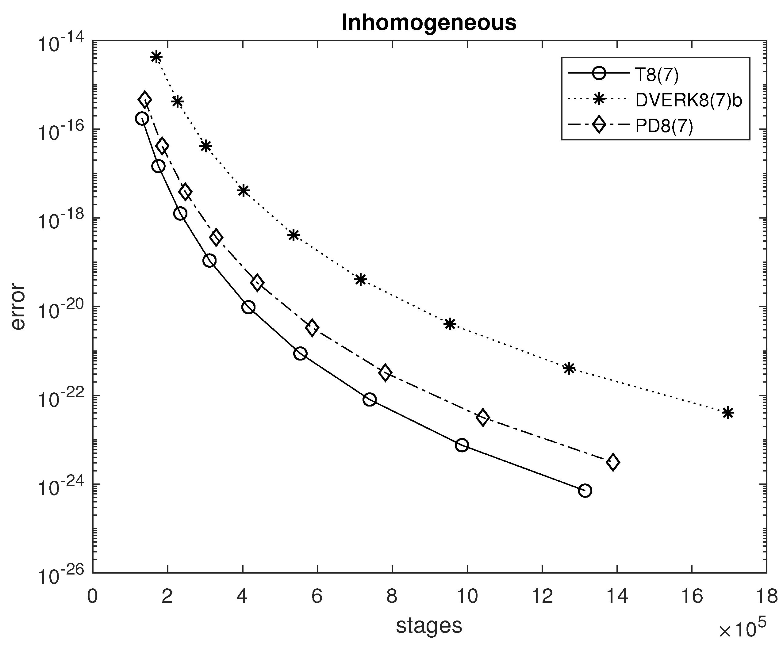
PD87 [12] and DVERK78 [17] are among the dominant pairs of their kind and are commonly used for higher accuracy computations. Their main advantage is the minimal truncation error coefficients norm $\parallel T^{\left(9\right)}{\parallel }_2$, i.e., the Euclidean norm of the 286 error coefficients of ninth order (see Table 1). A little later, Verner presented a more robust pair [18], which is implemented in Mathematica function NDSolve [19]. We name this pair DVERK78b and its coefficients can be retrieved (for use in quad-precision) easily by typing

In[2]:=NDSolve‘EmbeddedExplicitRungeKuttaCoefficients[8,34]

The minimization of the Euclidean norm $\parallel T^{\left(9\right)}{\parallel }_2$ is our main task here. Traditionally, we try also to keep the magnitude of the coefficients low when using double precision arithmetic (i.e., about 16 decimal digits). Then, a coefficient of size ${10}^5$ along with tolerance $\epsilon ={10}^{-11}$ would cause a severe test in the margins of available digits; however, in quadruple precision, we may admit these large coefficients even for tolerances as low as about ${10}^{-25}$. Thus, we may proceed in a new minimization process allowing the coefficients to grow.

In order to accomplish this we use the differential evolution (DE) technique [20]. DE is an iterative procedure; in every iteration, named generation g, we work with a “population” of individuals. i.e., here the free parameters form the decades

$$\left(c_2^{\left(g\right)},c_5^{\left(g\right)},c_6^{\left(g\right)},c_7^{\left(g\right)},\cdots {\widehat{w}}_{12}^{\left(g\right)},w_{13}^{\left(g\right)}\right),i=1,2,\cdots ,N,$$

with N the population size. An initial population

$$\left(c_2^{\left(0\right)},c_5^{\left(0\right)},c_6^{\left(0\right)},c_7^{\left(0\right)},\cdots {\widehat{w}}_{12}^{\left(0\right)},w_{13}^{\left(0\right)}\right),i=1,2,\cdots ,N,$$

is randomly created in the first step of the method. Thus, at first we form a fitness function that evaluates $\parallel T^{\left(9\right)}{\parallel }_2$. Following that, the fitness function is assessed for each member in the initial population. A three-phases sequential approach updates all of the persons participating in each iteration (generation) g. Differentiation, crossover, and selection are the phases involved. For the latter method, we utilized MATLAB [21] Software DeMat [22]. A MATLAB version of the algorithm is implemented for this purpose.

Among the various decades we obtained by the technique applied, we concluded the following coefficients that are given in Mathematica format to ensure that are error free. The following coefficients are ready for use with build-in function NDSolve.

In[2]:=T87evec=  {10839870895445/185203278486104297,0,0,0,0,70876466420204/75470597442438275,

            -16496614726651/75468957694148719,54859577937538923405/14355606386435513,

          17895137500075704819/2362101251104030,-969063659258770673/19161965088242370,

-39193463899416576680/3455993185375433,-973424986199410385/155592419305288032,16491/120125}/10;

T87cvec=       {3102/110773,41448895555141/353624691619188,41448895555141/235749794412792,

    49442/119883,51187/105369,61011/376738,77114/79499,147909751614626799/152923788158104127,

                                    74279/78046,72043/74409,1,1};

T87amat={                                        {3102/110773},

           {-17033458900934993/132978864382888258,17659313382611255/71989792689293837},

                 {41448895555141/942999177651168,0,41448895555141/314333059217056},

          {33544131897542527/99303639017753176,0,-123806032279621065/100880451772826828,

                                80881552191452041/62126727673226683},

           {3901178494518027/70202052982346435,0,0,12244602153330846/48744104078022083,

                                11363782051482252/63479278340035273},

           {7281184019796491/108906123149933189,0,0,8912953764743186/75237479424494327,

             -1193193435755019/24043824215671157,3001381510813201/114340525306552991},

       {-297808918551351805/103302384399153762,0,0,-2387409947307450796/38235137422988677,

   -320655295147743895/172685972706995386,266830735262229145/73369592821183637,8174527/126711},

        {-312230898179118543/111335375555652709,0,0,-5921685522031592717/97516557935639304,

            -122516042059134140/66440638491697461,143089054978597281/39930960285352934,

              1966780853930863533/31340008936176199,27204097600957/30119714219091834},

        {-497327926559154029/208366132906665209,0,0,-2070519061247416919/40105304012179956,

            -139926368413626755/79789745208684688,436822604663916242/133157501626893287,

             4951999978536596383/92678477827402881,-1662171172972759/32043786293542537,

                                   320510318790859/5467452906511140},

         {-267997292446794835/94625648159795289,0,0,-1326916430444389167/21635054137957163,

             -50510473210813287/27322222661367848,680595213260915461/188925642391189177,

              1090597603926315985/17207867085312708,-818226826952911/56758278493554744,

               794276136679319/44163223221855014,-495594365453263/165024671142376612},

         {-286074472550848766/70568381571246193,0,0,-2666282586603439301/29766446888618900,

             -394981932622811234/181671027945865139,354437914440687571/72293255173230666,

            1737172167669457231/18855481952627537,-1908527156826626453/17978177470082379,

            14359180611877865064/20075894067162869,-1863006586402493967/31715262582627044,

                                 -5146117877451253921/9346764321565133},

        {-2286460617615599450/148215689608432541,0,0,-21511651826330234931/52669819756106150,

             -949790098629780736/69310896259636617,2488552272190713800/64326656295428697,

            14577683994864478388/35463253730030943,-34626716477448076238/6579786536866391,

            267076469802229885930/7436961774107587,-15666088518007151408/5323429123670105,

                               -39614246945332388915/1429199330541022,0}};

T87bvec=       {959469921003535/20735873900418433,0,0,0,0,83661087663817387/226096222469839182,

              228743606234324881/883020026679163794,3544120671195926375/8063503515187523,

               164403934540876/64548125027903185,1872154679941434671/50440600905843744,

      -3908844507545666995/8324248434152054,-402658040159189839/58491143516062232,16491/120125};

T87Coefficients[8,p_]:=N[{T87amat,T87bvec,T87cvec,T87evec},p];

MATLAB furnished the free coefficients in double precision (see, e.g., $c_2,c_5$, etc., in vector T87cvec). Considering these free coefficients as exact, we were able to extract the rest coefficients in quadruple precision as listed above.

Another issue that is interesting when dealing with (1) is the existence of large stability intervals. For the eighth order formula (which the solution propagated) we form the polynomial

$$\begin{array}{ccc}\hfill I\left(t\right)& =& 1+t+\frac{1}{2}{t}^2+\frac{1}{3!}{t}^3+\frac{1}{4!}{t}^4+\frac{1}{5!}{t}^5+\frac{1}{6!}{t}^6+\frac{1}{7!}{t}^7+\frac{1}{8!}{t}^8\hfill \\ & & +(w·A^7·c)·t^9+(w·A^8·c)·t^{10}+(w·A^9·c)·t^{11}+(w·A^{10}·c)·t^{12}.\hfill \end{array}$$

There is no need to add the term $t^{13}$ since $a_{13,12}=0$ and in consequence $w·A^{11}·c=0$. The real stability interval has the form $(t_0,0)$ with $t_0<0$ and $\left|I\right(t\left)\right|\le 1$ holds for all $t>t_0$.

The basic characteristics of the methods presented here can be found in

Table 2. Basic characteristics of the RK pairs considered.

Pair	Maximum Coefficient	Real Stability Interval	${∥\mathit{T}{}^{\left(9\right)}∥}_2$
DVERK8(7)b	5.9	(−4.52, 0)	7.55 · 10−6
PD8(7)	16.7	(−5.16, 0)	4.51 · 10−6
T8(7)	43,463.3	(−5.08, 0)	3.89 · 10−8

. It is obvious that our objective was met by far with RK8(7).

4. Numerical Results

The Runge–Kutta pairs of orders eight and seven chosen for comparison are the following

• DVERK78b: The pair proposed by Verner [18].
• PD87: The pair of [12] with coefficients in an enhanced 34 decimal digits version.
• T87: The pair constructed here.

The above selection is justified by the chosen methods being the most used ones. DVERK78b is also implemented in MAPLE function dsolve [23] and its coefficients can be retrieved using MATHEMATICA (see In[1] above).

All the problems were run in MATHEMATICA using the NDSolve function and exploiting the capabilities offered for explicit Runge–Kutta pairs [24].

The problems of the tests are the following:

4.1. Inhomogeneous Equation

The first test problem chosen is the inh○m○gene○us equation:

$$\begin{array}{ccc}\hfill {\zeta }_1^{\prime }& =& {\zeta }_2\hfill \\ \hfill {\zeta }_2^{\prime }& =& -100{\zeta }_1\left(x\right)+99·sin\left(x\right),\hfill \end{array}$$

${\zeta }_1\left(0\right)=1,{\zeta }_2\left(0\right)=11,$ with analytical solution [25]

$${\zeta }_1\left(x\right)=cos\left(10x\right)+sin\left(10x\right)+sin\left(x\right),{\zeta }_2\left(x\right)={\zeta }_1^{\prime }\left(x\right).$$

We integrated this problem in the interval $x\in \left[0,20\pi \right]$ for tolerances $\epsilon ={10}^{-16},$${10}^{-17},\cdots ,{10}^{-23},{10}^{-24}$. We then recorded the cost (in function evaluations) versus the achieved end-point accuracy for the three pairs. The corresponding efficiency plots are shown in Figure 1. The rightmost lower circle in Figure 1 may produced in Mathematica after typing:

In[3]:=Needs["DifferentialEquations‘NDSolveProblems‘"];

In[4]:=Needs["DifferentialEquations‘NDSolveUtilities‘"];

In[5]:=system=NDSolveProblem[{{y1’[t]==y2[t],y2’[t]==-100*y1[t]+99*Sin[t]},

                 {y1[0]==1,y2[0]==11},{y1[t],y2[t]},{t,0,20*Pi},{},{},{}}];

In[6]:=CompareMethods[system, {1, 11}, {{"ExplicitRungeKutta",

                                        "Coefficients" -> T87Coefficients,

                        "DifferenceOrder" -> 8, "StiffnessTest" -> False}},

           WorkingPrecision -> 33, AccuracyGoal -> 24, PrecisionGoal -> 24]

Out[6]={{{101128,0},1314666,7.12428*10^-25}}

i.e., we spent about $13.1·{10}^5$ stages and achieved more than 24 digits of accuracy. Observe that the solution at the initial and at the end-point coincide.

4.2. Brusselator

Secondly we tried the Brusselator problem [26], which is formed after the laws of chemical kinetics. A simplified version is given in [27] (p. 116), and has the form

$$\begin{array}{ccc}\hfill {\zeta }_1^{\prime }& =& 1+{\zeta }_1^2{\zeta }_2-4{\zeta }_1\hfill \\ \hfill {\zeta }_2^{\prime }& =& 3{\zeta }_1-{\zeta }_1^2{\zeta }_2,\hfill \end{array}$$

${\zeta }_1\left(0\right)=1.5,{\zeta }_2\left(0\right)=3$. See also [28] (p. 22).

The analytical solution is not available. An end-point approximation of the solution was found by a very accurate integration. We then integrated this problem in the interval $x\in \left[0,20\right]$ for tolerances $\epsilon ={10}^{-16},{10}^{-17},$$\cdots ,{10}^{-23},{10}^{-24}$. We also recorded the cost (in function evaluations) versus the achieved end-point accuracy for the three pairs. The corresponding efficiency plots are shown in Figure 2.

4.3. Two Body Problem

We continued with the Kepler problem with eccentricity $0.5$ as in [29] which shares the following equations

$${\zeta }_1^{\prime }={\zeta }_3,{\zeta }_2^{\prime }={\zeta }_4,{\zeta }_3^{\prime }=-\frac{{\zeta }_1}{{\left(\sqrt{{\zeta }_1^2+{\zeta }_2^2}\right)}^3},{\zeta }_4^{\prime }=-\frac{{\zeta }_2}{{\left(\sqrt{{\zeta }_1^2+{\zeta }_2^2}\right)}^3}$$

with initial conditions ${\zeta }_1\left(0\right)=0.5,{\zeta }_2\left(0\right)=0,{\zeta }_3\left(0\right)=0,{\zeta }_4\left(0\right)=\sqrt{3}.$

The analytical solution is shown in [30]. We also integrated this problem in the interval $x\in \left[0,6\pi \right]$ for tolerances $\epsilon ={10}^{-16},{10}^{-17},$$\cdots ,{10}^{-23},{10}^{-24}$. We then recorded the cost versus the achieved end-point accuracy for the three pairs. The corresponding efficiency plots are shown in Figure 3.

4.4. The Euler Problem

We finally tried the Euler problem as given in [27] (p. 244). Namely

$$\begin{array}{ccc}\hfill {\zeta }_1^{\prime }& =& -2{\zeta }_2{\zeta }_3\hfill \\ \hfill {\zeta }_2^{\prime }& =& \frac{5}{4}{\zeta }_1{\zeta }_3\hfill \\ \hfill {\zeta }_3^{\prime }& =& -\frac{1}{2}{\zeta }_1{\zeta }_2+g\left(x\right)\hfill \end{array}$$

and the exterior force given as

$$g\left(x\right)=\{\begin{array}{cc}\frac{1}{4}{sin}^{2}x& \mathrm{when}4\pi \ge x\ge 3\pi \hfill \\ 0& \mathrm{otherwise}\hfill \end{array}$$

with initial values ${\zeta }_1\left(0\right)=1,{\zeta }_2\left(0\right)=0,{\zeta }_3=0.9.$

The analytical solution is not available. An end-point approximation of the solution was found by a very accurate integration. We then integrated this problem in the interval $x\in \left[0,20\right]$ for tolerances $\epsilon ={10}^{-16},{10}^{-17},$$\cdots ,{10}^{-23},{10}^{-24}$. We also recorded the cost versus the achieved end-point accuracy for all three pairs. The corresponding efficiency plots are shown in Figure 4.

Interpreting the results we observe a clear and wide distance in favor of our new proposal since it takes advantage of the significantly smaller truncation error.

5. Conclusions

A new Runge–Kutta pair of orders eight and seven is proposed for use in high precision computations. A smaller truncation error is achieved at an affordable cost of larger magnitude of the coefficients. Its performance is illustrated in a set of relevant problems.

References

1. Butcher, J.C. Implicit Runge-Kutta processes. Math. Comput. 1964, 18, 50–64. [Google Scholar] [CrossRef]
2. Butcher, J.C. On Runge-Kutta processes of high order. J. Austral. Math. Soc. 1964, 4, 179–194. [Google Scholar] [CrossRef]
3. Tsitouras, C.; Papakostas, S.N. Cheap error estimation for Runge-Kutta methods. SIAM J. Sci. Comput. 1999, 20, 2067–2088. [Google Scholar] [CrossRef]
4. Cassity, C.R. The complete solution of the fifth order Runge-Kutta equations. SIAM J. Numer. Anal. 1969, 6, 432–436. [Google Scholar] [CrossRef]
5. Butcher, J.C. The Numerical Analysis of ODEs: Runge-Kutta and General Linear Methods; Wiley: Chichester, UK, 1987. [Google Scholar]
6. Fehlberg, E. Classical Fifth, Sixth, Seventh, and Eighth Order Runge-Kutta Formulas with Stepsize Control, TRR-287; NASA: Marshall Space Flight Center: Huntsville, AL, USA, 1968. [Google Scholar]
7. Famelis, I.T.; Papakostas, S.N.; Tsitouras, C. Symbolic derivation of Runge-Kutta order conditions. J. Symbolic Comput. 2004, 37, 311–327. [Google Scholar] [CrossRef]
8. Oliver, J. A Curiosity of Low-Order Explicit Runge-Kutta Methods. Math. Comput. 1975, 29, 1032–1036. [Google Scholar] [CrossRef]
9. Tsitouras, C. Explicit Runge-Kutta methods for starting integration of Lane–Emden problem. Appl. Math. Comput. 2019, 354, 353–364. [Google Scholar] [CrossRef]
10. Papakostas, S.N.; Tsitouras, C.; Papageorgiou, G. A general family of explicit Runge-Kutta pairs of orders 6(5). SIAM J. Numer. Anal. 1996, 33, 917–936. [Google Scholar] [CrossRef]
11. Verner, J.H. Explicit Runge-Kutta methods with estimates of the local truncation error. SIAM J. Numer. Anal. 1978, 15, 772–790. [Google Scholar] [CrossRef]
12. Prince, P.J.; Dormand, J.R. High order embedded Runge-Kutta formulae. J. Comput. Appl. Math. 1981, 7, 67–75. [Google Scholar] [CrossRef] [Green Version]
13. Papakostas, S.N. Algebraic Analysis and Development of Numerical ODE Solvers of the Runge-Kutta Type. Ph.D. Thesis, National Technical University, Athens, Greece, 1996. Available online: https://www.didaktorika.gr/eadd/handle/10442/6561 (accessed on 8 August 2022).
14. Papakostas, S.N.; Tsitouras, C. High Phase-Lag-order Runge-Kutta and Nyström pairs. SIAM J. Sci. Comput. 1999, 21, 747–763. [Google Scholar] [CrossRef]
15. Verner, J.H. A contrast of some Runge-Kutta formula pairs. SIAM J. Numer. Anal. 1990, 27, 1332–1344. [Google Scholar] [CrossRef]
16. Verner, J.H. Some Runge-Kutta formula pairs. SIAM J. Numer. Anal. 1991, 28, 496–511. [Google Scholar] [CrossRef]
17. Verner, J.H. Numerically optimal Runge–Kutta pairs with interpolants. Numer. Algor. 2010, 53, 383–396. [Google Scholar] [CrossRef]
18. Verner, J.H. Available online: https://www.sfu.ca/~jverner/RKV87.IIa.Robust.00000754677.081208.FLOAT40OnWeb (accessed on 8 August 2022).
19. NDSolve: Mathematica Function. Available online: https://reference.wolfram.com/language/ref/NDSolve.html?q=NDSolve (accessed on 8 August 2022).
20. Storn, R.; Price, K. Differential evolution—A simple and efficient heuristic for global optimization over continuous spaces. J. Glob. Optim. 1997, 11, 341–359. [Google Scholar] [CrossRef]
21. MATLAB Version R2019b; The Mathworks, Inc.: Natick, MA, USA, 2019.
22. Storn, R.; Price, K.; Neumaier, A.; Zandt, J.V. DeMat. Available online: https://github.com/mikeagn/DeMatDEnrand (accessed on 25 March 2022).
23. dsolve, Maple Function. Available online: https://www.maplesoft.com/support/help/maple/view.aspx?path=dsolve/dverk78 (accessed on 8 August 2022).
24. “ExplicitRungeKutta” for NDSolve. Available online: https://reference.wolfram.com/language/tutorial/NDSolveExplicitRungeKutta.html (accessed on 8 August 2022).
25. Tsitouras, C.; Simos, T.E. High algebraic, high phase-lag order embedded Numerov-type methods for oscillatory problems. Appl. Math. Comput. 2002, 131, 201–211. [Google Scholar] [CrossRef]
26. Lefever, R.; Nicolis, G. Chemical Instabilities and sustained oscillations. J. Theor. Biol. 1971, 30, 267–284. [Google Scholar] [CrossRef]
27. Hairer, E.; Nørsett, S.P.; Wanner, G. Solving Ordinary Differential Equations I: Nonstiff Problems; Springer: Berlin, Germany, 1993. [Google Scholar]
28. Sofroniou, M.; Knapp, R. Advanced numerical differential equation solving in Mathematica. In Wolfram Mathematica Tutorial Collection; Wolfram Research: Champaign, IL, USA, 2008. [Google Scholar]
29. Tsitouras, C. A tenth order symplectic Runge-Kutta and Nyström method. Cele. Mech. Dynam. Astron. 1999, 74, 223–230. [Google Scholar] [CrossRef]
30. Tsitouras, C.; Papageorgiou, G. Runge-Kutta Interpolants Based on Values from Two Successive Integration Steps. Computing 1990, 43, 255–266. [Google Scholar] [CrossRef]
Figure 1. Efficiency plots for the inhomogeneous equation.
Mathematics 10 03247 g001
Figure 2. Efficiency plots for the Brusselator.
Mathematics 10 03247 g002
Figure 3. Efficiency plots for the Kepler problem.
Mathematics 10 03247 g003
Figure 4. Efficiency plots for the Euler problem.
Mathematics 10 03247 g004