Lie Symmetry Classification and Qualitative Analysis for the Fourth-Order Schrödinger Equation

Abstract

The Lie symmetry analysis for the study of a $1+n$ fourth-order Schrödinger equation inspired by the modification of the deformation algebra in the presence of a minimum length is applied. Specifically, we perform a detailed classification for the scalar field potential function where non-trivial Lie symmetries exist and simplify the Schrödinger equation. Then, a qualitative analysis allows for the reduced ordinary differential equation to be analysed to understand the asymptotic dynamics.

1. Introduction

The Lie symmetry analysis is a systematic approach to the study of nonlinear differential equations [1,2]. The existence of a symmetry vector for a given differential equation indicates the existence of invariant functions, which are then used to simplify the differential equation and, when it is possible, determine exact or analytic solutions [3,4,5,6,7,8,9,10,11,12,13]. Moreover, symmetries can be used for the determination of conservation laws and also identify equivalent dynamical systems [14,15,16,17]. Finally, the Lie symmetry analysis covers a wide range of applications in all areas of applied mathematics. In this work, we are interested in the symmetry classification of a higher-order differential equation.

Consider the fourth-order partial differential equations, known as the Schrödinger equation

$$i\frac{\partial \mathrm{\Psi }}{\partial t}+\alpha \Delta \mathrm{\Psi }+\gamma {\Delta }^2\mathrm{\Psi }+V\left(\mathrm{\Psi }\right)=0,$$

(1)

with $\gamma \ne 0$, $\Delta$ the Laplace operator $\Delta =\frac{1}{\sqrt{\left|g\right|}}\frac{\partial }{\partial x^{\mu }}\left(\sqrt{\left|g\right|}{g}^{\mu \nu }\right)\frac{\partial }{\partial x^{\nu }}$, $g_{\mu \nu }$ is the metric tensor, which describes the physical space. The fourth-order Schrödinger equation was introduced in [18,19] in order to investigate the effects of the presence of small fourth-order dispersion terms in the propagation of laser beams in a bulk medium with Kerr nonlinearity. For $V\left(\mathrm{\Psi }\right)={\left|\mathrm{\Psi }\right|}^{2p}\mathrm{\Psi }$, the stability of solitons was investigated by Karpman in [18]. It was found that when $g_{\mu \nu }$ is the Euclidian manifold, then for $pdim\left(g\right)<4$, the soliton solutions are stable. Since then, the fourth-order Schrödinger equation has been the subject of study in various articles in the literature (see, for instance, [20,21,22,23,24,25,26,27]). Indeed, the soliton instabilities of the equation for $V\left(\mathrm{\Psi }\right)={\left|\mathrm{\Psi }\right|}^{2p}\mathrm{\Psi }$ are related to nonlinear fibre optics and optical solutions in gyrotropic media [28]. Moreover, optical and other soliton solitons have been constructed with the use of Equation (1) to describe localised electromagnetic waves that spread in nonlinear dispersive media [29]. In [29], the Ricatti–Bernoulli sub-ODE method and the modified Tanh-Coth method are applied for the derivation of solitons for Equation (1) and $V\left(\mathrm{\Psi }\right)=V_0\left({\left|\mathrm{\Psi }\right|}^{2p}+\epsilon {\left|\mathrm{\Psi }\right|}^{4p}\right)\mathrm{\Psi }$. For more physical applications and the relation of the free parameters $\alpha ,\gamma$ and p to physical phenomena, see reference [29]. Equation (1) has also been used for the description of bright and grey/dark soliton-like solutions in the context of Madelung’s fluid [30]. The orbital stability of standing wave solution in the context of Hamiltonian systems was investigated in [31] by constructing a Lyapunov function. Finally, the Cauchy problem for an inhomogeneous equation constructed by (1) was studied in [32].

Last but not least, we recall that for $\gamma \to 0$, the usual Schrödinger equation of quantum mechanics is recovered.

However, Equation (1) also describes the modified Schrödinger equation for a particle in the context of the Generalised Uncertainty Principle (GUP). Indeed, GUP can be used for the construction and derivation of Equation (1).

GUP has its origin in the existence of a minimal length of the order of the Planck length ($l_{PL}$). The latter is a standard prediction of different quantum physics and gravity approaches, that is, from string theory, noncommutative geometry, and others [33,34,35,36]. Specifically, the minimal length in Heisenberg’s Uncertainty Principle [37] is introduced. For a review on GUP, we refer the reader to [38].

In the simplest case of quadratic GUP, the modified Heisenberg’s Uncertainty Principle reads

$$\Delta X_{\mu }\Delta P_{\nu }⩾\frac{\hslash }{2}[{\delta }_{ij}(1+\beta P^2)+2\beta P_{\mu }{P}_{\nu }].$$

(2)

Consequently, the deformed algebra follows [39,40],

$$[X_{\mu },P_{\nu }]=i\hslash [{\delta }_{ij}(1-\beta P^2)-2\beta P_{\mu }{P}_{\nu }],$$

(3)

where $\beta$ is the parameter of deformation defined by $\beta ={\beta }_0/{M_{Pl}^2{c}^2=\beta }_0{\ell }_{Pl}^2/2{\hslash }^2$, where $M_{Pl}$ is the Planck mass, ${\ell }_{Pl}$ ($\approx {10}^{-35}m)$ is the Planck length and $M_{Pl}{c}^2$ (≈$1.2\times {10}^{19}$ GeV) the Planck energy, such that ${\beta }^2\to 0$. Thus, we can consider the coordinate representation of the modified momentum operator $P_{\mu }=p_{\mu }(1-\beta p^2)$[40], while keeping $X_{\mu }=x_{\mu }$ undeformed. Thus, the time-independent Schrödinger equation reads

$$\left(g^{\mu \nu }{P}_{\mu }{P}_{\nu }-{\left(mc\right)}^2\right)\mathrm{\Psi }=0.$$

(4)

That is,

$$-2\beta {\hslash }^2{\Delta }^2\mathrm{\Psi }+\Delta \mathrm{\Psi }+{\left(\frac{mc}{\hslash }\right)}^2\mathrm{\Psi }=0,$$

(5)

assuming terms with ${\beta }^2\to 0$. The fourth-order Equation (5) is the static version of (1) for $V\left(\mathrm{\Psi }\right)$, which is a linear function. For some recent applications of GUP in physical theories, see [41,42,43,44,45] and references therein.

In the following, we perform a complete classification of function $V\left(\mathrm{\Psi }\right)$ according to the admitted Lie point symmetries of Equation (1). Such a classification scheme was proposed in the previous century by Ovsiannikov, where the Lie point symmetries for the nonlinear equation $u_t={\left(f\left(u\right)u_x\right)}_x$ were classified [46], leading to new interesting problems in applied mathematics and physics [47,48,49,50,51,52]. Apart from the analysis of symmetries, the concept of asymptotic solutions and boundary layers is essential in this context [53].

The plan of the paper is as follows. In Section 2, we present the basic properties and definitions for the theory of Lie symmetries of differential equations, and we introduce the concept of the boundary layer. In Section 3, we present our classification scheme for the Lie point symmetries of the fourth-order Schrödinger equation. We present some applications of the Lie point symmetries for the construction of similarity solutions in Section 4. Finally, in Section 5, we summarise our results.

2. Preliminaries

A differential equation may be considered as a function $H=H(x^i,u^A,u_{,i}^A,u_{,ij}^A,\cdots )$ in the space $B=B(x^i,u^A,u_{,i}^A,u_{,ij}^A,\cdots )$, where $x^i$ are the independent variables, and $u^A$ are the dependent variables. In our consideration for Equation (1) $x^i=\left(t,x^{\mu }\right)$ and $u^A\left(x^i\right)=\mathrm{\Phi }\left(x^i\right).$

2.1. Lie Symmetry Vector

Consider now the infinitesimal transformation

$$\begin{array}{cc}\hfill {\overline{x}}^i& =x^i+\epsilon {\xi }^i(x^k,u^B),\hfill \end{array}$$

(6)

$$\begin{array}{cc}\hfill {\overline{u}}^A& ={\overline{u}}^A+\epsilon {\eta }^A(x^k,u^B),\hfill \end{array}$$

(7)

with the generator of the vector field

$$\mathbf{X}={\xi }^i(x^k,u^B){\partial }_{x^i}+{\eta }^A(x^k,u^B){\partial }_{u^A}.$$

(8)

The generator $\mathbf{X}$ of the infinitesimal transformation (6), () is a Lie point symmetry for the function H if there exists a function $\lambda$ such that the following condition holds [1,2]

$${\mathbf{X}}^{\left[N\right]}\left(H\right)=\lambda H,modH=0,$$

(9)

where

$${\mathbf{X}}^{\left[N\right]}=\mathbf{X}+{\eta }_{\left[i\right]}^A{\partial }_{u_i^A}+{\eta }_{\left[ij\right]}^A{\partial }_{u_{ij}^A}+\cdots +{\eta }_{\left[ij\cdots j_N\right]}^A{\partial }_{u_{ij\cdots j_N}^A}$$

(10)

is the $n^{th}$ prolongation vector

$${\eta }_{\left[i\right]}^A={\eta }_{,i}^A+u_{,i}^B{\eta }_{,B}^A-{\xi }_{,i}^j{u}_{,j}^A-u_{,i}^A{u}_{,j}^B{\xi }_{,B}^j$$

(11)

with

$$\begin{array}{cc}\hfill {\eta }_{\left[ij\right]}^A& ={\eta }_{,ij}^A+2{\eta }_{,B(i}^A{u}_{,j)}^B-{\xi }_{,ij}^k{u}_{,k}^A+{\eta }_{,BC}^A{u}_{,i}^B{u}_{,j}^C-2{\xi }_{,\left(i\right|B|}^k{u}_{j)}^B{u}_{,k}^A\hfill \\ \hfill & -{\xi }_{,BC}^k{u}_{,i}^B{u}_{,j}^C{u}_{,k}^A+{\eta }_{,B}^A{u}_{,ij}^B-2{\xi }_{,(j}^k{u}_{,i)k}^A-{\xi }_{,B}^k\left(u_{,k}^A{u}_{,ij}^B+2u_{(,j}^B{u}_{,i)k}^A\right),\hfill \end{array}$$

(12)

and in general

$${\eta }_{\left[ij\cdots j_N\right]}^A=D_{j_n}\left({\eta }_{ij\cdots j_{n-1}}^A\right)-u_{ij\cdots k}^A{D}_{j_N}{\xi }^k.$$

(13)

The existence of a Lie point symmetry in a given differential equation is essential for simplifying the differential equation through the similarity transformations. Indeed, from a specific Lie symmetry vector, one may define the following Lagrange system

$$\frac{d{x}^i}{{\xi }^i}=\frac{d{u}^A}{{\eta }^A}=\frac{d{u}_i^A}{{\eta }_{\left[i\right]}^A}=\frac{d{u}_{ij}^A}{{\eta }_{\left[ij\right]}^A}=\cdots$$

(14)

whose solution provides the characteristic functions $W^{\left[0\right]}\left(x^k,u^A\right)$, $W^{\left[1\right]}\left(x^k,u^A,u_i^A\right)$, etc. These functions can be used to define the corresponding similarity transformation.

2.2. The Concept of a Boundary Layer

In the following, we briefly discuss the concept of boundary layers to investigate the asymptotic behaviour of nonlinear differential equations, following the notation presented in [53].

Assume the function ${\psi }_{\epsilon }\left(\tau \right)$ is defined on a domain $D\subset {\mathbb{R}}^n$ where $\epsilon$ is a small parameter. Consider now that there exists a connected subset $S\subset D$ with dimensions less or equal to n, such that ${\psi }_{\epsilon }\left(\tau \right)$ has no regular expansion in each subset $E\subset D$ with $E\cap S\ne \varnothing$. Then, a neighbourhood of S in D, with a size to be determined, is a boundary layer of the function ${\psi }_{\epsilon }\left(\tau \right)$[53]. Suppose $n=1$ and let ${\tau }_0\in S$, and suppose that near ${\tau }_0$ the boundary layer is characterised in size by the order function $\delta \left(\epsilon \right)$. For the analysis of the behaviour of ${\psi }_{\epsilon }$ near the boundary layer, we consider the map ${\psi }_{\epsilon }\left(\tau \right)={\psi }_{\epsilon }({\tau }_0+\delta \left(\epsilon \right)\xi )={\varphi }_{\epsilon }^{\ast }\left(\xi \right)$, where $\xi =\frac{\tau -{\tau }_0}{\delta \left(\epsilon \right)}$. When $\delta \left(\epsilon \right)=O\left(1\right)$, parameter $\xi$ is called a local variable. Hence, the concept is based on the construction of the approximation of function ${\varphi }_{\epsilon }^{\ast }\left(\xi \right)$ as ${\varphi }_{\epsilon }^{\ast }\left(\xi \right)={\sum }_n{\delta }_n^{\ast }\left(\epsilon \right){\psi }_n\left(\xi \right)$ with ${\delta }_n^{\ast }\left(\epsilon \right)$, $n=0,1,2,\cdots$ an asymptotic sequence.

For more details on the method and various applications, we refer the reader to [53].

3. Symmetry Classification for the Fourth-Order Schrödinger Equation

Before we proceed with the symmetry classification, we set without loss of generality $\gamma =1$, and by a change in transformation on the variable t, we can remove the coefficient i. Hence, Equation (1) can be written in the equivalent form

$$\frac{\partial \mathrm{\Psi }}{\partial t}+\alpha \Delta \mathrm{\Psi }+{\Delta }^2\mathrm{\Psi }+V\left(\mathrm{\Psi }\right)=0.$$

(15)

Moreover, with the use of the new variable $\mathrm{\Phi }=\Delta \mathrm{\Psi }$, the fourth-order differential Equation (15) is written as the following Schrödinger–Poisson system

$$\begin{array}{ccc}\hfill \frac{\partial \mathrm{\Psi }}{\partial t}+\Delta \mathrm{\Phi }+\alpha \mathrm{\Phi }+V\left(\mathrm{\Psi }\right)& =& 0,\hfill \end{array}$$

(16)

$$\begin{array}{ccc}\hfill \mathrm{\Phi }-\Delta \mathrm{\Psi }& =& 0.\hfill \end{array}$$

(17)

Assume now the generic vector field

$$X={\xi }^t\left(t,x^{\mu }.\mathrm{\Psi },\mathrm{\Phi }\right){\partial }_t+{\xi }^{\mu }\left(t,x^{\mu },\mathrm{\Psi },\mathrm{\Phi }\right){\partial }_{\mu }+{\eta }^{\mathrm{\Psi }}\left(t,x^{\mu },\mathrm{\Psi },\mathrm{\Phi }\right){\partial }_{\mathrm{\Psi }}+{\eta }^{\mathrm{\Phi }}\left(t,x^{\mu },\mathrm{\Psi },\mathrm{\Phi }\right){\partial }_{\mathrm{\Phi }},$$

(18)

where in order to be the generator of a one-parameter point transformation in the space of variables $\left\{x^{\mu },\mathrm{\Psi }\right\},$ it should be ${\xi }_{,\mathrm{\Phi }}^t=0$, ${\xi }_{,\mathrm{\Phi }}^{\mu }=0$ and ${\eta }_{,\mathrm{\Phi }}^{\mathrm{\Psi }}=0$.

The 2^ndprolongation vector reads

$$X^{\left[2\right]}=X+{\eta }_{\left[t\right]}^{\mathrm{\Psi }}{\partial }_{{\mathrm{\Psi }}_t}+{\eta }_{\left[\mu \right]}^{\mathrm{\Psi }}{\partial }_{{\mathrm{\Psi }}_{\mu }}+{\eta }_{\left[t\right]}^{\mathrm{\Phi }}{\partial }_{{\mathrm{\Phi }}_t}+{\eta }_{\left[\mu \right]}^{\mathrm{\Phi }}{\partial }_{{\mathrm{\Phi }}_{\mu }}+{\eta }_{\left[\mu \nu \right]}^{\mathrm{\Psi }}{\partial }_{{\mathrm{\Psi }}_{\mu \nu }}+{\eta }_{\left[\mu \nu \right]}^{\mathrm{\Phi }}{\partial }_{{\mathrm{\Phi }}_{\mu \nu }}.$$

(19)

Consequently, we apply the symmetry condition (9), and by using the geometric approach described in [54], we summarise the classification scheme in the following theorem.

Theorem 1.

The generic Lie point symmetry vector for the Schrödinger–Poisson system (16), (17) in an arbitrary background space $g_{\mu \nu }$, and for arbitrary function $V\left(\mathrm{\Psi }\right)$ is

$$X_G=a_1{\partial }_t+a_{\sigma }\mathbf{K}\left(x^{\kappa }\right){\partial }_{\mu },$$

(20)

where $\mathbf{K}\left(x^{\mu }\right)$ is an isometry for the metric tensor $g_{\mu \nu }$, that is $\left[\mathbf{K}\left(x^{\kappa }\right),g_{\mu \nu }\left(x^{\kappa }\right)\right]=0$.

However, for specific functional forms of the potential $V\left(\mathrm{\Psi }\right)$, the classification scheme is described as follows.

Theorem 2.

Let the metric tensor $g_{\mu \nu }\left(x^{\kappa }\right)$ and $\mathbf{K}\left(x^{\kappa }\right)$ describe the isometries of $g_{\mu \nu }\left(x^{\kappa }\right)$, and $\mathbf{H}\left(x^{\kappa }\right)$ is a proper Homothetic vector of $g_{\mu \nu }\left(x^{\kappa }\right)$, i.e., $\left[\mathbf{H}\left(x^{\kappa }\right),g_{\mu \nu }\left(x^{\kappa }\right)\right]=2g_{\mu \nu }\left(x^{\kappa }\right)$. Then, for special functional forms of $V\left(\mathrm{\Psi }\right)$, the generic symmetry vector for the Schrödinger–Poisson system (16), (17) is:

For $\alpha \ne 0$,

I: For $V\left(\mathrm{\Psi }\right)=V_0\mathrm{\Psi }$, the symmetry vector is $X_G^I=a_1{\partial }_t+a_{\sigma }\mathbf{K}\left(x^{\kappa }\right){\partial }_{\mu }+a_2\left(\mathrm{\Psi }{\partial }_{\mathrm{\Psi }}+\mathrm{\Phi }{\partial }_{\mathrm{\Phi }}\right)+a_3\left(F\left(t,x^{\kappa }\right){\partial }_U+F_{,\mu \nu }\left(t,x^{\kappa }\right){\partial }_{\mathrm{\Phi }}\right)$, where $F\left(t,x^{\kappa }\right)$ is a solution of the original system. The new coefficients in the vector field indicate the linearisation of the system.

For $\alpha =0$,

II: For $V\left(\mathrm{\Psi }\right)=0$, the generic symmetry vector is $X_G^{II}=a_1{\partial }_t+a_{\sigma }\mathbf{K}\left(x^{\kappa }\right){\partial }_{\mu }+a_2\left(\mathrm{\Psi }{\partial }_{\mathrm{\Psi }}+\mathrm{\Phi }{\partial }_{\mathrm{\Phi }}\right)+a_3\left(F\left(t,x^{\kappa }\right){\partial }_U+F_{,\mu \nu }\left(t,x^{\kappa }\right){\partial }_{\mathrm{\Phi }}\right)+a_4\left(4t{\partial }_t+\mathbf{H}\left(x^{\kappa }\right){\partial }_{\mu }-2\mathrm{\Phi }{\partial }_{\mathrm{\Phi }}\right)$.

III: For $V\left(\mathrm{\Psi }\right)=V_0\mathrm{\Psi }$, the generic symmetry vector is $X_G^{III}=a_1{\partial }_t+a_{\sigma }\mathbf{K}\left(x^{\kappa }\right){\partial }_{\mu }+a_2\left(\mathrm{\Psi }{\partial }_{\mathrm{\Psi }}+\mathrm{\Phi }{\partial }_{\mathrm{\Phi }}\right)+a_3\left(F\left(t,x^{\kappa }\right){\partial }_U+F_{,\mu \nu }\left(t,x^{\kappa }\right){\partial }_{\mathrm{\Phi }}\right)+a_4\left(4t{\partial }_t+\mathbf{H}\left(x^{\kappa }\right){\partial }_{\mu }-2\mathrm{\Phi }{\partial }_{\mathrm{\Phi }}-4V_{0}t\left(\mathrm{\Psi }{\partial }_{\mathrm{\Psi }}+\mathrm{\Phi }{\partial }_{\mathrm{\Phi }}\right)\right)$.

IV: For $V\left(\mathrm{\Psi }\right)=V_0{\mathrm{\Psi }}^{P+1},P\ne -1,0$, the generic symmetry vector is $X_G^{IV}=a_1{\partial }_t+a_{\sigma }\mathbf{K}\left(x^{\kappa }\right){\partial }_{\mu }+a_4\left(4t{\partial }_t+\mathbf{H}\left(x^{\kappa }\right){\partial }_{\mu }-2\mathrm{\Phi }{\partial }_{\mathrm{\Phi }}-\frac{4}{P}\left(\mathrm{\Psi }{\partial }_{\mathrm{\Psi }}+\mathrm{\Phi }{\partial }_{\mathrm{\Phi }}\right)\right)$.

V: For $V\left(\mathrm{\Psi }\right)=V_{0}exp\left(P\mathrm{\Psi }\right),P\ne 0$, the generic symmetry vector is $X_G^{IV}=a_1{\partial }_t+a_{\sigma }\mathbf{K}\left(x^{\kappa }\right){\partial }_{\mu }+a_4\left(4t{\partial }_t+\mathbf{H}\left(x^{\kappa }\right){\partial }_{\mu }-2\mathrm{\Phi }{\partial }_{\mathrm{\Phi }}-\frac{4}{P}\left({\partial }_{\mathrm{\Psi }}\right)\right)$.

It is easy to observe that the collineations of the underlying geometry generate the symmetries for the dynamical system of our study. Indeed, the isometries and the homothetic vectors construct the Lie symmetries. If a background geometry has no isometries and homothetic vector, then the admitted Lie symmetries for the dynamical system are the trivial symmetries. That connection of the Lie symmetries with the elements of the background geometry has been observed before for various differential equations [55,56]. Indeed, for the second-order Schrödinger equation, the Lie symmetries are constructed by the elements of the homothetic algebra of the geometry [56]. Thus, a similar physical interpretation can be given. The Lie symmetries generated by the isometries are related to the construction of differential operators generated by the conservation law of momentum for the classical particle. In contrast, the Lie symmetry constructed by the homothetic vector field is related to the derivation of scaling solutions. For more details, we refer the reader to [56].

We proceed with our analysis by considering specific metric tensor $g_{\mu \nu }$.

4. Application

Consider now that the metric tensor $g_{\mu \nu }$ is maximally symmetric and admit a homothetic vector field. Hence, $g_{\mu \nu }$ is necessary for the flat space. For simplicity of our calculations, assume further that $dim{g}_{\mu \nu }=1$. The one-dimensional flat space with line element $d{s}^2=d{x}^2$ admits the isometry ${\partial }_x$ and the proper Homothetic field $x{\partial }_x$.

Therefore the Schrödinger–Poisson system reads

$$\begin{array}{ccc}\hfill \frac{\partial \mathrm{\Psi }}{\partial t}+\frac{{\partial }^2\mathrm{\Phi }}{\partial x^2}+\alpha \mathrm{\Phi }+V\left(\mathrm{\Psi }\right)& =& 0,\hfill \end{array}$$

(21)

$$\begin{array}{ccc}\hfill \mathrm{\Phi }-\frac{{\partial }^2\mathrm{\Psi }}{\partial x^2}& =& 0.\hfill \end{array}$$

(22)

In the case where $\alpha \ne 0$, the generic vector field is $X^I=a_1{\partial }_t+a_2{\partial }_x$, for arbitrary potential function $V\left(\mathrm{\Psi }\right)$. From the elements of $X^I$, we can reduce the dynamical system into the static and the stationary cases. However, from the vector field ${\partial }_t+c{\partial }_x$ we reduce the dynamical system as follows

$$\begin{array}{ccc}\hfill -c\frac{\partial \mathrm{\Psi }}{\partial \xi }+\frac{{\partial }^2\mathrm{\Phi }}{\partial {\xi }^2}+\alpha \mathrm{\Phi }+V\left(\mathrm{\Psi }\right)& =& 0,\hfill \end{array}$$

(23)

$$\begin{array}{ccc}\hfill \mathrm{\Phi }-\frac{{\partial }^2\mathrm{\Psi }}{\partial {\xi }^2}& =& 0,\hfill \end{array}$$

(24)

where $\xi =x-ct$ is the new independent variable, and c describes the speed of the travelling wave. For a linear function $V\left(\mathrm{\Psi }\right),$ the closed-form solution of the system (23), (24) can be expressed in terms of exponential functions.

However, for $V\left(\mathrm{\Psi }\right)=V_0\mathrm{\Psi }$, there exist the additional possible reduction ${\partial }_t+c{\partial }_x+\beta \left(\mathrm{\Psi }{\partial }_{\mathrm{\Psi }}+\mathrm{\Phi }{\partial }_{\mathrm{\Phi }}\right)$, which provides the similarity transformation $\mathrm{\Psi }=e^{\beta t}\psi \left(\xi \right)$, $\mathrm{\Phi }=e^{\beta t}\varphi \left(\xi \right)$, $\xi =x-ct$ with a reduced system

$$\begin{array}{ccc}\hfill -c\frac{\partial \psi }{\partial \xi }+\frac{{\partial }^2\varphi }{\partial {\xi }^2}+\alpha \varphi +\beta \psi +V_0\psi & =& 0,\hfill \end{array}$$

(25)

$$\begin{array}{ccc}\hfill \varphi -\frac{{\partial }^2\psi }{\partial {\xi }^2}& =& 0.\hfill \end{array}$$

(26)

Let us focus now on the case where $\alpha =0$ and assume $V\left(\mathrm{\Psi }\right)=V_0{\mathrm{\Psi }}^{P+1}$ and $V\left(\mathrm{\Psi }\right)=V_{0}exp\left(P\mathrm{\Psi }\right)$.

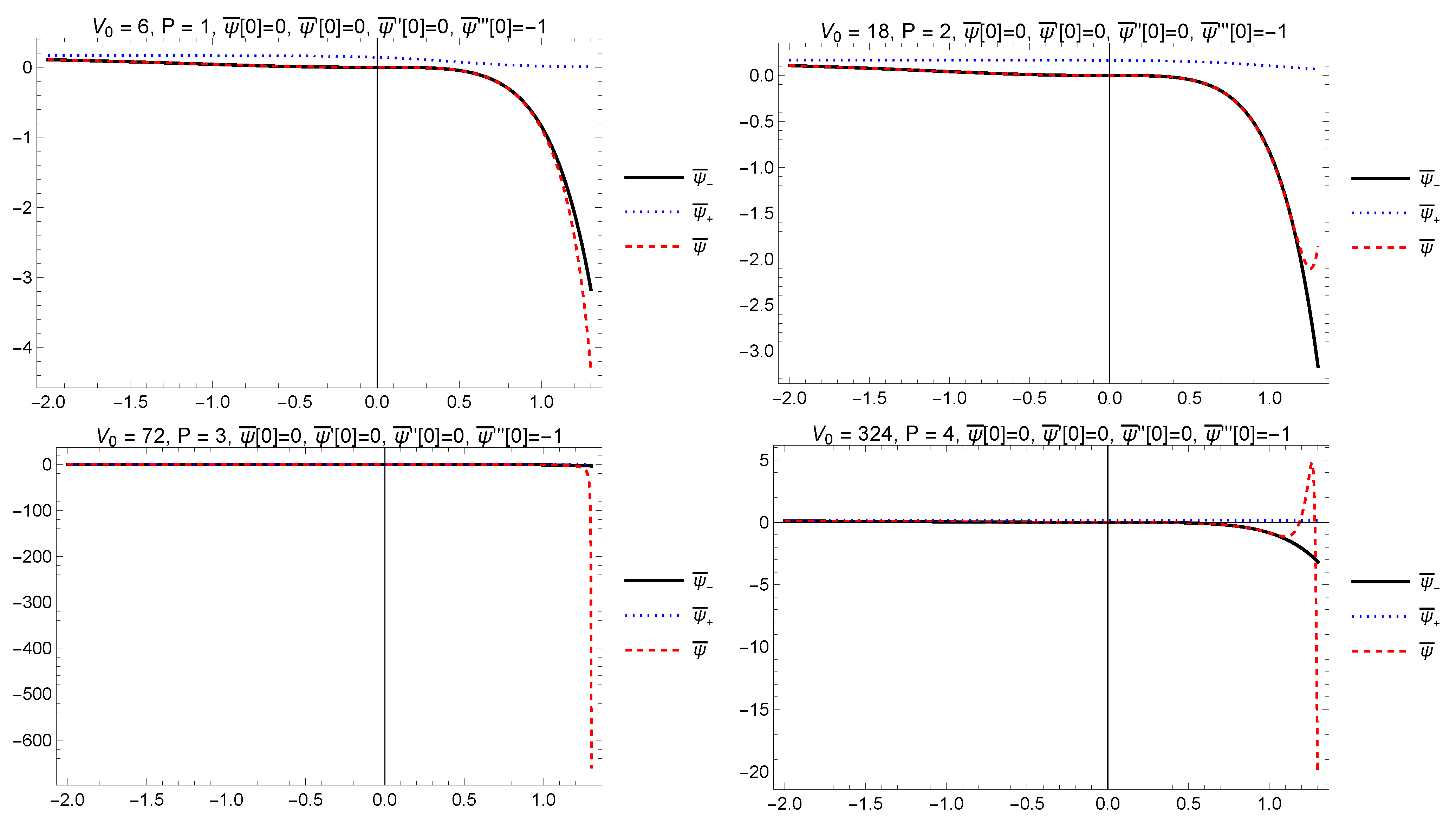
4.1. Power-Law Function $V\left(\mathrm{\Psi }\right)=V_0{\mathrm{\Psi }}^{P+1},P\ne 0$

For the power-law potential function, from the vector field $\left(4t{\partial }_t+x{\partial }_x-2\mathrm{\Phi }{\partial }_{\mathrm{\Phi }}-\frac{4}{P}\left(\mathrm{\Psi }{\partial }_{\mathrm{\Psi }}+\mathrm{\Phi }{\partial }_{\mathrm{\Phi }}\right)\right)$, we define the similarity transformation

$$\mathrm{\Psi }\left(t,x\right)=\psi \left(\sigma \right)t^{-\frac{1}{P}},\mathrm{\Phi }\left(t,x\right)=\varphi \left(\sigma \right)t^{-\frac{2+P}{2P}},\sigma \left(t,x\right)=\frac{x}{t^{\frac{1}{4}}},$$

and if $P\ne 0$, with reduced system

$$\begin{array}{ccc}\hfill \frac{{\partial }^2\varphi }{\partial {\sigma }^2}+V_0{\psi }^{P+1}-\frac{1}{4}\sigma \frac{\partial \psi }{\partial \sigma }-\frac{1}{P}\psi & =& 0,\hfill \end{array}$$

(27)

$$\begin{array}{ccc}\hfill \varphi -\frac{{\partial }^2\psi }{\partial {\sigma }^2}& =& 0.\hfill \end{array}$$

(28)

If $\varphi =0$, we have

$$\psi ={\psi }_1\sigma +{\psi }_0.$$

(29)

Then, from compatibility conditions, the only possible solution is the constant solution $\psi ={\psi }_0$, such that

$$V_0{\psi }_0^{P+1}-\frac{{\psi }_0}{P}=0\Rightarrow {\psi }_0={\left(P{V}_0\right)}^{-1/P}.$$

(30)

Therefore, we assume the non-trivial case $\varphi \ne 0$. Then, we have the fourth-order equation

$$\begin{array}{ccc}\hfill \frac{{\partial }^4\psi }{\partial {\sigma }^4}+V_0{\psi }^{P+1}-\frac{1}{4}\sigma \frac{\partial \psi }{\partial \sigma }-\frac{1}{P}\psi & =& 0.\hfill \end{array}$$

(31)

We introduce the logarithmic independent variable

$$\tau =ln\left(\sigma \right),$$

(32)

and redefine

$$\begin{array}{c}\hfill \psi \left(\sigma \right)=\overline{\psi }(ln\left(\sigma \right)).\end{array}$$

(33)

That is, for any function $f\left(\sigma \right)$, define

$$\overline{f}\left(\tau \right)=f\left(e^{\tau }\right).$$

(34)

Then, using the chain rule and the relation $\sigma =e^{\tau }$, we obtain

$$\begin{array}{cc}\hfill & \frac{\partial f}{\partial \sigma }=e^{-\tau }{\overline{f}}^{\prime }\left(\tau \right),\hfill \end{array}$$

(35)

$$\begin{array}{cc}\hfill & \frac{{\partial }^{2}f}{\partial {\sigma }^2}=e^{-2\tau }\left({\overline{f}}^{″}\left(\tau \right)-{\overline{f}}^{\prime }\left(\tau \right)\right),\hfill \end{array}$$

(36)

$$\begin{array}{cc}\hfill & \frac{{\partial }^3\psi }{\partial {\sigma }^3}=e^{-3\tau }\left({\overline{f}}^{\left(3\right)}\left(\tau \right)-3{\overline{f}}^{″}\left(\tau \right)+2{\overline{f}}^{\prime }\left(\tau \right)\right),\hfill \end{array}$$

(37)

$$\begin{array}{cc}\hfill & \frac{{\partial }^4\psi }{\partial {\sigma }^4}=e^{-4\tau }\left(u^{\left(4\right)}\left(\tau \right)-6u^{\left(3\right)}\left(\tau \right)+11u^{″}\left(\tau \right)-6u^{\prime }\left(\tau \right)\right).\hfill \end{array}$$

(38)

Then, (31) becomes

$$\begin{array}{cc}\hfill & \frac{\overline{\psi }\left(\tau \right)\left(P{V}_0\overline{\psi }{\left(\tau \right)}^P-1\right)}{P}+\left(-6e^{-4\tau }-\frac{1}{4}\right){\overline{\psi }}^{\prime }\left(\tau \right)+11e^{-4\tau }{\overline{\psi }}^{″}\left(\tau \right)-6e^{-4\tau }{\overline{\psi }}^{\left(3\right)}\left(\tau \right)+e^{-4\tau }{\overline{\psi }}^{\left(4\right)}\left(\tau \right)=0.\hfill \end{array}$$

(39)

Assuming that $\overline{\psi }$ is bounded with bounded derivatives as $\tau \to +\infty$, we obtain the asymptotic equation

$$\begin{array}{c}\hfill \frac{{\overline{\psi }}_{+}\left(\tau \right)\left(P{V}_0{\overline{\psi }}_{+}{\left(\tau \right)}^P-1\right)}{P}-\frac{1}{4}{\overline{\psi }}_{+}^{\prime }\left(\tau \right)=0,\end{array}$$

(40)

which admits the first integral

$$\begin{array}{c}\hfill c_1\frac{{\overline{\psi }}_{+}{\left(\tau \right)}^P}{\left(1-P{V}_0{\overline{\psi }}_{+}{\left(\tau \right)}^P\right)}=e^{-4\tau }\Rightarrow {\overline{\psi }}_{+}\left(\tau \right)=\left(P{V}_0+c_1{e}^{4\tau }\right){}^{-1/P}.\end{array}$$

(41)

Defining

$$z_{+}\left(\tau \right):=\frac{{\overline{\psi }}_{+}{\left(\tau \right)}^P}{\left(1-P{V}_0{\overline{\psi }}_{+}{\left(\tau \right)}^P\right)},$$

(42)

$z_{+}\left(\tau \right)$ is monotone decreasing as $\tau \to +\infty$ for $P>0$ and monotone increasing as $\tau \to +\infty$ for $P<0$. In other words, the asymptotic states of ${\overline{\psi }}_{+}\left(\tau \right)$ are

$$\begin{array}{cc}\hfill & \underset{\tau \to +\infty }{lim}{\overline{\psi }}_{+}\left(\tau \right)=0\mathrm{if}P>0,V_0>0,\hfill \end{array}$$

(43)

$$\begin{array}{cc}\hfill & \underset{\tau \to -\infty }{lim}{\overline{\psi }}_{+}\left(\tau \right)={\psi }_0:={\left(P{V}_0\right)}^{-1/P}\mathrm{if}P>0,V_0>0,\hfill \end{array}$$

(44)

and

$$\begin{array}{cc}\hfill & \underset{\tau \to +\infty }{lim}{\overline{\psi }}_{+}\left(\tau \right)={\psi }_0:={\left(P{V}_0\right)}^{-1/P}\mathrm{if}P<0,V_0<0,\hfill \end{array}$$

(45)

$$\begin{array}{cc}\hfill & \underset{\tau \to -\infty }{lim}{\overline{\psi }}_{+}\left(\tau \right)=0\mathrm{if}P>0,V_0>0.\hfill \end{array}$$

(46)

The cases of interest are as $\tau \to +\infty$. That is, the monotonic function $z_{+}$ unveils the asymptotic behaviour as $\tau \to +\infty$.

Now, assuming that $\overline{\psi }$ is bounded with bounded derivatives as $\tau \to -\infty$, we obtain the asymptotic equation

$$\begin{array}{cc}\hfill & -6{\overline{\psi }}_{-}^{\prime }\left(\tau \right)+11{\overline{\psi }}_{-}^{″}\left(\tau \right)-6{\overline{\psi }}_{-}^{\left(3\right)}\left(\tau \right)+{\overline{\psi }}_{-}^{\left(4\right)}\left(\tau \right)=0,\hfill \end{array}$$

(47)

with solution

$$\begin{array}{c}\hfill {\overline{\psi }}_{-}\left(\tau \right)=c_2{e}^{\tau }+\frac{1}{2}{c}_3{e}^{2\tau }+\frac{1}{3}{c}_4{e}^{3\tau }+c_5,\end{array}$$

(48)

such that

$$\underset{\tau \to -\infty }{lim}{\overline{\psi }}_{-}\left(\tau \right)=c_5.$$

(49)

Substituting $\psi \left(\tau \right)={\overline{\psi }}_{-}\left(\tau \right)$ in (39) and taking limit $\tau \to -\infty$, we obtain the compatibility condition

$$c_5\left(-1+P{V}_0{c}_5{}^P\right)=0.$$

(50)

That is, $c_5\in \left\{0,{\left(P{V}_0\right)}^{-1/P}\right\}.$ The choice $c_5={\left(P{V}_0\right)}^{-1/P}$ gives the proper matching condition

$$\underset{\tau \to -\infty }{lim}{\overline{\psi }}_{+}\left(\tau \right)=\underset{\tau \to -\infty }{lim}{\overline{\psi }}_{-}\left(\tau \right)={\left(P{V}_0\right)}^{-1/P}.$$

(51)

In summary, integrating from $\tau \to -\infty$ to $\tau >0$, we obtain that $\psi \left(\tau \right)\approx {\overline{\psi }}_{-}\left(\tau \right)$ for large $\tau$ close the boundary layer, whereas, integrating backwards from $\tau \to +\infty$ to $\tau <0$, we obtain that $\psi \left(\tau \right)\approx {\overline{\psi }}_{+}\left(\tau \right)$ as $\tau \to -\infty$. These results are illustrated in Figure 1.

Let us define the new time variable $s=(1+tanh(\tau \left)\right)/2$ that brings the interval $(-\infty ,\infty )$ to $(0,1)$. Then, the original layer problem becomes a two-point problem, with endpoints 0 and 1. The asymptotic solutions can be found as

$${\mathrm{\Phi }}_{-}\left(s\right)={\overline{\psi }}_{-}(-\mathrm{arctanh}(1-2s)),$$

(52)

that is,

$$\begin{array}{c}\hfill {\mathrm{\Phi }}_{-}\left(s\right)={\left(P{V}_0\right)}^{-1/P}+\frac{c_{3}s}{2-2s}+\left(c_2\left(\frac{1}{s}-1\right)+\frac{c_4}{3}\right)e^{-3\mathrm{arctanh}(1-2s)}.\end{array}$$

(53)

As $s\to 0^{+}$, we have the asymptotic behaviour ${\mathrm{\Phi }}_{-}\to {\left(P{V}_0\right)}^{-1/P}$.

Moreover,

$${\mathrm{\Phi }}_{+}\left(s\right)={\overline{\psi }}_{+}(-\mathrm{arctanh}(1-2s)),$$

(54)

becomes

$$\begin{array}{c}\hfill {\mathrm{\Phi }}_{+}\left(s\right)={\left(P{V}_0+\frac{c_1{s}^2}{{(1-s)}^2}\right)}^{-1/P},\end{array}$$

(55)

such that

$$\begin{array}{cc}\hfill & \underset{s\to 1^{-}}{lim}{\mathrm{\Phi }}_{+}\left(s\right)=0\mathrm{if}P>0,V_0>0.\hfill \end{array}$$

(56)

We have the matching condition

$$\underset{s\to 0^{+}}{lim}{\mathrm{\Phi }}_{-}\left(s\right)=\underset{s\to 0^{+}}{lim}{\mathrm{\Phi }}_{+}\left(s\right)={\left(P{V}_0\right)}^{-1/P}.$$

(57)

The next step is to introduce the stretched variables $\kappa =s/\epsilon$ and $\lambda =(1-s)/\epsilon$, and write a solution

$$\mathrm{\Phi }(s,\epsilon )=\zeta (\kappa ,\epsilon )+\eta (\lambda ,\epsilon )$$

(58)

where

$$\zeta \to {\left(P{V}_0\right)}^{-1/P}\mathrm{as}\kappa =s/\epsilon \to \infty$$

(59)

and

$$\eta \to 0\mathrm{as}\lambda =(1-s)/\epsilon \to \infty .$$

(60)

Near $s=0$, $\eta$ and its derivatives will be asymptotically negligible, so $d^j\mathrm{\Phi }(s,\epsilon )/d{s}^j\sim (1/{\epsilon }^j)\left[d^j\zeta (\kappa ,\epsilon )/d{\kappa }^j\right]$. Take, for example,

$${\zeta }_0(\kappa ,\epsilon )={\left(P{V}_0\right)}^{-1/P}+\frac{c_3\kappa \epsilon }{2-2\kappa \epsilon }+\left(c_2\left(\frac{1}{\kappa \epsilon }-1\right)+\frac{c_4}{3}\right)e^{-3\mathrm{arctanh}(1-2\kappa \epsilon )}.$$

(61)

Using the notation

$$\begin{array}{c}\hfill \overline{\psi }(\tau ,\epsilon )=\mathrm{\Phi }(\kappa ,\epsilon ),\kappa =\frac{tanh\left(\tau \right)+1}{2\epsilon }\end{array}$$

(62)

the approximated Equation (47) becomes

$$\begin{array}{cc}\hfill & 6\epsilon (4\kappa \epsilon (4\kappa \epsilon -3)+1){\mathrm{\Phi }}^{\prime }(\kappa ,\epsilon )\hfill \\ \hfill & +(\kappa \epsilon -1)[3(24\kappa \epsilon (2\kappa \epsilon -1)+1){\mathrm{\Phi }}^{″}(\kappa ,\epsilon )\hfill \\ \hfill & +4\kappa (\kappa \epsilon -1)\left(\kappa {\mathrm{\Phi }}^{\left(4\right)}(\kappa ,\epsilon )(\kappa \epsilon -1)+3{\mathrm{\Phi }}^{\left(3\right)}(\kappa ,\epsilon )(4\kappa \epsilon -1)\right)]=0,\hfill \end{array}$$

(63)

where primes mean derivatives with respect to $\kappa$, which admits the exact solution (61). Since we are taking $\epsilon$ as a small parameter, we see that the initial layer problem is of type

$$\begin{array}{cc}\hfill & \left(-3{\mathrm{\Phi }}^{″}\left(\kappa \right)-4\kappa \left(\kappa {\mathrm{\Phi }}^{\left(4\right)}\left(\kappa \right)+3{\mathrm{\Phi }}^{\left(3\right)}\left(\kappa \right)\right)\right)\hfill \\ \hfill & +\epsilon \left(6{\mathrm{\Phi }}^{\prime }\left(\kappa \right)+3\kappa \left(25{\mathrm{\Phi }}^{″}\left(\kappa \right)+4\kappa \left(\kappa {\mathrm{\Phi }}^{\left(4\right)}\left(\kappa \right)+6{\mathrm{\Phi }}^{\left(3\right)}\left(\kappa \right)\right)\right)\right)+O\left({\epsilon }^2\right)=0.\hfill \end{array}$$

(64)

Taking the expansion

$$\begin{array}{c}\hfill \mathrm{\Phi }\left(\kappa \right)={\mathrm{\Phi }}_0\left(\kappa \right)+\epsilon {\mathrm{\Phi }}_1\left(\kappa \right)+\dots \end{array}$$

(65)

we obtain at first-order

$$\begin{array}{c}\hfill -3{\mathrm{\Phi }}_0^{″}\left(\kappa \right)-4\kappa \left(\kappa {\mathrm{\Phi }}_0^{\left(4\right)}\left(\kappa \right)+3{\mathrm{\Phi }}_0^{\left(3\right)}\left(\kappa \right)\right)=0.\end{array}$$

(66)

Hence,

$${\mathrm{\Phi }}_0\left(\kappa \right)=\frac{4}{3}\sqrt{\kappa }(d_2\kappa -3d_1)+d_4\kappa +d_3.$$

(67)

At second-order, we have

$$60d_2\sqrt{\kappa }+6d_4-4{\kappa }^2{\mathrm{\Phi }}_1^{\left(4\right)}\left(\kappa \right)-12\kappa {\mathrm{\Phi }}_1^{\left(3\right)}\left(\kappa \right)-3{\mathrm{\Phi }}_1^{″}\left(\kappa \right)=0.$$

(68)

Hence,

$$\begin{array}{c}\hfill {\mathrm{\Phi }}_1\left(\kappa \right)=2d_2{\kappa }^{5/2}+\frac{4}{3}{d}_6{\kappa }^{3/2}+d_4{\kappa }^2+d_8\kappa -4d_5\sqrt{\kappa }+d_7,\end{array}$$

(69)

and so on. Finally, we replace the leading order and second-order terms (67) and (69), respectively, in (65) with the replacement (62).

Near $s=1$, $\zeta$ and its derivatives will be asymptotically negligible, so $d^j\mathrm{\Phi }(s,\epsilon )/d{s}^j\sim (1/{\epsilon }^j)\left[d^j\eta (\lambda ,\epsilon )/d{\lambda }^j\right]$. Take, for example,

$${\eta }_0(\lambda ,\epsilon )={\left(P{V}_0+c_1{e}^{4\mathrm{arctanh}(1-2\lambda \epsilon )}\right)}^{-1/P}.$$

(70)

Using the notation

$$\begin{array}{c}\hfill \overline{\psi }(\tau ,\epsilon )=\mathrm{\Phi }\left(\lambda \right),\lambda =\frac{1-tanh\left(\tau \right)}{2\epsilon },\end{array}$$

(71)

the approximated Equation (40), becomes

$$\begin{array}{c}\hfill 2V_0\mathrm{\Phi }{\left(\lambda \right)}^{P+1}+\lambda (1-\lambda \epsilon ){\mathrm{\Phi }}^{\prime }\left(\lambda \right)=\frac{2\mathrm{\Phi }\left(\lambda \right)}{P},\end{array}$$

(72)

which admits the solution (70).

Figure 1 shows the exact solution $\overline{\psi }$ of (39) with initial conditions $\overline{\psi }\left(0\right)=0,{\overline{\psi }}^{\prime }\left(0\right)=0,{\overline{\psi }}^{″}\left(0\right)=0,{\overline{\psi }}^{\left(3\right)}\left(0\right)=-1$ and the asymptotic solutions ${\overline{\psi }}_{-}=\frac{1}{6}-\frac{e^{\tau }}{2}+\frac{e^{2\tau }}{2}-\frac{e^{3\tau }}{6}$ and ${\overline{\psi }}_{+}={\left(6^P+e^{4\tau }\right)}^{-1/P}$ for $V_0=6^P/P,P>0$. This plot illustrates the accuracy of our analysis by selecting ${\overline{\psi }}_{-}$ as the inner solution for $\tau <{\tau }_0$, closing the boundary layer.

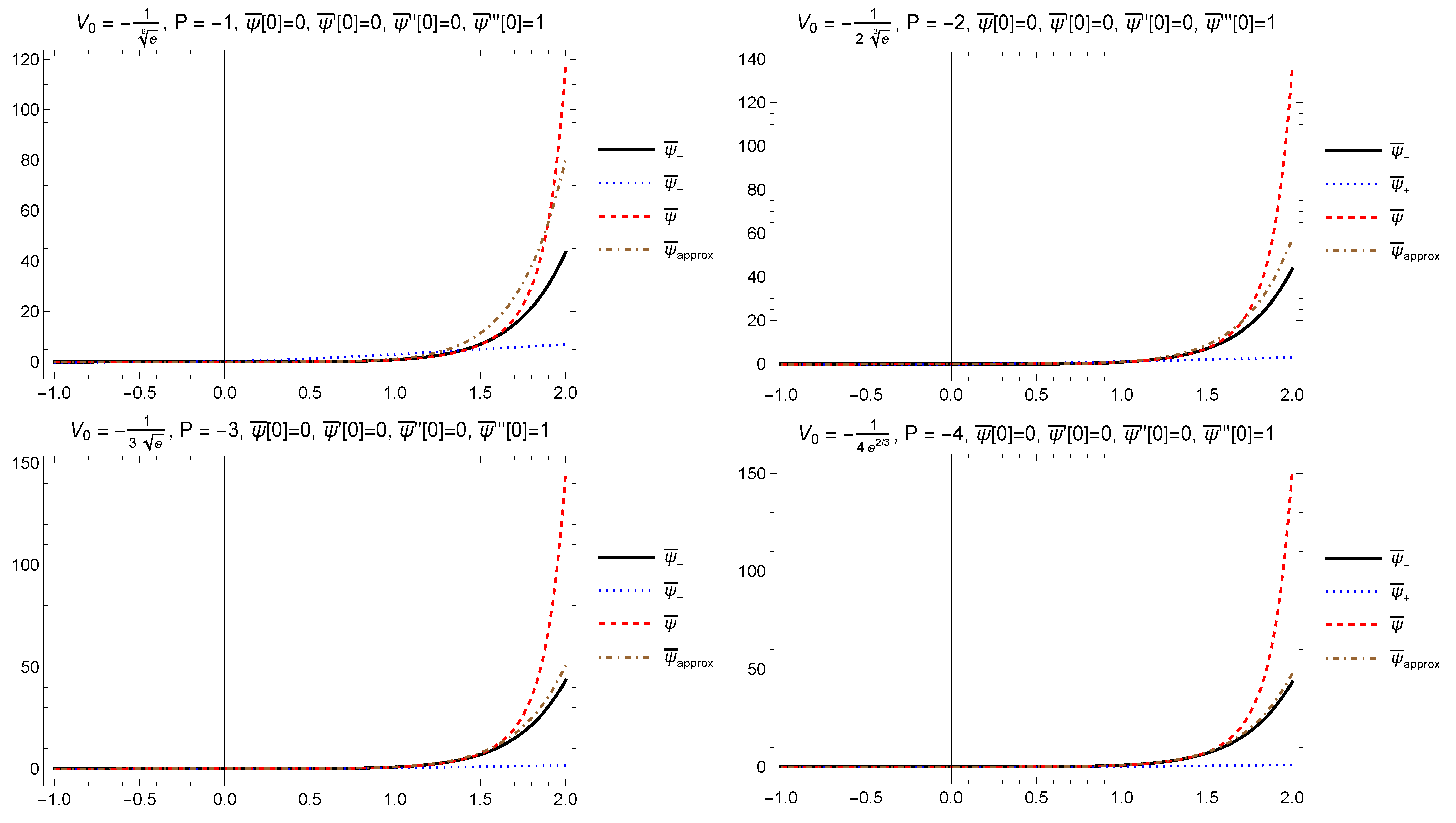
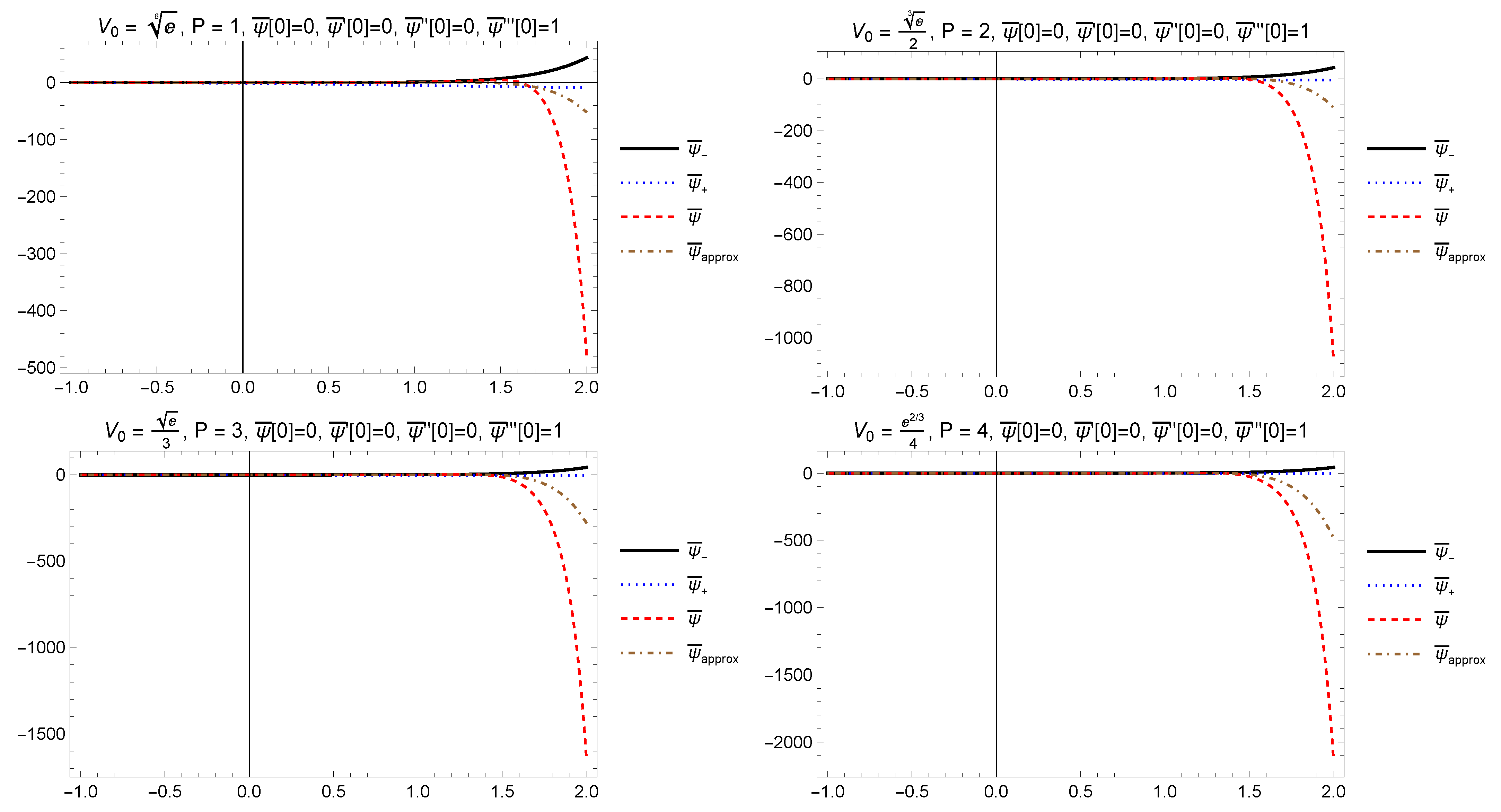
4.2. Exponential Function $V\left(\mathrm{\Psi }\right)=V_{0}exp\left(P\mathrm{\Psi }\right),P\ne 0$

On the other hand, for the exponential potential $V\left(\mathrm{\Psi }\right)=V_{0}exp\left(P\mathrm{\Psi }\right),P\ne 0$, the similarity transformation, which corresponds to the vector field $\left(4t{\partial }_t+x{\partial }_x-2\mathrm{\Phi }{\partial }_{\mathrm{\Phi }}-\frac{4}{P}\left({\partial }_{\mathrm{\Psi }}\right)\right)$, is

$$\mathrm{\Psi }\left(t,x\right)=\frac{lnt}{P}+\psi \left(\sigma \right),\mathrm{\Phi }=t^{-\frac{1}{2}}\varphi \left(\sigma \right),\sigma \left(t,x\right)=\frac{x}{t^{\frac{1}{4}}},$$

where the reduced system is

$$\begin{array}{ccc}\hfill \frac{{\partial }^2\varphi }{\partial {\sigma }^2}+V_0{e}^{P\psi }-\frac{1}{P}-\frac{1}{4}\sigma \frac{\partial \psi }{\partial \sigma }& =& 0,\hfill \end{array}$$

(73)

$$\begin{array}{ccc}\hfill \varphi -\frac{{\partial }^2\psi }{\partial {\sigma }^2}& =& 0.\hfill \end{array}$$

(74)

We introduce the logarithmic independent variable (32) and define $\psi \left(\sigma \right)$ by (33). Then, using the chain rule and the relation $\sigma =e^{\tau }$, we obtain

$$V_0{e}^{P\overline{\psi }\left(\tau \right)}+\left(-6e^{-4\tau }-\frac{1}{4}\right){\overline{\psi }}^{\prime }\left(\tau \right)+11e^{-4\tau }{\overline{\psi }}^{″}\left(\tau \right)-6e^{-4\tau }{\overline{\psi }}^{\left(3\right)}\left(\tau \right)+e^{-4\tau }{\overline{\psi }}^{\left(4\right)}\left(\tau \right)-\frac{1}{P}=0.$$

(75)

Assuming that $\overline{\psi }$ is bounded with bounded derivatives as $\tau \to +\infty$, we obtain the asymptotic equation

$$\begin{array}{c}\hfill V_0{e}^{P{\overline{\psi }}_{+}\left(\tau \right)}-\frac{1}{P}-\frac{1}{4}{\overline{\psi }}_{+}^{\prime }\left(\tau \right)=0,\end{array}$$

(76)

with solution

$${\overline{\psi }}_{+}\left(\tau \right)=ln\left(\left(P{V}_0+e^{4\tau +c_{1}P}\right){}^{-1/P}\right).$$

(77)

Assuming that $\overline{\psi }$ and $V_0{e}^{P\overline{\psi }\left(\tau \right)}$ are bounded with bounded derivatives as $\tau \to -\infty$, we obtain, as in Section 4.1, the asymptotic Equation (47), with solution (48). Substituting $\psi \left(\tau \right)={\overline{\psi }}_{-}\left(\tau \right)$ in (75), and taking limit $\tau \to -\infty$, we obtain

$$-\frac{1}{P}+V_0{e}^{c_{5}P}=0\Rightarrow c_5=ln\left[{\left(P{V}_0\right)}^{-1/P}\right].$$

(78)

That is, we have the matching condition

$$\underset{\tau \to -\infty }{lim}{\overline{\psi }}_{+}\left(\tau \right)=\underset{\tau \to -\infty }{lim}{\overline{\psi }}_{-}\left(\tau \right)=ln\left[{\left(P{V}_0\right)}^{-1/P}\right].$$

(79)

As in Section 4.1, integrating from $\tau \to -\infty$ to $\tau >0$, we obtain that $\psi \left(\tau \right)\approx {\overline{\psi }}_{-}\left(\tau \right)$ for large $\tau$, whereas, integrating backwards from $\tau \to +\infty$ to $\tau <0$, we obtain that $\psi \left(\tau \right)\approx {\overline{\psi }}_{+}\left(\tau \right)$ as $\tau \to -\infty$. These results are illustrated in Figure 2 and Figure 3. Nevertheless, when the term $V_0{e}^{P\overline{\psi }\left(\tau \right)}$ in (75) is not negligible, the approximation of $\overline{\psi }$ by the solution of the asymptotic Equation (47) is not accurate as $\tau \to +\infty$. Then, the asymptotic Equation (47) is replaced by

$$\begin{array}{c}\hfill V_0{e}^{P\psi \left(\tau \right)+4\tau }+{\psi }^{\left(4\right)}\left(\tau \right)-6{\psi }^{\left(3\right)}\left(\tau \right)+11{\psi }^{″}\left(\tau \right)-6{\psi }^{\prime }\left(\tau \right)=0,\end{array}$$

(80)

which cannot be solved analytically.

Using the same method, we define the new time variable $s=(1+tanh(\tau \left)\right)/2$ that brings the interval $(-\infty ,\infty )$ to $(0,1)$. Then, the original layer problem becomes a two-point problem, with endpoints 0 and 1. The asymptotic solutions can be found as

$$\begin{array}{c}\hfill {\mathrm{\Phi }}_{-}\left(s\right)=ln\left[{\left(P{V}_0\right)}^{-1/P}\right]+\frac{c_{3}s}{2-2s}+\left(c_2\left(\frac{1}{s}-1\right)+\frac{c_4}{3}\right)e^{-3\mathrm{arctanh}(1-2s)}.\end{array}$$

(81)

As $s\to 0^{+}$, we have the asymptotic behaviour $e^{{\mathrm{\Phi }}_{-}}\to {\left(P{V}_0\right)}^{-1/P}$.

Similarly, we have

$$\begin{array}{c}\hfill e^{{\mathrm{\Phi }}_{+}\left(s\right)}={\left(P{V}_0+\frac{c_1{s}^2}{{(1-s)}^2}\right)}^{-1/P},\end{array}$$

(82)

such that

$$\begin{array}{cc}\hfill & \underset{s\to 1^{-}}{lim}{e}^{{\mathrm{\Phi }}_{+}\left(s\right)}=0\mathrm{if}P>0,V_0>0.\hfill \end{array}$$

(83)

Finally, by introducing the stretched variables $\kappa =s/\epsilon$ and $\lambda =(1-s)/\epsilon$, we write a solution

$$\mathrm{\Phi }(s,\epsilon )=\zeta (\kappa ,\epsilon )+\eta (\lambda ,\epsilon ),$$

(84)

where

$$\zeta \to ln\left[{\left(P{V}_0\right)}^{-1/P}\right]\mathrm{as}\kappa =s/\epsilon \to \infty ,$$

(85)

and

$$\eta \to 0\mathrm{as}\lambda =(1-s)/\epsilon \to \infty .$$

(86)

Then, the layer problem becomes a two-point problem, with endpoints 0 and 1, and we obtain the asymptotic solutions following similar approaches as in Section 4.1.

Figure 2 shows the exact solution $\overline{\psi }$ of (75) with initial conditions $\overline{\psi }\left(0\right)=0,{\overline{\psi }}^{\prime }\left(0\right)=0,{\overline{\psi }}^{″}\left(0\right)=0,{\overline{\psi }}^{\left(3\right)}\left(0\right)=1$ and the asymptotic solutions ${\overline{\psi }}_{-}=\frac{e^{\tau }}{2}-\frac{e^{2\tau }}{2}+\frac{e^{3\tau }}{6}-\frac{1}{6}$ and ${\overline{\psi }}_{+}=-\frac{ln\left(e^{P+4\tau }+e^{P/6}\right)}{P}$ for $V_0=\frac{e^{P/6}}{P},P<0$. In this example, the approximations are accurate.

Figure 3 shows the exact solution $\overline{\psi }$ of (75) with the same initial conditions, and the asymptotic solutions ${\overline{\psi }}_{\pm }$ for $V_0=\frac{e^{P/6}}{P},P>0$. The approximation of $\overline{\psi }$ by the solution of the asymptotic Equation (47) is not accurate as $\tau \to +\infty$. Then, the asymptotic Equation (47) is replaced by (80). The numerical solution ${\overline{\psi }}_{approx}$ of (80) is represented by a dot-dashed line in Figure 2 and Figure 3.

5. Conclusions

Lie symmetry analysis is a powerful method for analysing nonlinear differential equations. In this study, the Lie symmetry analysis was applied to solve the group classification problem for a $1+n$-dimensional nonlinear higher-order Schrödinger equation inspired by GUP. The partial differential equation of our analysis admits an arbitrary potential function, which was a constraint according to the admitted Lie point symmetries. For an arbitrary potential function, we found that the admitted Lie symmetries are the Killing vectors of the n-dimensional space in addition to the vector field ${\partial }_t$. However, a new symmetry vector presented in Theorems 1 and 2 can be found for specific function forms of the potential function. To demonstrate the application of the Lie symmetry vectors, we used the corresponding Lie invariants to define similarity transformations and reduce the partial-differential equation into an ordinary differential equation. Because of the nonlinearity of the reduced equation, we studied the asymptotic dynamics and evolution.

Concerning asymptotic analysis, we have obtained asymptotic solutions

$$\begin{array}{cc}\hfill {\overline{\psi }}_{-}\left(\tau \right)& =c_2{e}^{\tau }+\frac{1}{2}{c}_3{e}^{2\tau }+\frac{1}{3}{c}_4{e}^{3\tau }+\left\{\begin{array}{cc}{\left(P{V}_0\right)}^{-1/P}& \mathrm{power}-\mathrm{law}\mathrm{function}\\ ln\left[{\left(P{V}_0\right)}^{-1/P}\right]& \mathrm{exponential}\mathrm{function}\end{array}\right.,\hfill \\ \hfill {\overline{\psi }}_{+}\left(\tau \right)& =\left\{\begin{array}{cc}\left(P{V}_0+c_1{e}^{4\tau }\right){}^{-1/P}& \mathrm{power}-\mathrm{law}\mathrm{function}\\ ln\left(\left(P{V}_0+e^{4\tau +c_{1}P}\right){}^{-1/P}\right)& \mathrm{exponential}\mathrm{function}\end{array}\right.,\hfill \end{array}$$

with the proper matching condition

$$\underset{\tau \to -\infty }{lim}{\overline{\psi }}_{+}\left(\tau \right)=\underset{\tau \to -\infty }{lim}{\overline{\psi }}_{-}\left(\tau \right)=\left\{\begin{array}{cc}{\left(P{V}_0\right)}^{-1/P}& \mathrm{power}-\mathrm{law}\mathrm{function}\\ ln\left[{\left(P{V}_0\right)}^{-1/P}\right]& \mathrm{exponential}\mathrm{function}\end{array}\right..$$

For the power-law potential, it is confirmed numerically that as $\tau \to -\infty$, $\psi \left(\tau \right)\approx {\overline{\psi }}_{+}\left(\tau \right)$, whereas, for large $\tau$, $\psi \left(\tau \right)\approx {\overline{\psi }}_{-}\left(\tau \right)$. However, in the exponential case, when the term $V_0{e}^{P\overline{\psi }\left(\tau \right)}$ is not negligible, the approximation by ${\overline{\psi }}_{-}\left(\tau \right)$ is not accurate as the boundary layer is approached and has to be replaced by ${\overline{\psi }}_{approx}\left(\tau \right)$.

Finally, the layer problem becomes a two-point problem, with endpoints 0 and 1 by introducing the stretched variables $\kappa =s/\epsilon$ and $\lambda =(1-s)/\epsilon$, and writing a formal solution

$$\mathrm{\Phi }(s,\epsilon )=\zeta (\kappa ,\epsilon )+\eta (\lambda ,\epsilon ),$$

(87)

where

$$\zeta \to \left\{\begin{array}{cc}{\left(P{V}_0\right)}^{-1/P}& \mathrm{power}-\mathrm{law}\mathrm{function}\\ ln\left[{\left(P{V}_0\right)}^{-1/P}\right]& \mathrm{exponential}\mathrm{function}\end{array}\right.,\mathrm{as}\kappa =s/\epsilon \to \infty ,$$

(88)

and

$$\eta \to 0\mathrm{as}\lambda =(1-s)/\epsilon \to \infty .$$

(89)

Then, it is interesting to analyse possible asymptotic solutions for different initial/ boundary conditions, but this numerical treatment is out of the scope of the present research. In general, when solving the problem of approximating a function ${\psi }_{\epsilon }\left(\tau \right)$ depending on a small parameter $\epsilon$ in a domain D, the algorithm presented in [53] can be applied.

This work contributes to the subject of the application of Lie point symmetries on nonlinear differential equations. In this study, we considered a Schrödinger equation constructed by the deformation algebra of the quadratic GUP. However, that is not the unique proposed GUP, and other deformations algebras exist. Therefore, in future work, we plan to perform a detailed classification of the higher-order Schrödinger equations for different models of GUP. Finally, we will present formal expansions, representing valid asymptotic approximations of the function ${\psi }_{\epsilon }\left(\tau \right)$ for other initial conditions that we set out to study by singular perturbation methods, boundary layers, and multiple time scales.

References

1. Stephani, H. Differential Equations: Their Solutions Using Symmetry; Cambridge University Press: New York, NY, USA, 1989. [Google Scholar]
2. Bluman, G.W.; Kumei, S. Symmetries of Differential Equations; Springer: New York, NY, USA, 1989. [Google Scholar]
3. Leach, P.G.L.; Gorringe, V.M. A conserved Laplace-Runge-Lenz-like vector for a class of three-dimensional motions. Phys. Lett. A 1988, 133, 289. [Google Scholar]
4. Gazinov, R.K.; Ibragimov, N.H. Lie Symmetry Analysis of Differential Equations in Finance. Nonlinear Dyn. 1998, 17, 387. [Google Scholar]
5. Ibragimov, N.H. On the group classification of second order differential equations. (Russ.) Dokl. Akad. Nauk SSSR 1968, 183, 274. [Google Scholar]
6. Azad, H.; Mustafa, M.T. Symmetry analysis of wave equation on sphere. J. Math. Anal. Appl. 2007, 333, 1180. [Google Scholar]
7. Tsamparlis, M.; Paliathanasis, A. Two-dimensional dynamical systems which admit Lie and Noether symmetries. J. Phys. A Math.Theor. 2011, 44, 175202. [Google Scholar]
8. Mahomed, F.M. Symmetry group classification of ordinary differential equations: Survey of some results. Math. Methods Appl. Sci. 2007, 30, 1995. [Google Scholar]
9. Jamal, S.; Kara, A.H.; Bokhari, Ȧ.H. Symmetries, conservation laws, reductions, and exact solutions for the Klein–Gordon equation in de Sitter space–times. Can. J. Phys. 2012, 90, 667. [Google Scholar]
10. Halder, A.K.; Paliathanasis, A.; Rangasamy, S.; Leach, P.G.L. Similarity solutions for the complex Burgers’ hierarchy. Z. Naturforschung A 2019, 74, 597. [Google Scholar]
11. Jamal, S.; Kara, A.H. New higher-order conservation laws of some classes of wave and Gordon-type equations. Nonlinear Dyn. 2012, 67, 97. [Google Scholar]
12. Chesnokov, A.A. Symmetries and exact solutions of the rotating shallow-water equations. J. Appl. Mech. Techn. Phys. 2008, 49, 737. [Google Scholar]
13. Jamal, S. Solutions of quasi-geostrophic turbulence in multi-layered configurations. Quaest. Math. 2018, 41, 409. [Google Scholar]
14. Halder, A.K.; Paliathanasis, A.; Leach, P.G.L. Noether’s Theorem and Symmetry. Symmetry 2018, 10, 744. [Google Scholar]
15. Schwarz, F. Solving second order ordinary differential equations with maximal symmetry group. Computing 1999, 62, 1. [Google Scholar]
16. Reid, G.J.; Wittkopf, A.D. Determination of maximal symmetry groups of classes of differential equations. In ISSAC ’00: Proceedings of the 2000 International Symposium on Symbolic and Algebraic Computation; Association for Computing Machinery: New York, NY, USA, 2000; pp. 272–280. [Google Scholar]
17. Ali, S.; Safdar, M.; Qadir, A. Linearization from complex Lie point transformations. J. Appl. Math. 2014, 2014, 793247. [Google Scholar]
18. Karpman, V.I. Lyapunov approach to the soliton stability in highly dispersive systems. I. Fourth order nonlinear Schrödinger equations. Phys. Lett. A 1996, 215, 254. [Google Scholar]
19. Karpman, V.I.; Shagalov, A.G. Stability of solitons described by nonlinear Schrödinger-type equations with higher-order dispersion. Phys. D 2000, 144, 194. [Google Scholar]
20. Segata, J. Factorization technique for the fourth-order nonlinear Schrödinger equation. Math. Methods Appl. Sci. 2006, 26, 1785. [Google Scholar]
21. Pausader, B. The cubic fourth-order Schrödinger equation. J. Funct. Anal. 2009, 256, 2473. [Google Scholar]
22. Pausader, B.; Shao, S. The mass-critical fourth-order Schrödinger equation in high dimensions. J. Hyperbolic Differ. 2010, 7, 651. [Google Scholar]
23. Baquet, C.; Villamizar-Roa, E.J. On the management fourth-order Schrodinger-Hartree equation. Evol. Equ. Control 2020, 9, 865. [Google Scholar]
24. Liu, X.; Zhang, T. The Cauchy problem for the fourth-order Schrödinger equation in Hs. J. Math. Phys. 2021, 62, 071501. [Google Scholar]
25. Erdogan, B.; Green, W.R.; Torpak, E. On the fourth order Schrödinger equation in three dimensions: Dispersive estimates and zero energy resonances. J. Differ. Equ. 2021, 271, 152. [Google Scholar]
26. Fibich, G.; Ilan, B.; Papanicolaou, G. Self-focusing with fourth-order dispersion. SIAM J. Appl. Math. 2002, 62, 1437. [Google Scholar]
27. Fibich, G.; Ilan, B.; Schochet, S. Critical exponents and collapse of nonlinear Schrödinger equations with anisotropic fourth-order dispersion. Nonlinearity 2003, 16, 1809. [Google Scholar]
28. Karpman, V.I. Envelope solitons in gyrotropic media. Phys. Rev. Lett. 1995, 74, 2455. [Google Scholar]
29. Quarshi, M.M.A.; Yusuf, A.; Aliyu, A.I.; Inc, M. Optical and other solitons for the fourth-order dispersive nonlinear Schrödinger equation with dual-power law nonlinearity. Superlattices Microstruct. 2017, 105, 183. [Google Scholar]
30. Fedele, R.; Schamel, H.; Shukla, P.K. Solitons in the Madelung’s Fluid. Phys. Scr. 2002, 2002, 18. [Google Scholar]
31. Natali, F.; Pastor, A. The Fourth-Order Dispersive Nonlinear Schrödinger Equation: Orbital Stability of a Standing Wave. SIAM J. Appl. Dyn. Syst. 2015, 14, 1326–1347. [Google Scholar] [CrossRef]
32. Hayaski, N.; Naumkin, P.I. On the inhomogeneous fourth-order nonlinear Schrödinger equation. J. Math. Phys. 2015, 56, 093502. [Google Scholar]
33. Konishi, K.; Paffuti, G.; Provero, P. Minimum physical length and the generalized uncertainty principle in string theory. Phys. Lett. B 1990, 234, 276. [Google Scholar]
34. Camelia, A. Relativity in spacetimes with short-distance structure governed by an observer-independent (Planckian) length scale. Int.J. Mod. Phys. D 2002, 11, 35. [Google Scholar]
35. Martinetti, P.; Mercati, F.; Tomassini, L. Minimal length in quantum space and integrations of the line element in noncommutative geometry. Rev. Math. Phys. 2012, 24, 1250010. [Google Scholar]
36. Ashtekar, A.; Lewandowski, J. Background independent quantum gravity: A status report. Class. Quantum Grav. 2004, 21, R53. [Google Scholar]
37. Maggiore, M. A generalized uncertainty principle in quantum gravity. Phys. Lett. B 1993, 304, 65. [Google Scholar]
38. Hossenfelder, S. Minimal length scale scenarios for quantum gravity. Living Rev. Relativ. 2013, 16, 2. [Google Scholar]
39. Das, S.; Vagenas, E.C. Universality of quantum gravity corrections. Phys. Rev. Lett. 2008, 101, 221301. [Google Scholar]
40. Moayedi, S.K.; Setare, M.R.; Moayeri, H. Quantum gravitational corrections to the real klein-gordon field in the presence of a minimal length. Int. J. Theor. Phys. 2010, 49, 2080. [Google Scholar]
41. Hamil, B.; Merad, M.; Birkandan, T. Applications of the extended uncertainty principle in AdS and dS spaces. Eur Phys. J. Plus 2019, 134, 278. [Google Scholar]
42. Dabrowski, M.P.; Wagner, F. Asymptotic generalized extended uncertainty principle. EPJC 2020, 80, 676. [Google Scholar]
43. Nenmeli, V.; Shankaranarayanan, S.; Todorinov, V.; Das, S. Maximal momentum GUP leads to quadratic gravity. Phys. Lett. B 2021, 821, 136621. [Google Scholar]
44. Das, A.; Das, S.; Vagenas, E.C. Discreteness of space from GUP in strong gravitational fields. Phys. Lett. B 2020, 809, 135772. [Google Scholar]
45. Aghababaei, S.; Mordpour, H.; Vagenas, E.C. Hubble tension bounds the GUP and EUP parameters. Eur. Phys. J. Plus 2021, 136, 997. [Google Scholar]
46. Ovsiannikov, L.V. Group Analysis of Differential Equations; Academic Press: New York, NY, USA, 1982. [Google Scholar]
47. Zhang, Z.-Y.; Li, G.-F. Lie symmetry analysis and exact solutions of the time-fractional biological population model. Phys. A 2020, 540, 123134. [Google Scholar]
48. Jamal, S.; Kara, A.H.; Narain, R. Wave equations in Bianchi Space-times. J. App. Math. 2012, 2012, 765361. [Google Scholar]
49. Lahno, V.; Zhdanov, R.; Magda, O. Group classification and exact solutions of nonlinear wave equations. Acta Appl. Math. 2006, 91, 253. [Google Scholar]
50. Baikov, V.A.; Gladkov, A.V.; Wiltshire, R.J. Lie symmetry classification analysis for nonlinear coupled diffusion. J. Phys. A Math. Gen. 1998, 31, 7483. [Google Scholar]
51. Huang, D.; Ivanova, N.M. Group analysis and exact solutions of a class of variable coefficient nonlinear telegraph equations. J. Math. Phys. 2007, 48, 073507. [Google Scholar]
52. Cherniha, R.; Serov, M.; Prystavka, Y. A complete Lie symmetry classification of a class of (1+2)-dimensional reaction-diffusion-convection equations. Commun. Nonlinear Sci. Numer. Simul. 2021, 92, 105466. [Google Scholar]
53. Verhulst, F. Methods and Applications of Singular Perturbations: Boundary Layers and Multiple Timescale Dynamics, Texts in Applied Mathematics; Springer: New York, NY, USA, 2005. [Google Scholar] [CrossRef]
54. Paliathanasis, A.; Tsamparlis, M. Lie and Noether point symmetries of a class of quasilinear systems of second-order differential equations. J. Geom. Phys. 2016, 107, 45. [Google Scholar]
55. Karpathopoulos, L.; Paliathanasis, A.; Tsamparlis, M. Lie and Noether point symmetries for a class of nonautonomous dynamical systems. J. Math. Phys. 2017, 58, 082301. [Google Scholar]
56. Paliathanasis, A.; Tsamparlis, M. The geometric origin of Lie point symmetries of the Schrödinger and the Klein–Gordon equations. Int. J. Geom. Meth. Mod. Phys. 2014, 11, 1450037. [Google Scholar]
Figure 1. Comparison of exact solution ψ ¯ of (39) with initial conditions ψ ¯ ( 0 ) = 0 , ψ ¯ ( 0 ) = 0 , ψ ¯ ( 0 ) = 0 , ψ ¯ ( 3 ) ( 0 ) = 1 and the asymptotic solutions ψ ¯ ± for V 0 = 6 P / P , P > 0 .
Mathematics 10 03204 g001
Figure 2. Comparison of exact solution ψ ¯ of (75) with initial conditions ψ ¯ ( 0 ) = 0 , ψ ¯ ( 0 ) = 0 , ψ ¯ ( 0 ) = 0 , ψ ¯ ( 3 ) ( 0 ) = 1 and the asymptotic solutions ψ ¯ ± for V 0 = e P / 6 P , P < 0 .
Mathematics 10 03204 g002
Figure 3. Comparison of exact solution ψ ¯ of (39) with initial conditions ψ ¯ ( 0 ) = 0 , ψ ¯ ( 0 ) = 0 , ψ ¯ ( 0 ) = 0 , ψ ¯ ( 3 ) ( 0 ) = 1 and the asymptotic solutions ψ ¯ ± for V 0 = e P / 6 P , P > 0 .
Mathematics 10 03204 g003
Publisher’s Note: MDPI stays neutral with regard to jurisdictional claims in published maps and institutional affiliations.