Forecasting the Volatility of Cryptocurrencies in the Presence of COVID-19 with the State Space Model and Kalman Filter

Abstract

During the COVID-19 pandemic, cryptocurrency prices showed abnormal volatility that attracted the participation of many investors. Studying the behaviour of volatility for the prices of cryptocurrency is an interesting problem to be investigated. This research implements the state space model framework for volatility incorporating the Kalman filter. This method directly forecasts the conditional volatility of five cryptocurrency prices (Bitcoin (BTC), Ethereum (ETH), Ripple (XRP), Litecoin (LTC) and Bitcoin Cash (BCH)) for 10,000 consecutive hours, i.e., approximately 417 days during the COVID-19 pandemic from 26 February 2020, 00:00 h until 18 April 2021, 00:00 h. The performance of this model is compared to the GARCH (1,1) model and the neural network autoregressive (NNAR) based on root mean square error (RMSE), mean absolute error (MAE) and the volatility plot. The autocorrelation function plot, histogram and the residuals plot are used to examine the model adequacy. Among the three models, the state space model gives the best fit. The state space model gives the narrowest confidence interval of volatility and value-at-risk forecasts among the three models.

1. Introduction

Cryptocurrency is a form of digital currency that is neither upheld nor maintained by any single body or organization. Instead, ownership and transaction information are kept in a blockchain-based distributed ledger [1,2]. Blockchain, which was first developed for Bitcoin [3] and is currently the base technology of many cryptocurrencies, is a decentralized transaction and data management technology [4].

The principles behind blockchain technology are discussed in detail by [5]. According to [6], the blockchain technology has been actively applied in five main sectors such as finance, Internet of Things (IoT), public and social service, reputation system as well as security and privacy. In the financial sector, this technology is applied to the peer-to-peer financial market [7] and postal operator (PO) service [8]. The new e-business model by [9] and the privacy-preserving method for commissioning an IoT device into a cloud ecosystem by [10] are examples of application in the IoT sector domain. Meanwhile, in the public and social services sector, the blockchain technology has been widely applied for land registration [11], energy saving [12] and education [13,14].

Cryptocurrency can be used to perform transactions of goods and services entirely online and is not connected to any government or central bank. Since the introduction of the first cryptocurrency, Bitcoin, by [3], the cryptocurrency market has constantly been the centre of attention for investors. Cryptocurrency transactions involve fund transfers between two parties without the intervention of a third party such as banks or credit and debit cards. Payments made using cryptocurrency are safe and secure as the private key is only known to the owner of the wallet. It also requires minimal processing fees which makes it cheaper than most online transactions. For traders and investors, the cryptocurrency market is always open for trading unlike the stock market which is opened during specific hours and is closed during weekends or public holidays. On the other hand, the use of cryptocurrency is limited as it is not widely used in many countries around the world. Payments made are also irreversible and it is prone to be used in illegal activities such as money laundering and tax evasion due to its lack of transparency in transactions [15,16].

The coronavirus COVID-19 outbreak which made the cryptocurrency market [17,18,19] unpredictable, causing abnormal volatility in the prices of cryptocurrency that attracted many investors. The unpredictable behaviour during the COVID-19 outbreak sparked interest in studying the volatility of cryptocurrency. Predicting volatility is essential in measuring the risk of a security. Common statistical measures of financial risks include volatility and value-at-risk (VaR) [20].

The autoregressive conditional heteroskedasticity (ARCH) model [21] and the general ARCH (GARCH) model [22] measure volatility based on the square root of the conditional variance. The GARCH model led to some innovations in modelling financial volatility such as the smooth transition GARCH(ST-GARCH) model [23] which models the asymmetric volatility in cryptocurrency and the hybrid deep learning model which incorporates the long short-term memory-artificial neural network (LSTM-ANN) model. An instance where the LSTM-ANN model networks with the GARCH model to observe copper-price volatility forecast is available in [24]. Several extensions of the GARCH model with stochastic volatility models in modelling the volatility of cryptocurrencies such as Bitcoin and Litecoin were examined by [25].

The GARCH (1,1) model is the simplest variation of the GARCH model and is used in modelling variance. This model has been widely applied due to its ergodicity and strong stationarity of the conditional variance (squared volatility) of the process [26]. The Markov time scale of returns and volatilities for most financial data is equal to 1 [27].

In recent years, machine learning models especially the ANN model, have been widely implemented in financial risk forecasting due to their nature of modelling based on the historical data itself, giving higher forecast accuracy compared to existing time series models measuring volatility [28,29,30,31]. The neural network (NN) volatility predictive model framework based on the neural network autoregressive (NNAR) model by [32] to forecast financial risk measures was more effective than the GARCH (1,1) and the Heston-Nandi (HN)-GARCH (1,1) models were introduced by [33].

The state space model is a type of probabilistic graphical model that describes the dependency between the observed variable and its hidden state variable [34]. Kalman filter is the most commonly used optimal algorithm for the state space model framework which was introduced by [35]. This method is used mainly in the field of engineering. Recent research in quantitative finance have incorporated the Kalman filter algorithm due to its ability to separate hidden noises from the observations and hence gives forecasts with higher accuracy. Several examples include the Kalman filter-based hybridization model by [36] in forecasting exchange rates. The proposed hybrid model (PHM) by [37] to forecast crude oil prices also uses the Kalman filter approach to determine the time-varying weight for the proposed hybrid combination model of exponential smoothing model (ESM), ARIMA and NNAR.

The state space model using the Kalman filtering algorithm to model volatility was introduced by [38]. However, this model is only constructed considering the autoregressive (AR) process in the hidden state variable. The extension of the model by [38] considering the moving average (MA) process, in addition to the AR process, for a more general analysis was done by [39]. The modification between the ideas of [38,39] produces the state space model variation known as the state space ARIMA model which is mainly used for time series data. Several studies that use the state space ARIMA model include forecasting of consumer retail data [40], the supply chain data [41] and the sugarcane yield data [42].

So far, no study used the state space ARIMA model by incorporating Kalman filters to directly forecast the conditional volatility. The Kalman filter possesses good dynamic real-time tracking characteristics, especially in volatile data such as cryptocurrency and stock market data.

This paper implements the state space ARIMA model which incorporates the Kalman filtering algorithm to forecast the conditional volatility of five cryptocurrency prices (Bitcoin (BTC), Ethereum (ETH), Ripple (XRP), Litecoin (LTC) and Bitcoin Cash (BCH)) for 10,000 consecutive hours, i.e., approximately 417 days during the COVID-19 pandemic from 26 February 2020, 00:00 h until 18 April 2021, 00:00 h. The forecast accuracy of the model is then compared with the GARCH (1,1) model and the NNAR model [32]. The GARCH (1,1) model forecasts the conditional volatility based on the square root of the conditional variance while the NNAR model forecasts the conditional volatility without denoising. Hence, these models were chosen to be compared with the state space ARIMA model to forecast conditional volatility by denoising using Kalman filtering. The confidence intervals of volatility and VaR forecasts for the selected level of confidence of these three models are also computed.

The remaining part of this paper is organized as follows: Section 2 discusses the methodology used, Section 3 gives a brief discussion of the data used, Section 4 discusses the results and Section 5 concludes.

2. Materials and Methods

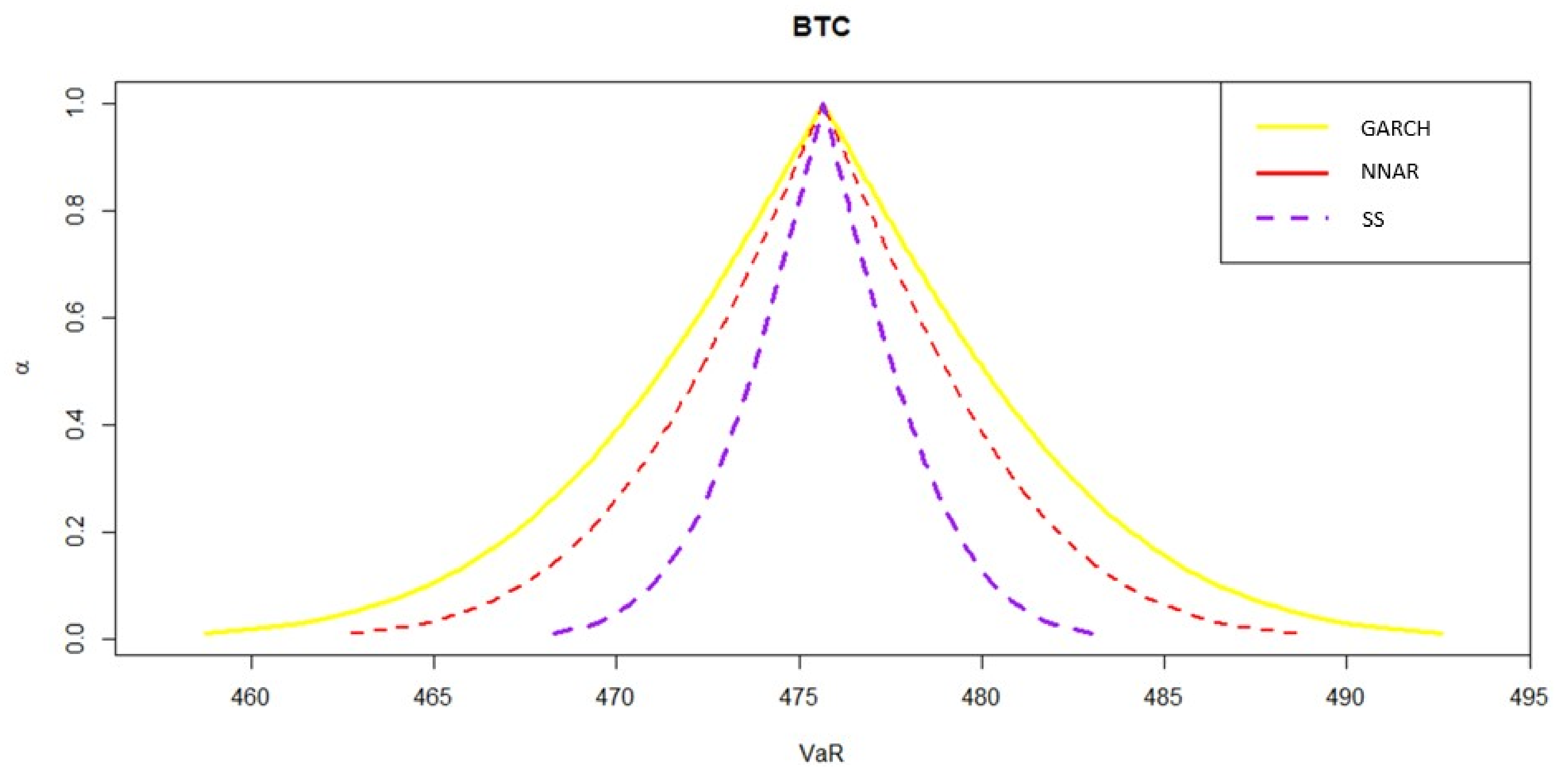
2.1. Forecasting VaR

According to [43], the one-step-ahead forecast of the VaR for centred log-returns $r_t$ with tail probability $p$ is obtained by using

$${\mathrm{VaR}}_{t+1} \left(p\right)=-{\sigma }_{t+1} F_r^{-1} \left(p\right),$$

(1)

where ${\sigma }_{t+1}$ is the forecast of the volatility and $F_r^{-1}\left(p\right)$ is the inverse of the cumulative density function of log-returns evaluated at the confidence level $p$.

From (1), it can be seen that forecasting the VaR is equivalent to forecasting the volatility. The volatility forecasts from 3 different forecasting models: the GARCH (1,1) model, the NN volatility predictive model and the state space volatility model using the Kalman filtering algorithm are then compared using error measures such as the root mean square error (RMSE) and mean absolute error (MAE) that can be computed as follows

$$\mathrm{RMSE}=\sqrt{\frac{1}{N}{\displaystyle \sum }_{i=1}^N{\left(x_i-{\widehat{x}}_i\right)}^2}$$

$$\mathrm{MAE}=\frac{1}{N}{\displaystyle \sum }_{i=1}^N\left|x_i-{\widehat{x}}_i\right|$$

where $x_i$ is the actual volatility and ${\widehat{x}}_i$ is the one-step ahead forecasted volatility produced by the GARCH (1,1), the NNAR and the state space (SS) models. Lower RMSE and MAE indicate higher accuracy of model forecasts.

2.2. The GARCH (1,1) Model

The autoregressive conditional heteroskedasticity (ARCH) model by [21] was extended by [22] to model the conditional variance, ${\sigma }^2$ of a time series. This model uses values of the past squared observations and past variances to model the variance at time $t$. For a time series, $X_t$, the GARCH $(1,1$) model for conditional variance is given by

$$X_t=e_t{\sigma }_t$$

$${\sigma }_t^2=\omega +{\alpha }_1{r}_{t-1}^2+{\beta }_1{\sigma }_{t-1}^2,$$

(2)

where $e_t~N\left(0,1\right)$ is white noise.

The centred log return which is given by

$$r_t^{\ast }=\frac{r_t-\overline{r}}{\rho },$$

(3)

is considered as $X_t$ in (2) where $r_t$ is the log return, $\overline{r}$ is the mean of $r_t$ and $\rho =\frac{\mathrm{mean} \mathrm{of} r_t-\overline{r}}{\mathrm{standard} \mathrm{deviation} \mathrm{of} r_t}.$

The volatility is then obtained by taking the square root of the conditional variance, ${\sigma }_t^2$ from (2).

To forecast the volatility of cryptocurrency in the context of this work, the centred log return of cryptocurrency prices, $r_t^{\ast }$ is fit with ARMA (0,0) for the mean, GARCH (1,1) model for the variance and the distribution used for the conditional density is the student—t distribution. The conditional volatility is then calculated by taking the square root of the conditional variance forecasts. Finally, the accuracy of the model is evaluated using error measures such as RMSE and MAE.

The rugarch package [44] was used to aid the fitting of the GARCH (1,1) model.

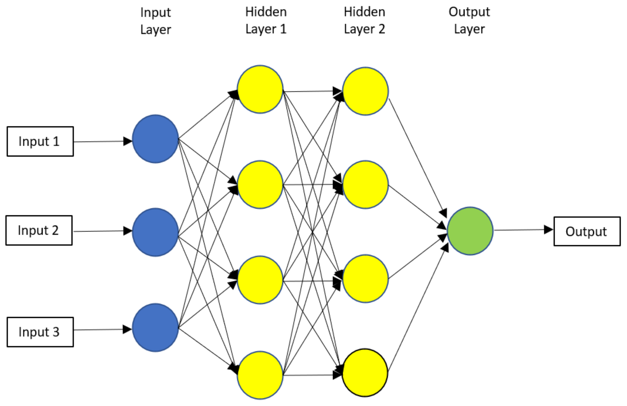
2.3. The NN Autoregressive (NNAR) Model

The neural network (NN) model is a type of machine learning model that is capable of modelling complex nonlinear relationships without any prior knowledge of the underlying relationship. For this model, several hidden layers are added between the input layer and the output layer (Figure 1). Each hidden layer contains a set of nodes where each node undergoes a nonlinear transformation of its input before being transferred to the next layer [45].

A special version of the neural network model for time series which is called the neural network autoregression or NNAR model was introduced by [32]. In contrast to the GARCH model which computes volatility as the square root of the conditional variance, [33] directly models the volatility of a stock using a single hidden layer feed-forward NN volatility model which is based on the NNAR ($p,P,k)$ model.

An NNAR ($p,P,k)$ model has $p$ lagged inputs, $P$ seasonal lagged inputs and $k$ nodes in one hidden layer. The number of input nodes or time series lags of the NN model can be decided from the order of the auto-regressive (AR) process.

To forecast the volatility of cryptocurrencies using the NNAR ($p,P,k)$ model in the context of this work, the $p$ lagged values of the centered absolute value of log returns of cryptocurrencies $\left|r_{t-1}^{\ast }\right|, \left|r_{t-2}^{\ast }\right|, \left|r_{t-3}^{\ast }\right|,\dots , \left|r_{t-p}^{\ast }\right|$ of the target variable $\left|r_t^{\ast }\right|$, for $r_t^{\ast }$ in (3), are fit to the input layer.

There are five hidden units in hidden layer 1,

$${\alpha }_l=g({\omega }_{l0}^{\left(1\right)}+{{\displaystyle \sum }}_{j=1}^p{\omega }_{lj}^{\left(1\right)}\left|r_{t-j}^{\ast }\right|)$$

(4)

where ${\omega }_{l0}^{\left(1\right)}$ is the intercept terms, or bias, $g$ is the sigmoid function $g\left(t\right)=\frac{1}{1+e^{-t}}$, and ${\omega }_{lj}^{\left(1\right)}$ is the weights parameter.

The transition from layer $k-1$ to $k$ is then modelled as:

$$z_l^{\left(k\right)}={\omega }_{l0}^{\left(k-1\right)}+{\displaystyle \sum }_{j=1}^{p_{k-1}}{\omega }_{lj}^{\left(k-1\right)}{a}_j^{\left(k-1\right)}$$

where $a_l^{\left(k\right)}=g^k\left(z_l^{\left(k\right)}\right)$ is the generalisation of (4) for $k$ nodes.

$\left|r_{t-1}^{\ast }\right|,\left|r_{t-2}^{\ast }\right|, \left|r_{t-3}^{\ast }\right|,\dots , \left|r_{t-p}^{\ast }\right|$ are fit to the NNAR $\left(p,P,k\right)$ model and the value of $k=\frac{\left(p+P+1\right)}{2}$, rounded to the nearest integer, is automatically selected [46]. The fit of the model is then evaluated using RMSE and MAE.

The forecasting approach of this model is recursive such that the parameters are re-estimated by remodelling the historical inputs with every new observation introduced. This process is repeated iteratively until all the forecast values are computed. For obtaining one-step ahead forecasts, the available historical input is set as the training data.

The forecast package [46] was used to aid the fitting of the NNAR model.

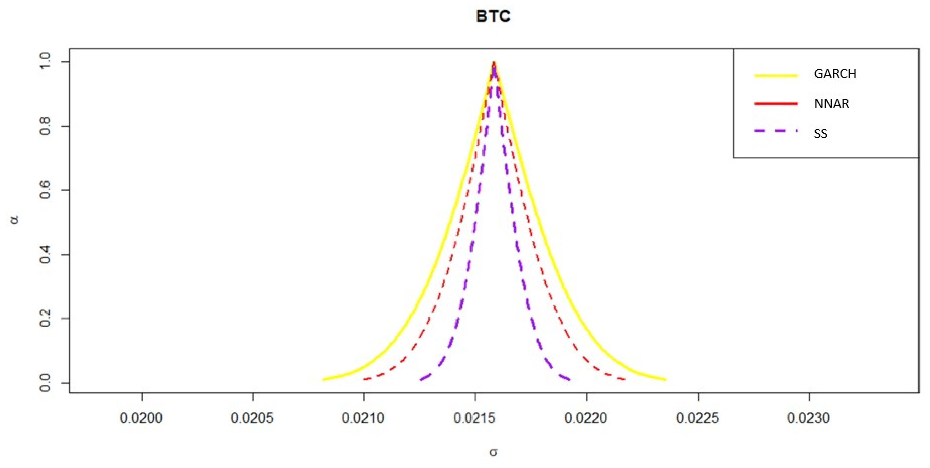
2.4. The State Space (SS) Model Based on the Kalman Filtering Algorithm for Volatility

2.4.1. Gaussian SS Model

Let $y_t$ be an observation at time $t$ and ${\alpha }_t$ be the latent state process for $y_t$ at time $t$ for discrete time intervals $t=1,\dots ,n$.

$y_t$ and ${\alpha }_t$ can be written as a linear Gaussian state space model where

$$y_t=Z{\alpha }_t+{\epsilon }_t (\mathrm{observation} \mathrm{equation})$$

$${\alpha }_{t+1}=T{\alpha }_t+R{\eta }_t, (\mathrm{state} \mathrm{equation})$$

(5)

where ${\epsilon }_t~N\left(0,H\right)$, ${\eta }_t~N\left(0,Q\right)$ and ${\alpha }_1~N\left(a_1,P_1\right)$ are independent of each other and system matrices $Z$, $T$, and $R$, and covariance matrices $H$, and $Q$ are time invariant.

As shown by [39], the one-step-ahead forecast of the state, ${\widehat{\alpha }}_{t+1}=\mathrm{E}({\alpha }_{t+1}| y_t,\dots , y_1)$ with variances, $P_{t+1}=\mathrm{var}({\alpha }_{t+1}|y_t,\dots , y_1)$ and error, $v_t$ can be obtained by the following Kalman recursions:

$${\nu }_t=y_t-Z{a}_t,$$

$$F_t=\mathrm{var}\left({\nu }_t\right)=Z{P}_t{Z}^T+H,$$

$$K_t=P_t{Z}^{\mathrm{T}},$$

$${\widehat{\alpha }}_{t+1}=T\left(a_t+K_t{F}_t^{-1}{v}_t\right),$$

$$P_{t+1}=T\left(P_t-K_t{F}_t^{-1}{K}_t^{\mathrm{T}}\right)T^{\mathrm{T}}+RQR.$$

The detailed derivation of this algorithm can be found in [47].

2.4.2. The ARIMA SS Model

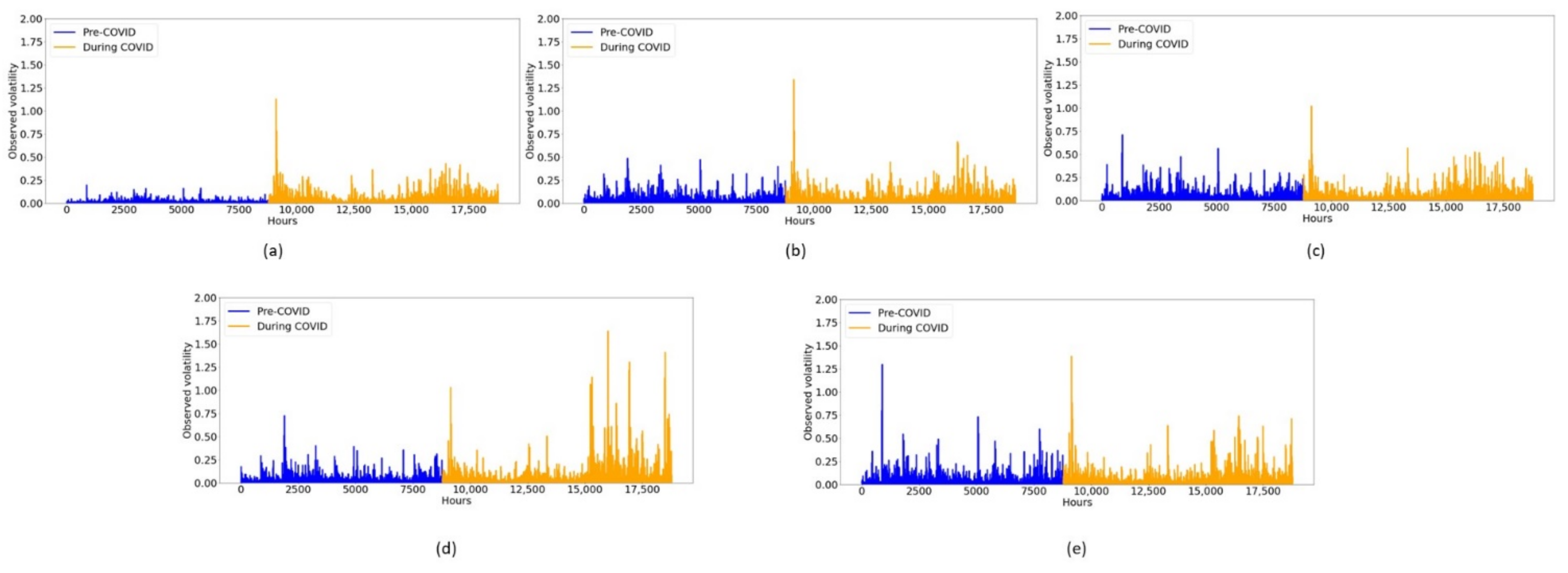
Let $y_t^{\ast }={\mathsf{\Delta }}^d{y}_t$ be the differenced values of $y_t$ such that it follows a univariate ARIMA ($p,d,q$) model which can be written as

$$y_t^{\ast }={\varphi }_1{y}_{t-1}^{\ast }+\cdots +{\varphi }_p{y}_{t-p}^{\ast }+{\xi }_t+{\theta }_1{\xi }_{t-1}+\cdots +{\theta }_q{\xi }_{t-q},$$

(6)

where ${\xi }_t~N\left(0, {\sigma }^2\right)$.

Let $r=\max \left(p,q+1\right)$.

From (5), let the log of returns of cryptocurrencies be the observations, $y_t$ and the conditional volatility be the states, ${\alpha }_{t+1}$. Then, the forecast of volatility can be computed by using the Kalman filtering method with parameters:

$$\begin{gathered} Z^{\mathrm{T}}=\left(\begin{array}{c}{1}_{d+1}\\ 0\\ ⋮\\ 0\end{array}\right) H=0, T=\left(\begin{array}{ccccc}{U}_d& 1_d^{\mathrm{T}}& 0& \dots & 0\\ 0& {\varphi }_1& 1& \dots & 0\\ ⋮& ⋮& ⋮& \ddots & ⋮\\ ⋮& {\varphi }_{r-1}& 0& \dots & 1\\ 0& {\varphi }_r& 0& \dots & 0\end{array}\right), R=\left(\begin{array}{c}{0}_d\\ 1\\ {\theta }_1\\ ⋮\\ {\theta }_{r-1}\end{array}\right), \\ {\alpha }_t=\left(\begin{array}{c}{y}_{t-1}\\ ⋮\\ {\mathsf{\Delta }}^{d-1}{y}_{t-1}\\ y_t^{\ast }\\ {\varphi }_2{y}_{t-1}^{\ast }+\cdots +{\varphi }_r{y}_{t-r+1}^{\ast }+{\theta }_1{\eta }_t+\cdots +{\theta }_{r-1}{\eta }_{t-r+2}\\ ⋮\\ {\varphi }_r{y}_{t-1}^{\ast }+{\theta }_{r-1}{\eta }_t\end{array}\right), Q={\sigma }^2, \end{gathered}$$

$$a_1=\left(\begin{array}{c}0\\ ⋮\\ 0\end{array}\right), P_{\ast ,1}=\left(\begin{array}{cc}0& 0\\ 0& S_r\end{array}\right), P_{\infty ,1}=\left(\begin{array}{cc}{I}_d& 0\\ 0& 0\end{array}\right), {\eta }_t={\xi }_{t+1},$$

(7)

where ${\varphi }_{p+1}=\cdots ={\varphi }_r={\theta }_{q+1}=\cdots ={\theta }_{r-1}=0,$ $1_{d+1}$ is a $1\times \left(d+1\right)$ vector of ones, $U_d$ is $d\times d$ upper triangular matrix of ones and $S_r$ is covariance matrix of stationary elements of ${\alpha }_1$.

The elements of initial state vector ${\alpha }_1$, which correspond to the differenced values $y_0,\dots , {\mathsf{\Delta }}^{d-1}{y}_0$ are treated as diffuse. $P_{\ast ,1}$ contains the covariance of the nondiffuse elements of ${\alpha }_1$ and $P_{\infty ,1}$ and is a diagonal matrix with ones on those diagonal elements which relate to the diffuse elements of ${\alpha }_1.$ $S_r$ can be calculated by solving linear equation $\left(I-T\otimes T\right)\mathrm{vec}\left(S_r\right)=\mathrm{vec}\left(R{R}^{\mathrm{T}}\right)$ [47].

The steps in fitting the SS ARIMA model for volatility forecasting are as follows:

Step 1: The log return of a cryptocurrency is fitted to get the $AR\left(p\right)$, differences, $d$ and $MA\left(q\right)$ coefficients for the best ARIMA model in (6). The parameters ($p,d,q$) are obtained by using the Hyndman–Khandakar algorithm in [46]. In this algorithm, the number of differences $0\le d\le 2$ is determined using the repeated Kwiatkowski–Phillips–Schmidt–Shin (KPSS) test [48]. The values of $p$ and $q$ are then chosen by minimising the Akaike Information Criterion (AIC) after differencing the data $d$ times.

Step 2: A state space model is fit to the data. The centred absolute value of the log of returns, $\left|r_t^{\ast }\right|$ is set up set as the state equation at time $t$ and the corresponding observation equation with the coefficients obtained in step 1 is set up.

Step 3: Kalman filtering is then applied to obtain the one-step-ahead forecast of the conditional volatility. The fit of the model is then evaluated using RMSE and MAE.

The KFAS package [47] was used to aid the fitting of the SS model.

3. Data Description

The five cryptocurrencies analysed in this work are Bitcoin (BTC), Ethereum (ETH), Ripple (XRP), Litecoin (LTC) and Bitcoin Cash (BCH). The details on each cryptocurrency are given in

Table 1. Details on the cryptocurrencies selected which is used in this study.

Cryptocurrency	Initial Release Date	Original Author	Usage
Bitcoin (BTC)	9 January 2009	Satoshi Nakamoto [3]	Largest cryptocurrency in the world. Alternative to currencies.
Ethereum (ETH)	30 July 2015	Vitalik Buterin & Gavin Wood [51]	Coin value is referred to as Ether which is the native token to Ethereum that can be used as an alternative to currencies. Ethereum makes it possible for creating and running applications, smart contracts etc. on the network [52].
Litecoin (LTC)	9 October 2011	Charlie Lee [53]	Peer-to-peer internet currency with instant transactions and near-zero cost payments to anyone in the world [54].
Ripple (XRP)	June 2012	David Schwartz, Jed McCaleb, & Arthur Britto	Digital payment network and protocol [55].
Bitcoin Cash (BCH)	August 2017	Bitcoin Cash is a fork of Bitcoin	Electronic cash payment system.

.

The hourly data of the price of selected cryptocurrencies for 10,000 h which is approximately 417 days during the COVID-19 pandemic period, i.e., from 26 February 2020, 00:00 h until 18 April 2021, 00:00 h was used. The data were retrieved from the CryptoDataDownload website, https://www.cryptodatadownload.com (accessed on 15 July 2021).

According to [49], these five cryptocurrencies were listed among the top 10 cryptocurrencies with the highest market cap in January 2020. However, the market efficiency behaviour of the major traded cryptocurrencies changed following the COVID-19 outbreak in March 2020 [50]. Hence, the volatility forecasts of these cryptocurrencies during this period were investigated. To visualise the changes in the volatility behaviour during the COVID-19 and pre-COVID-19 (from 25 February 2019, 00:00 h until 25 February 2020, 00:00 h) periods, the observed volatility plots (Figure 2) were obtained for the cryptocurrencies investigated. These plots show that the pandemic had an effect on the volatility. Hence, it was of interest to model the volatility during the COVID-19 period.

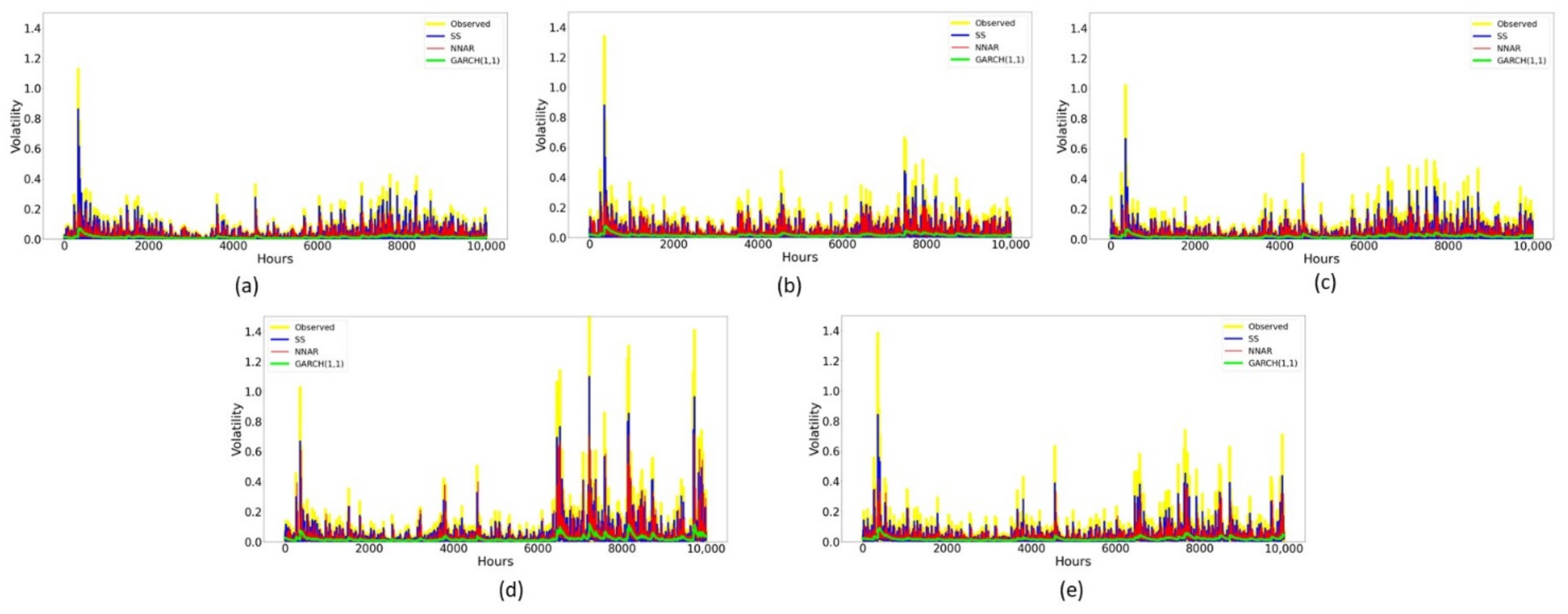
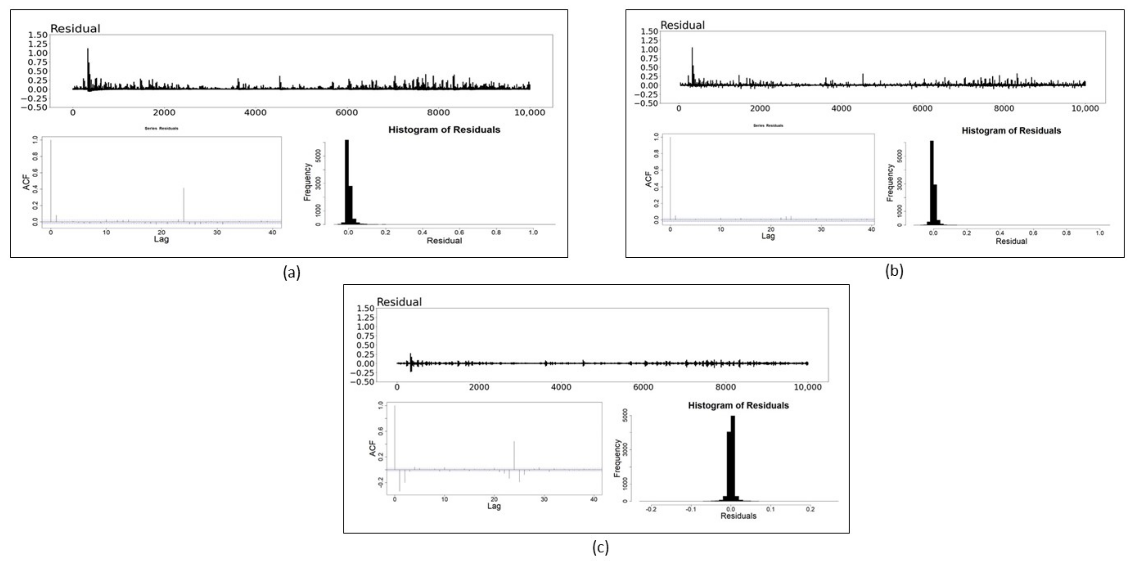
4. Results and Discussion

The GARCH (1,1), the NNAR [32] and the SS models based on the Kalman filtering algorithm were fit to estimate the volatility forecasts of BTC, ETH, LTC, XRP and BCH for the given period. The descriptive statistics of the log return of the aforementioned cryptocurrencies are given in

Table 2. Descriptive statistics for log return of BTC, ETH, LTC, XRP and BCH.

Dataset	Maximum	Minimum	Mean	Median	Standard Deviation	Skewness	Kurtosis	NNAR	ARIMA
BTC	1	−0.49492	0.000189	−0.00014	0.015105	−3.47787	174.4704	(39,0,20)	(5,1,1)
ETH	1	−0.61396	0.000233	−0.00021	0.018783	−2.75487	163.5906	(39,0,20)	(5,2,0)
LTC	1	−0.49576	0.000155	−0.00011	0.019459	−1.26584	81.98503	(32,0,16)	(5,2,0)
XRP	1	−0.66014	0.000201	0	0.025944	2.698127	152.0154	(35,0,18)	(5,2,0)
BCH	1	−0.61638	0.000132	−0.0000866	0.020892	−2.55303	140.3643	(28,0,14)	(1,1,2)

. The optimal value of parameters $\left(p,P,k\right)$ for the NNAR model that are obtained according to the Akaike Information Criterion (AIC) and the ARIMA parameters $\left(p,d,q\right)$ for the SS model are also shown in Table 2. The NNAR model requires more parameters compared to the SS ARIMA model. Furthermore, the SS ARIMA model is faster in terms of computational speed. The skewness values in Table 2 indicate that all five cryptocurrencies are heavily skewed where BTC, ETH, LTC and BCH are skewed to the left while XRP is skewed to the right. The large values of kurtosis for all five cryptocurrencies indicate that they are heavily tailed.

The RMSE and MAE of each model for all five datasets are shown in

Table 3. RMSE and MAE of predicted volatility of BTC, ETH, LTC, XRP and BCH ¹.

MODEL	BTC		ETH		LTC		XRP		BCH
	RMSE	MAE	RMSE	MAE	RMSE	MAE	RMSE	MAE	RMSE	MAE
GARCH (1,1)	0.0299	0.0116	0.0354	0.0144	0.0340	0.0147	0.0562	0.0192	0.0409	0.0162
NNAR	0.0227	0.0099	0.0257	0.0121	0.0265	0.0130	0.0393	0.0169	0.0334	0.0149
SS	0.0109	0.0046	0.0155	0.0070	0.0150	0.0072	0.0248	0.0096	0.0182	0.0077

¹ Lowest RMSE and MAE values for each dataset are bolded.

, and it can clearly be seen that the SS model produces forecasts with the highest accuracy compared to the other two models.

Figure 3 shows the estimated volatility forecasts of the five cryptocurrencies for the three models. Large spikes in the volatility plots are present for all other four cryptocurrencies besides XRP. These spikes appear to be outliers at the beginning phase. The highest peak of volatility for these data are $\sigma >1$ for BTC, LTC and BCH and $\sigma >1.2$ for ETH. The highest volatility spike for XRP is $\sigma >1.5$ between time 6000 and 8000. The SS model and the NNAR model managed to capture almost all the spikes. However, the SS volatility approximation appears to be closer to the observed values at the highest peak as mentioned earlier. On the other hand, the GARCH (1,1) model failed to capture any of the spikes and appears flat most of the time. This observation is consistent with the results in Table 3 where the GARCH (1,1) model produces forecasts with large errors while the SS model produces forecasts with smallest errors across all five datasets.

The residuals plot, autocorrelation function (ACF) plot and histogram of the estimated volatility are shown in Figure 4, Figure 5, Figure 6, Figure 7 and Figure 8. From the histogram, only the residuals of the SS model are approximately symmetrical while the residuals of the NNAR model and the GARCH (1,1) model are both skewed to the right. In the residual versus time plot, the residuals of the SS model are also more evenly spread around the centre, 0 compared to its counterparts. The outliers in the volatility plots near time 0 are also reflected in the residual plots. In addition, the ACF plots for all models suggest that the residuals are not distinguishable from a white noise series.

The SS model used for volatility forecasting is a two-stage forecasting method where the log return is first fit into an ARIMA model and then the one-step ahead forecasts of the volatility are directly obtained by the Kalman filtering algorithm. Through this method, the unnecessary noises are also filtered out. This filtering improves the forecasting ability of the model. Forecasting the volatility is a challenging process since it is not directly observable. The GARCH (1,1) model is a conditional variance forecast model which means that volatility can only be computed by taking the square root of the forecasted variance. This might cause occurrences of errors in forecast since the volatility is not directly forecasted. On the other hand, the NNAR model only directly forecasts the conditional volatility without considering noise filtering. Hence in this situation, the SS model outperforms the GARCH (1,1) model and the NNAR model.

The one-step ahead VaR and volatility forecasts for all three models for BTC are also computed along with their confidence intervals with $\alpha =0.01$ level of significance, as shown in Figure 9 and Figure 10, respectively. The confidence intervals of the VaR and volatility forecasts for all five datasets show similar behaviour (refer to the Supplementary Materials for the confidence interval plots for ETH, LTC, XRP and BCH). It can be clearly seen that the SS model produces the smallest ranges for confidence intervals involving the VaR and volatility forecasts while the GARCH (1,1) model produces the largest ranges. Models that produce VaR and volatility forecasts with smaller variability i.e., confidence interval with smallest range, enable risk managers to make more precise statements about VaR. Therefore, the SS model is recommended for VaR and volatility forecasting.

5. Conclusions

This work implements the SS model framework by incorporating Kalman filter to directly forecast the conditional volatility of the prices of five cryptocurrencies (BTC, ETH, XRP, LTC and BCH) for a selected 10,000-consecutive hour period during the COVID-19 pandemic. This model gives the best forecast accuracy when compared to the NNAR model and the GARCH (1,1) model. The confidence interval of the SS model is the narrowest among these three models. The SS model produces estimates of volatility and VaR forecasts with smallest variability. This will enable us to make more precise statements about VaR. The SS model considers the hidden noise in the prices of cryptocurrencies when forecasting conditional volatility which makes it surpass the NNAR model [37] and the GARCH (1,1) model.

The study of volatility modelling is crucial especially for portfolio optimisations, hedging and pricing of derivative securities [56]. For investors who wish to integrate cryptocurrencies in their investment portfolio, the level of return volatility has been viewed as an important attribute of cryptocurrencies [25]. A positive return-volatility connection of the cryptocurrencies may suggest its potential hedging and safe-haven features which differ from other traditional financial assets; thus investors would resort to transferring volatility and uncertainty to cryptocurrency markets in times of financial turmoil [23]. The results from this work may add weight to modelling volatility of cryptocurrencies. By incorporating Kalman filter in the SS ARIMA model, unnecessary noise can be filtered during the forecasting process, thus increasing the accuracy of the forecasts which leads to more accurate predictions of volatility.

References

1. Milutinović, M. Cryptocurrency. Ekonomika 2018, 64, 105–122. [Google Scholar] [CrossRef]
2. Pernice, I.G.A.; Scott, B. Cryptocurrency. Internet Policy Rev. 2021, 10, 1–5. [Google Scholar] [CrossRef]
3. Nakamoto, S. Bitcoin: A peer-to-peer electronic cash system. Decentralized Bus. Rev. 2008, 21260, 1–9. [Google Scholar]
4. Yli-Huumo, J.; Ko, D.; Choi, S.; Park, S.; Smolander, K. Where is current research on blockchain technology?—A systematic review. PLoS ONE 2016, 11, e0163477. [Google Scholar] [CrossRef] [PubMed]
5. Pilkington, M. Blockchain technology: Principles and applications. In Research Handbook on Digital Transformations; Edward Elgar Publishing: London, UK, 2016. [Google Scholar]
6. Zheng, Z.; Xie, S.; Dai, H.-N.; Chen, X.; Wang, H. Blockchain challenges and opportunities: A survey. Int. J. Web Grid Serv. 2018, 14, 352. [Google Scholar] [CrossRef]
7. Noyes, C. Efficient Blockchain-Driven Multiparty Computation Markets at Scale; Technical Report; San Francisco State University: San Francisco, CA, USA, 2016. [Google Scholar]
8. Jaag, C.; Bach, C. Blockchain technology and cryptocurrencies: Opportunities for postal financial services. In The Changing Postal and Delivery Sector; Springer: Cham, Switzerland, 2017; pp. 205–221. [Google Scholar]
9. Zhang, Y.; Wen, J. An IoT electric business model based on the protocol of bitcoin. In Proceedings of the 2015 18th International Conference on Intelligence in Next Generation Networks, Paris, France, 17 February 2015; IEEE: Piscataway, NJ, USA, 2015; pp. 184–191. [Google Scholar] [CrossRef]
10. Hardjono, T.; Smith, N. Cloud-based commissioning of constrained devices using permissioned blockchains. In Proceedings of the 2nd ACM International Workshop on IoT Privacy, Trust, and Security, Xi’an, China, 30 May–3 June 2016; pp. 29–36. [Google Scholar] [CrossRef]
11. Thakur, V.; Doja, M.N.; Dwivedi, Y.K.; Ahmad, T.; Khadanga, G. Land records on blockchain for implementation of land titling in India. Int. J. Inf. Manag. 2020, 52, 101940. [Google Scholar] [CrossRef]
12. Gogerty, N.; Zitoli, J. DeKo: An Electricity-Backed Currency Proposal; Social Science Research Network: Rochester, NY, USA, 2011. [Google Scholar]
13. Gräther, W.; Kolvenbach, S.; Ruland, R.; Schütte, J.; Torres, C.; Wendland, F. Blockchain for education: Lifelong learning passport. In Proceedings of the 1st ERCIM Blockchain Workshop 2018, European Society for Socially Embedded Technologies (EUSSET), Amsterdam, The Netherlands, 8–9 May 2018. [Google Scholar] [CrossRef]
14. Han, M.; Li, Z.; He, J.; Wu, D.; Xie, Y.; Baba, A. A novel blockchain-based education records verification solution. In Proceedings of the 19th Annual SIG Conference on Information Technology Education 2018, Fort Lauderdale, FL, USA, 3–6 October 2018; pp. 178–183. [Google Scholar] [CrossRef]
15. BYJUS. Cryptocurrency: Definition, Advantages Disadvantages; BYJUS: Bengaluru, India, 2022; Available online: https://byjus.com/current-affairs/cryptocurrency/ (accessed on 19 August 2022).
16. NiBusinessInfo. Accepting Online Payments. Advantages and Disadvantages of Using Cryptocurrency. Available online: https://www.nibusinessinfo.co.uk/content/advantages-and-disadvantages-using-cryptocurrency (accessed on 19 August 2022).
17. Mnif, E.; Jarboui, A.; Mouakhar, K. How the cryptocurrency market has performed during COVID 19? A multifractal analysis. Finance Res. Lett. 2020, 36, 101647. [Google Scholar] [CrossRef]
18. Demir, E.; Bilgin, M.H.; Karabulut, G.; Doker, A.C. The relationship between cryptocurrencies and COVID-19 pandemic. Eurasian Econ. Rev. 2020, 10, 349–360. [Google Scholar] [CrossRef]
19. Umar, Z.; Gubareva, M. A time–frequency analysis of the impact of the Covid-19 induced panic on the volatility of currency and cryptocurrency markets. J. Behav. Exp. Finance 2020, 28, 100404. [Google Scholar] [CrossRef]
20. Danielsson, J. Financial Risk Forecasting: The Theory and Practice of Forecasting Market Risk with Implementation in R and Matlab; John Wiley Sons: Hoboken, NJ, USA, 2011; Volume 588. [Google Scholar]
21. Engle, R.F. Autoregressive Conditional Heteroscedasticity with Estimates of the Variance of United Kingdom Inflation. Econometrica 1982, 50, 987–1007. [Google Scholar] [CrossRef]
22. Bollerslev, T. Generalized autoregressive conditional heteroskedasticity. J. Econ. 1986, 31, 307–327. [Google Scholar] [CrossRef]
23. Cheikh, N.B.; Zaied, Y.B.; Chevallier, J. Asymmetric volatility in cryptocurrency markets: New evidence from smooth transition GARCH models. Financ. Res. Lett. 2020, 35, 101293. [Google Scholar] [CrossRef]
24. Hu, Y.; Ni, J.; Wen, L. A hybrid deep learning approach by integrating LSTM-ANN networks with GARCH model for copper price volatility prediction. Phys. A Stat. Mech. Its Appl. 2020, 557, 124907. [Google Scholar] [CrossRef]
25. Kim, J.-M.; Jun, C.; Lee, J. Forecasting the Volatility of the Cryptocurrency Market by GARCH and Stochastic Volatility. Mathematics 2021, 9, 1614. [Google Scholar] [CrossRef]
26. Nelson, D.B. Stationarity and Persistence in the GARCH(1,1) Model. Econ. Theory 1990, 6, 318–334. [Google Scholar] [CrossRef]
27. Jafari, G.R.; Bahraminasab, A.; Norouzzadeh, P. Why Does the Standard Garch(1, 1) Model Work Well? Int. J. Mod. Phys. C 2007, 18, 1223–1230. [Google Scholar] [CrossRef]
28. Ramos-Pérez, E.; Alonso-González, P.J.; Núñez-Velázquez, J.J. Forecasting volatility with a stacked model based on a hybridized Artificial Neural Network. Expert Syst. Appl. 2019, 129, 1–9. [Google Scholar] [CrossRef]
29. Ewees, A.A.; Abd Elaziz, M.; Alameer, Z.; Ye, H.; Jianhua, Z. Improving multilayer perceptron neural network using chaotic grasshopper optimization algorithm to forecast iron ore price volatility. Resour. Policy 2020, 65, 101555. [Google Scholar] [CrossRef]
30. Othman, A.; Kassim, S.; Bin Rosman, R.; Redzuan, N.H.B. Prediction accuracy improvement for Bitcoin market prices based on symmetric volatility information using artificial neural network approach. J. Revenue Pricing Manag. 2020, 19, 314–330. [Google Scholar] [CrossRef]
31. Baffour, A.A.; Feng, J.; Taylor, E.K. A hybrid artificial neural network-GJR modeling approach to forecasting currency exchange rate volatility. Neurocomputing 2019, 365, 285–301. [Google Scholar] [CrossRef]
32. Hyndman, R.; Athanasopoulos, G.; Bergmeir, C.; Caceres, G.; Chhay, L.; O’Hara-Wild, M.; Petropoulos, F.; Razbash, S.; Wang, E.; Yasmeen, F. Forecast: Forecasting Functions for Time Series and Linear Models, R Package: Version 8.15. 2021. Available online: https://pkg.robjhyndman.com/forecast/ (accessed on 15 July 2021).
33. Thavaneswaran, A.; Thulasiram, R.K.; Zhu, Z.; Hoque, M.E.; Ravishanker, N. Fuzzy Value-at-Risk Forecasts Using a Novel Data-Driven Neuro Volatility Predictive Model. In Proceedings of the 2019 IEEE 43rd Annual Computer Software and Applications Conference (COMPSAC), Milwaukee, WI, USA, 15 June 2019; IEEE: Piscataway, NJ, USA, 2019; Volume 2, pp. 221–226. [Google Scholar] [CrossRef]
34. Koller, D.; Friedman, N. Probabilistic Graphical Models; MIT Press: Cambridge, MA, USA, 2009. [Google Scholar]
35. Kalman, R.E. A New Approach to Linear Filtering and Prediction Problems. J. Basic Eng. 1960, 82, 35–45. [Google Scholar] [CrossRef]
36. Khashei, M.; Sharif, B.M. A Kalman filter-based hybridization model of statistical and intelligent approaches for exchange rate forecasting. J. Model. Manag. 2020, 16, 579–601. [Google Scholar] [CrossRef]
37. Safari, A.; Davallou, M. Oil price forecasting using a hybrid model. Energy 2018, 148, 49–58. [Google Scholar] [CrossRef]
38. Timmer, J.; Weigend, A.S. Modeling Volatility Using State Space Models. Int. J. Neural Syst. 1997, 8, 385–398. [Google Scholar] [CrossRef]
39. Durbin, J.; Koopman, S.J. Time Series Analysis by State Space Methods; Oxford University Press: Oxford, UK, 2012. [Google Scholar]
40. Ramos, P.; Santos, N.; Rebelo, R. Performance of state space and ARIMA models for consumer retail sales forecasting. Robot. Comput. Manuf. 2015, 34, 151–163. [Google Scholar] [CrossRef]
41. Svetunkov, I.; Boylan, J.E. State-space ARIMA for supply-chain forecasting. Int. J. Prod. Res. 2020, 58, 818–827. [Google Scholar] [CrossRef]
42. Hooda, E.; Verma, U.; Hooda, B.K. ARIMA and State-Space models for sugarcane (Saccharum officinarum) yield forecasting in Northern agro-climatic zone of Haryana. J. Appl. Nat. Sci. 2020, 12, 53–58. [Google Scholar] [CrossRef]
43. Thavaneswaran, A.; Paseka, A.; Frank, J. Generalized value at risk forecasting. Commun. Stat.-Theory Methods 2020, 49, 4988–4995. [Google Scholar] [CrossRef]
44. Ghalanos, A. Rugarch: Univariate Garch Models, R Package Version 1.4-1. 2020. Available online: https://cran.r-project.org/web/packages/rugarch/index.html (accessed on 15 July 2021).
45. BuHamra, S.; Smaoui, N.; Gabr, M. The Box–Jenkins analysis and neural networks: Prediction and time series modelling. Appl. Math. Model. 2003, 27, 805–815. [Google Scholar] [CrossRef]
46. Hyndman, R.J.; Khandakar, Y. Automatic Time Series Forecasting: The forecast Package for R. J. Stat. Softw. 2008, 27, 1–22. [Google Scholar] [CrossRef]
47. Helske, J. KFAS: Exponential Family State Space Models in R. J. Stat. Softw. 2017, 78, 1–39. [Google Scholar] [CrossRef]
48. Kwiatkowski, D.; Phillips, P.C.B.; Schmidt, P.; Shin, Y. Testing the null hypothesis of stationarity against the alternative of a unit root: How sure are we that economic time series have a unit root? J. Econom. 1992, 54, 159–178. [Google Scholar] [CrossRef]
49. Top 5 Potentially Profitable Cryptocurrencies in 2020: Investment Advice. Yahoo! Finances. 3 February 2020. Available online: https://finance.yahoo.com/news/top-5-potentially-profitable-cryptocurrencies-100627541.html (accessed on 19 August 2022).
50. El Montasser, G.; Charfeddine, L.; Benhamed, A. COVID-19, cryptocurrencies bubbles and digital market efficiency: Sensitivity and similarity analysis. Finance Res. Lett. 2022, 46, 102362. [Google Scholar] [CrossRef]
51. Ethereum Ethereum Launches. Ethereum Foundation Blog. Available online: https://blog.ethereum.org/2015/07/30/ethereum-launches/ (accessed on 19 August 2022).
52. Dannen, C. Introducing Ethereum and Solidity; Apress: Berkeley, CA, USA, 2017; Volume 1, pp. 159–160. [Google Scholar]
53. Lee, C. [ANN] Litecoin—A Lite Version of Bitcoin. Launched! Bitcoin Forum. Available online: https://bitcointalk.org/index.php?topic=47417.0 (accessed on 19 August 2022).
54. Litecoin Whitepaper. Available online: https://whitepaper.io/document/683/litecoin-whitepaper (accessed on 19 August 2022).
55. Schwartz, D.; Youngs, N.; Britto, A. The ripple protocol consensus algorithm. Ripple Labs Inc. White Paper 2014, 5, 151. [Google Scholar]
56. Catania, L.; Grassi, S.; Ravazzolo, F. Predicting the volatility of cryptocurrency time-series. In Mathematical and Statistical Methods for Actuarial Sciences and Finance; Springer: Cham, Switzerland, 2018; pp. 203–207. [Google Scholar]
Figure 1. Example of a NN with 2 hidden layers and multiple inputs.
Mathematics 10 03190 g001
Figure 2. Observed volatility plots for the pre-COVID-19 and COVID-19 periods for (a) Bitcoin, (b) Ethereum, (c) Litecoin, (d) Ripple and (e) Bitcoin Cash.
Mathematics 10 03190 g002
Figure 3. Volatility plots for (a) Bitcoin, (b) Ethereum, (c) Litecoin, (d) Ripple and (e) Bitcoin Cash.
Mathematics 10 03190 g003
Figure 4. Residual plots, ACF plots and histograms of the: (a) GARCH(1,1) model; (b) NN model and (c) SS model for Bitcoin. The blue dotted lines in ACF plots indicate the point of statistical significance.
Mathematics 10 03190 g004
Figure 5. Residual plots, ACF plots and histograms of the: (a) GARCH(1,1) model; (b) NN model and (c) SS model for Ethereum. The blue dotted lines in ACF plots indicate the point of statistical significance.
Mathematics 10 03190 g005
Figure 6. Residual plots, ACF plots and histograms of the: (a) GARCH (1,1) model; (b) NN model and (c) SS model for Litecoin. The blue dotted lines in ACF plots indicate the point of statistical significance.
Mathematics 10 03190 g006
Figure 7. Residual plots, ACF plots and histograms of the: (a) GARCH (1,1) model; (b) NN model and (c) SS model for XRP. The blue dotted lines in ACF plots indicate the point of statistical significance.
Mathematics 10 03190 g007
Figure 8. Residual plots, ACF plots and histograms of the: (a) GARCH (1,1) model; (b) NN model and (c) SS model for Bitcoin Cash. The blue dotted lines in ACF plots indicate the point of statistical significance.
Mathematics 10 03190 g008
Figure 9. VaR confidence interval for Bitcoin.
Mathematics 10 03190 g009
Figure 10. Volatility confidence interval for Bitcoin.
Mathematics 10 03190 g010