Predicting the Kinetic Coordination of Immune Response Dynamics in SARS-CoV-2 Infection: Implications for Disease Pathogenesis

Abstract

A calibrated mathematical model of antiviral immune response to SARS-CoV-2 infection is developed. The model considers the innate and antigen-specific responses to SARS-CoV-2 infection. Recently published data sets from human challenge studies with SARS-CoV-2 were used for parameter evaluation. The calibration of the mathematical model of SARS-CoV-2 infection is based on combining the parameter guesses from our earlier study of influenza A virus infection, some recent quantitative models of SARS-CoV-2 infection and clinical data-based parameter estimation of a subset of the model parameters. Hence, the calibrated mathematical model represents a theoretical exploration type of study, i.e., ‘in silico patient’ with mild-to-moderate severity phenotype, rather than a completely validated quantitative model of COVID-19 with respect to all its state-space variables. Understanding the regulation of multiple intertwined reaction components of the immune system is necessary for linking the kinetics of immune responses with the clinical phenotypes of COVID-19. Consideration of multiple immune reaction components in a single calibrated mathematical model allowed us to address some fundamental issues related to the pathogenesis of COVID-19, i.e., the sensitivity of the peak viral load to the parameters characterizing the antiviral specific response components, the kinetic coordination of the individual innate and adaptive immune responses, and the factors favoring a prolonged viral persistence. The model provides a tool for predicting the infectivity of patients, i.e., the amount of virus which is transmitted via droplets from the person infected with SARS-CoV-2, depending on the time of infection. The thresholds for variations of the innate and adaptive response parameters which lead to a prolonged persistence of SARS-CoV-2 due to the loss of a kinetic response synchrony/coordination between them were identified.

1. Introduction

Human infection with severe acute respiratory syndrome coronavirus 2 (SARS-CoV-2) continues to persist in the population worldwide, causing the disease known as COVID-19. The time-course and severity of COVID-19 is extremely heterogenous including asymptomatic-, mild-, severe- and critical disease phenotypes [1]. Mathematical modelling is considered to be an important tool for understanding pathophysiology of the SARS-CoV-2 infection via integration of multiple interaction processes of the virus with the human host organism at the molecular-, cellular- and the systemic levels [2]. It enables to reveal key regulatory events in the course and the outcome of their dynamical interaction. The difficulties in developing relevant mathematical models of COVID-19 are due to the systemic nature of the infection that involves a variety of organs and physiological systems to be considered in the models, and the lack of coherent time-series data on the immune response to the infection which are required to calibrate the described processes robustly. So far, more than a dozen of mathematical models of SARS-CoV-2 infection have been developed [3,4,5,6,7,8,9,10,11,12,13,14,15,16,17,18,19,20,21].

They differ enormously in their complexity ranging from low-dimensional models (e.g., the ODE systems of two to five equations) [4,5,7,11,15]) through medium-size models (about ten equations) [3,6,8,13,14,16,20,21] up to high resolution models of ODEs (up to 60 equations) [9,10] or hybrid multi-scale models [17,19]. The latter can be categorized as “experimental mathematical” models. The set of data used for the parameter estimation in the models is mainly based on similar sets of viral load kinetics data in upper and lower respiratory tract or data from non-human primates. The biological questions addressed in the models include:

• a prediction of the effect of therapies [4,7,8,9,10,12];
• relationship between the disease phenotype and immune response parameters [4,7,11,13,18];
• effect of aging on disease course [7,14].

Finally, the models can be categorized by the processes describing the interactions between in the virus and the host organism:

• virus spreading in tissues/organs [4,7,17,18,20];
• virus spreading and innate immune response [3,13,14,21];
• virus spreading and adaptive immune response [5,6,9,11,15];
• virus spreading and innate/adaptive immune response [8,12,16];
• virus spreading and immunophysiological responses of the host (including cytokine-mediated inflammation and provoked haemostasis and renin-angiotensin system response [10,19]).

Understanding the regulation of multiple intertwined reaction components of the immune system is necessary for linking the clinical phenotypes of COVID-19 with the kinetics of the immune responses. One of the challenges is the need to understand the pathogenesis of long COVID-19. Conceptual view of the regulation of immune reactions by Grossman and Paul [22] suggests that the immune system responds to a rapid perturbation of an antigenic homeostasis. The antigenic perturbation percolates through the immune system being sequentially sensed by the innate and adaptive branches of the system. Hence, the innate (e.g., the type I interferon and inflammation) and antigen-specific responses (CD4 T cells, CD8 T cells, B cell-mediated) need to be coordinated both in time and scale. This fundamental issue of a kinetic synchronization of innate and adaptive immune responses has not been addressed yet. The objectives of our study are

1.

to develop a calibrated mathematical model of antiviral innate and adaptive immune responses to SARS-CoV-2 during mild-to-moderate symptoms infection;

2.

to infer the sensitivity of the peak viral load to the kinetics of innate and adaptive responses;

3.

to quantify the infectiousness of the COVID-19 patients from the onset to the recovery phase of the infection;

4.

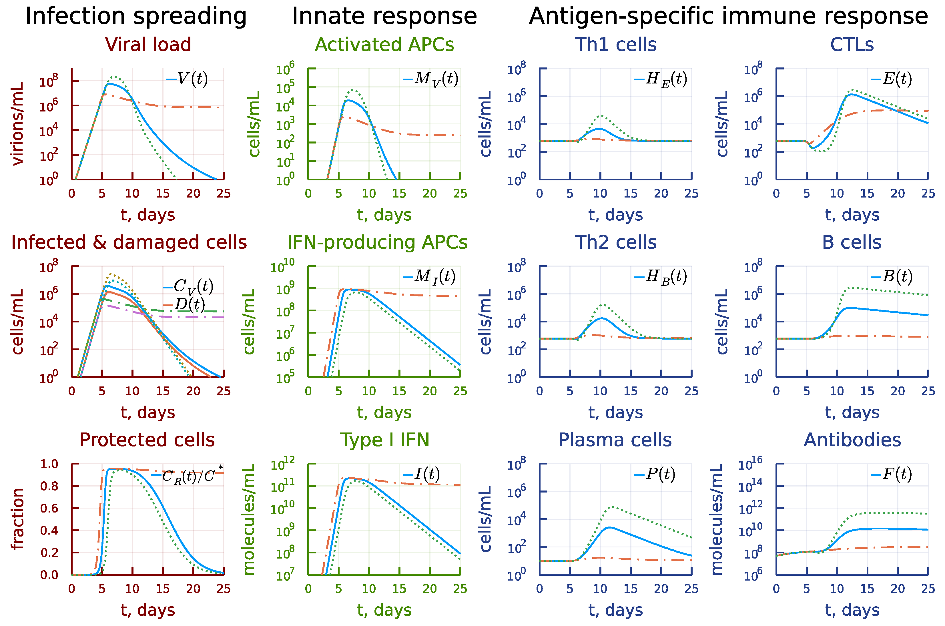
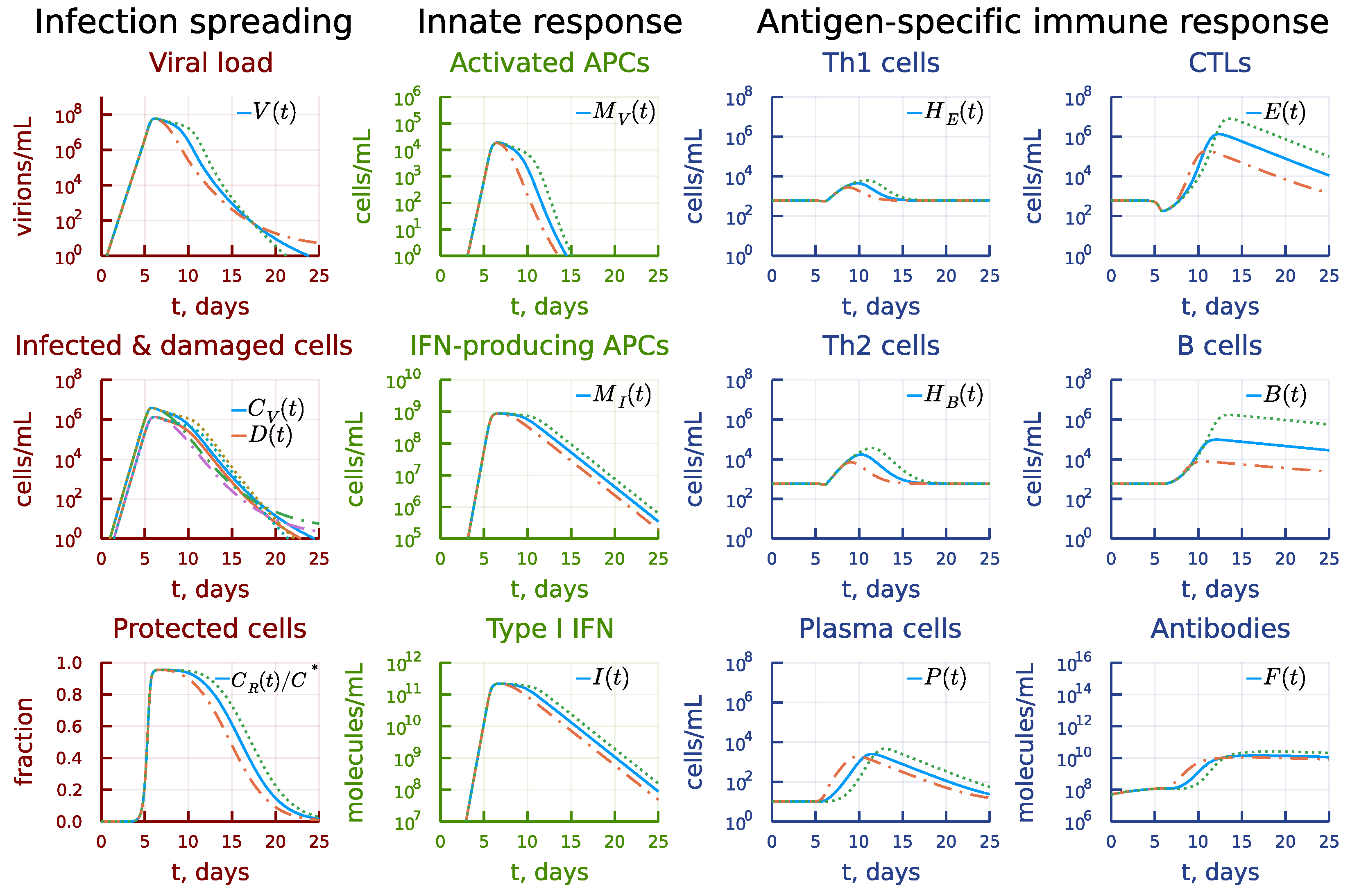
to examine the effect of the accelerated or decelerated components of the immune response on the viral load and prolonged viral persistence;

5.

to evaluate the person’s infectiousness and effectiveness of testing procedures.

To proceed with the analysis of SARS-CoV-2 infection, we consider our previously developed mathematical model of antiviral immune responses [23]. Recently, it was used to infer multiplicative cooperativity of CTL and antibody responses in protection against cytopathic and non-cytopathic virus infections [24]. Originally, the model was calibrated to describe an influenza A virus infection. Both influenza A and SARS-CoV-2 are controlled by immune reactions that proceed in the system of lymph nodes draining the upper and lower respiratory tract and follow a stereotypical clonal expansion kinetics. The use of the influenza infection model as a starting point to proceed with modelling of SARS-CoV-2 infection has been shown to be useful as providing some initial parameter values [3,8,17]. Using recently published extensive data sets on the kinetics of viral load in adult humans [25] as well as some other reference data for the observed levels of CD8 T cells, antibodies and type I IFNs in serum, we refine a subset of the model parameters to reproduce the observed dynamics of the SARS-CoV-2 loads. Then, the sensitivity of the infection characteristics to model parameters is computationally studied.

In Section 2 we present the details of the mathematical model, the data used for calibration and the resulting trajectory of SARS-CoV-2 infection in terms of model characteristics. Section 3 summarizes the results of computational experiments studying the effects of variations of the process parameters on kinetics of the viral load. Finally, in Section 4 we discuss the implications of our analysis for SARS-CoV-2 infection (long COVID) and the coordinated regulation of immune response components.

2. Materials and Methods

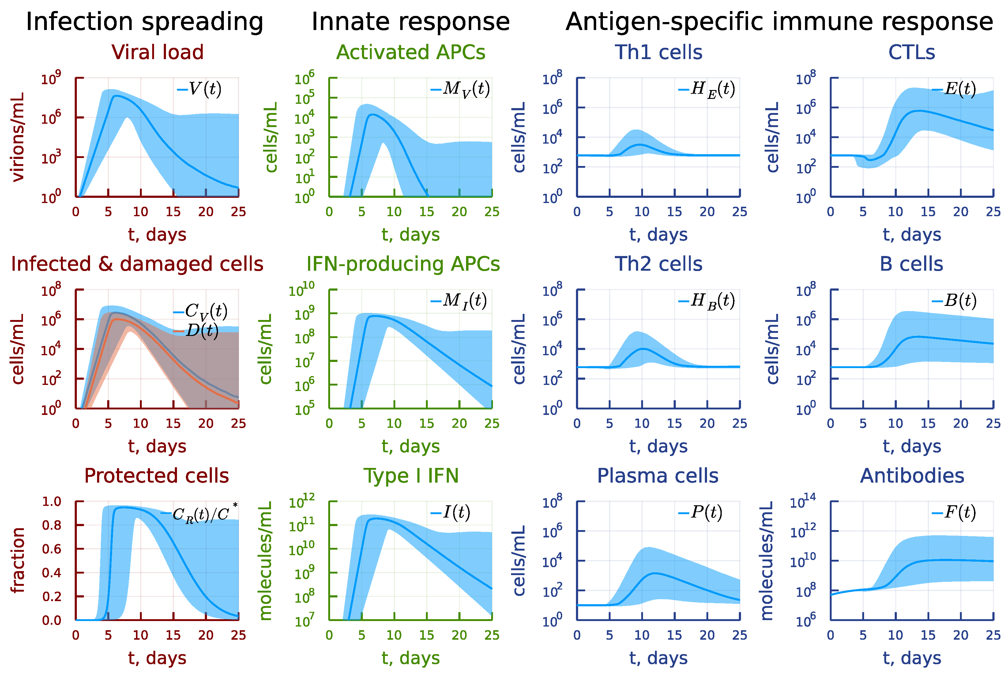
2.1. Mathematical Model of Antiviral Immune Response

Mathematical model of antiviral immune response considers three major sets of the virus-host interaction processes, i.e., the virus spreading in sensitive tissue, induction of the innate response and antigen-specific immune reactions as shown in Figure 1 and is described in details below. Consideration of innate cellular and humoral immune responses in conjunction with the infection of target organ cells and virus replication dynamics provides a tool to examine the joint impact and coordination of the considered arms of the immune system on the protection against virus infection and to reveal the critical aspects of developing disbalanced (biased) reactions.

2.1.1. Virus Spreading in Sensitive Tissue

SARS-CoV-2 targets primarily the respiratory tract spreading in upper (nasal mucosa and pharynx) and lower respiratory tract (bronchi and lungs). It infects epithelial cells, ciliated airway cells, alveoli Type 2 cells [26]. The rate of change of the populations of virus-infected target cells $C_V\left(t\right)$, type I interferon protected cells $C_R\left(t\right)$, damaged target cells $D\left(t\right)$, and freely circulating virus $V\left(t\right)$ is considered to be governed by the following equations:

$$\begin{array}{ccc}\hfill \frac{dV}{dt}\left(t\right)& =& \nu C_V\left(t\right)-({\gamma }_{VC}(C^{*}-C_V\left(t\right)-C_R\left(t\right)-D\left(t\right))+\hfill \\ & & {\gamma }_{VF}{f}_V\left(l\right)F\left(t\right)+{\gamma }_{VM})V\left(t\right),\hfill \end{array}$$

(1)

$$\begin{array}{ccc}\hfill \frac{d{C}_V}{dt}\left(t\right)& =& \sigma V\left(t\right)\left(C^{*}-C_V\left(t\right)-C_R\left(t\right)-D\left(t\right)\right)-(b_{CE}{f}_C\left(l\right)E\left(t\right)+b_m)C_V\left(t\right),\hfill \end{array}$$

(2)

$$\begin{array}{ccc}\hfill \frac{d{C}_R}{dt}\left(t\right)& =& {\sigma }_{R}I\left(t\right)\left(C^{*}-C_V\left(t\right)-C_R\left(t\right)-D\left(t\right)\right)-{\alpha }_R{C}_R\left(t\right),\hfill \end{array}$$

(3)

$$\begin{array}{ccc}\hfill \frac{dD}{dt}\left(t\right)& =& (b_{CE}{f}_C\left(l\right)E\left(t\right)+b_m)C_V\left(t\right)-{\alpha }_{m}D\left(t\right).\hfill \end{array}$$

(4)

2.1.2. Innate Immune Defence Reaction

The first line of reaction is related to sensing of the pathogen by the cells of the innate immune system. The innate immune response module considers the activation of professional antigen-presenting cells (including CD169 macrophages, and conventional dendritic cells, DCs) $M_V\left(t\right)$, type I Interferon (IFN) producing cells (including plasmacytoid DCs) $M_I\left(t\right)$, and type I IFN $I\left(t\right)$. The rate of changes of the concentration of these components is described by the following set of equations:

$$\begin{array}{ccc}\hfill \frac{d{M}_V}{dt}\left(t\right)& =& {\gamma }_{MV}{M}^{*}V\left(t\right)-{\alpha }_M{M}_V\left(t\right),\hfill \end{array}$$

(5)

$$\begin{array}{ccc}\hfill \frac{d{M}_I}{dt}\left(t\right)& =& {\gamma }_{M_I}(M_I^{*}-M_I)V\left(t\right)-{\alpha }_{M_I}{M}_I\left(t\right),\hfill \end{array}$$

(6)

$$\begin{array}{ccc}\hfill \frac{dI}{dt}\left(t\right)& =& {\rho }_I{M}_I\left(t\right)-({\sigma }_I(C^{*}-C_V\left(t\right)-C_R\left(t\right)-D\left(t\right))+{\alpha }_I)I\left(t\right).\hfill \end{array}$$

(7)

2.1.3. Antigen-Specific Immune Response

The viral antigens processed by antigen-presenting cells activate the clones of CD4 T cells (Th1 $H_E\left(t\right)$, Th2 $H_B\left(t\right)$), CD8 T cells $E\left(t\right)$, B cells $B\left(t\right)$, the latter resulting in the generation of plasma cells $P\left(t\right)$ and antigen-specific antibodies $F\left(t\right)$ via multiple interactions as shown in Figure 1. The respective equations of their dynamics have the structure presented below:

$$\begin{array}{ccc}\hfill \frac{d{H}_E}{dt}\left(t\right)& =& b_H^E(\xi \left(m\right){\rho }_H^E{M}_V(t-{\tau }_H^E)H_E(t-{\tau }_H^E)-M_V\left(t\right)H_E\left(t\right))\hfill \\ & & -b_p^{H_E}{M}_V\left(t\right)H_E\left(t\right)E\left(t\right)+{\alpha }_H^E(H_E^{*}-H_E\left(t\right)),\hfill \end{array}$$

(8)

$$\begin{array}{ccc}\hfill \frac{d{H}_B}{dt}\left(t\right)& =& b_H^B(\xi \left(m\right){\rho }_H^B{M}_V(t-{\tau }_H^B)H_B(t-{\tau }_H^B)-M_V\left(t\right)H_B\left(t\right))\hfill \\ & & -b_p^{H_B}{M}_V\left(t\right)H_B\left(t\right)B\left(t\right)+{\alpha }_H^B(H_B^{*}-H_B\left(t\right)),\hfill \end{array}$$

(9)

$$\begin{array}{ccc}\hfill \frac{dE}{dt}\left(t\right)& =& b_p^E(\xi \left(m\right){\rho }_E{M}_V(t-{\tau }_E)H_E(t-{\tau }_E)E(t-{\tau }_E)-M_V\left(t\right)H_E\left(t\right)E\left(t\right))\hfill \\ & & -b_{EC}{C}_V\left(t\right)E\left(t\right)+{\alpha }_E(E^{*}-E\left(t\right)),\hfill \end{array}$$

(10)

$$\begin{array}{ccc}\hfill \frac{dB}{dt}\left(t\right)& =& b_p^B(\xi \left(m\right){\rho }_B{M}_V(t-{\tau }_B)H_B(t-{\tau }_B)B(t-{\tau }_B)-M_V\left(t\right)H_B\left(t\right)B\left(t\right))\hfill \\ & & +{\alpha }_B(B^{*}-B\left(t\right)),\hfill \end{array}$$

(11)

$$\begin{array}{ccc}\hfill \frac{dP}{dt}\left(t\right)& =& b_p^P(\xi \left(m\right){\rho }_P{M}_V(t-{\tau }_P)H_B(t-{\tau }_P)B(t-{\tau }_P)+{\alpha }_P(P^{*}-P\left(t\right)),\hfill \end{array}$$

(12)

$$\begin{array}{ccc}\hfill \frac{dF}{dt}\left(t\right)& =& {\rho }_{F}P\left(t\right)-({\gamma }_{FV}V\left(t\right)+{\alpha }_F)F\left(t\right).\hfill \end{array}$$

(13)

2.1.4. Effects of Inflammation and Tissue Damage

Acute infection with SARS-CoV-2 is characterized by inflammatory reactions and immune cell recruitment to the site of infection [27]. To represent this enhancing effect of elimination on the infected cells and free viruses, the following parameterizations are used

$$\begin{array}{c}\hfill f_i\left(l\right)=1+{\mu }_{i}l,i=V,C,l=C_V\left(t\right)/C^{*}.\end{array}$$

(14)

Finally, severe damage of the upper and lower respiratory tract suppresses the antigen-specific immune responses [28,29]. This negative feedback regulation is taken into account via the following function

$$\begin{array}{c}\hfill \xi \left(D\right)=1-D\left(t\right)/C^{*}.\end{array}$$

(15)

2.1.5. Initial Conditions

The initial conditions for model Equations (1)–(15) were defined as folows:

$$\begin{array}{cc}\hfill & V\left(0\right)=V_0,H_E\left(0\right)=H_E^{*},H_B\left(0\right)=H_B^{*},E\left(0\right)=E^{*},\hfill \\ \hfill & B\left(0\right)=B^{*},P\left(0\right)=P^{*},F\left(0\right)=F^{*},\hfill \\ \hfill & C_V\left(0\right)=0,C_R\left(0\right)=0,D\left(0\right)=0,M_V\left(0\right)=0,M_I\left(0\right)=0,I\left(0\right)=0,\hfill \end{array}$$

(16)

where $V_0$ is the initial viral load in the upper respiratory tract, $H_E^{*}$, $H_B^{*}$, $E^{*}$ and $B^{*}$ are homeostatic concentrations for antigen-specific Th1, Th2, CTL and B cells in the lung-draining LNs, $P^{*}$ and $F^{*}$ are homeostatic concentrations for antigen-specific plasma cells and antibodies in blood, respectively. We assume no immune activation is present before the moment of infection:

$$M_V\left(t\right)=0,H_E\left(t\right)=H_E^{*},H_B\left(t\right)=H_B^{*},E\left(t\right)=E^{*},B\left(t\right)=B^{*},t<0.$$

(17)

2.2. Reference Data on SARS-CoV-2 Infection

In our study, we used recent data on viral kinetics during SARS-CoV-2 human challenge in young adults [25]. Healthy adult volunteers without evidence of previous infection were challenged intranasally with 10 TCID₅₀ of a wild-type SARS-CoV-2. Viral load in twice-daily nose and throat swab samples was measured by qPCR. The original data from 18 infected individuals were expressed as mean ± sem copies per mL. The data set on viral load kinetics to be used for model calibration was obtained using WebDigitizer from the Figure 2a of the published study. Mild-to-moderate symptoms defining the reference disease phenotype were observed in most (89%) of the participants starting from 2 to 4 days after inoculation. We did not consider the individual participant data as the summary statistics on the viral load consistently represent the infection kinetics of the above disease phenotype. The inter-patient variability of the viral load data is presented as pink shaded area in Figure 2. Additionally, the data on the scale of the interferon response [30], and the serum levels of the infected patients of antigen-specific antibodies and CTLs [31] were taken into account during the model calibration. The data ranges from the above studies are plotted as green shaded areas in Figure 2.

2.3. Calibration of the Model

The estimate for initial viral load $V_0$ can be derived from the experimental data on viral load [25] which we aim to reproduce. The participants were inoculated intranasally with the dose of 10 TCID₅₀ ≈ 7 PFU of SARS-CoV-2. To obtain the initial concentration $V_0$, we estimate the volume of nasal mucosa as 120–150 cm² of surface area times the thickness of 0.3–5 mm [32,33]. This gives us the range of values from 3.6 to 75 mL, with 7 mL being a harmonic mean. Thus, we fix $V_0\approx 7$ PFU/7 mL = 1 virion/mL. Note that more thorough estimates for infection dose and model parameters affecting the incubation period dynamics should be obtained using discrete-state stochastic models.

The homeostatic concentrations $H_E^{*}$, $H_B^{*}$, $E^{*}$, $B^{*}$ are estimated as follows: the frequency of antigen-specific cells is about ${10}^{-7}$–${10}^{-4}$ [34,35,36,37], there are about $2\times {10}^{11}$ immune cells of each type totally in approximately 1 litre of lymphoid tissue of the organism [38], the volume of the lung-draining lymphoid tissue is about 10 mL (=1%) [23], which gives the range $({10}^{-7},{10}^{-4})\times 2\times {10}^{11}\times 0.01/10=(20,\mathrm{20,000})$ cells/mL. We use the geometric mean of around 600 cells/mL for the point estimate. The estimates for $P^{*}$ and $F^{*}$ are borrowed from [23].

The calibration procedure consists of three stages: (i) deriving the estimates for admissible ranges and initial guesses of model parameters based on available literature, (ii) choosing a subset of parameters having a large effect on discrepancy between model solution and data based on sensitivity analysis, (iii) tuning parameters from a chosen subset in specified ranges to obtain an overall good fit, (iv) final refinement of parameters by solving a local nonlinear optimization problem to minimize the specified discrepancy.

The measure of discrepancy to be minimized is defined as

$$\mathsf{\Phi }\left(p\right)=\sum _{j=1}^M\left[{\left(\frac{V(t_j,p)-V_j^{obs}}{V_j^{obs}}\right)}^2+{\left(\frac{V(t_j,p)-V_j^{obs}}{V(t_j,p)}\right)}^2\right],$$

(18)

where $V(t_j,p)$ is the viral load predicted by the model with parameter values p at M time points $t_j$, $V_j^{obs}$ is the experimental data on viral load at corresponding time points. This functional weighs similarly both deviations at high and low viral load values [23].

As a starting point, we used the parameter values and ranges specified in the previously calibrated model of influenza A virus infection [23,24]. Some parameter estimates were refined, as described below.

To determine a subset of parameters to variate, we analyzed the sensitivity of parameters towards the partial sums of functional (18) at certain time points, corresponding to different stages of infection (see Section 2.4). We can select the following parameters as having the most effect on each stage:

• First stage (incubation period, 0–3 days): $\nu ,\sigma ,{\gamma }_{VC},{\gamma }_{VM}$.
• Second stage (activation of immune response and peak of viral load, 4–7 days) and third stage (recovery period, 8–13 days): ${\sigma }_R,{\rho }_I,{\gamma }_{VF},{\gamma }_{FV},{\sigma }_I,{\mu }_V,{\gamma }_{M_I},b_p^P,{\gamma }_{MV}$.
• Forth stage (post-symptomatic period, 14–19 days): $b_{CE},{\gamma }_{VC},b_H^B$.

Note that some parameters naturally have influence on several stages. However, one can derive a good fit by sequentially tuning the subsets of parameters for each stage. Also, the parameters reported above don’t include parameters for which we already have a good estimate and narrow ranges from [23].

For the rate of SARS-CoV-2 virions secretion per infected epithelial cell, $\nu$, we set the initial guess $\nu =130$ day⁻¹ and admissible range $(10,1000)$ day⁻¹ based on our previous experience of modelling SARS-CoV-2 replication cycle [39,40].

The infection rate of target epithelial cells with SARS-CoV-2, $\sigma$, can be estimated as $\sigma \approx 1/(t_{l.c.}\times V_{MOI}\times f_D\times C^{*})$, where $t_{l.c.}$ is a typical duration of the intracellular replication cycle, $V_{MOI}$ is a multiplicity of single cell infection, and $f_D$ is a fraction of epithelial cells in lungs damaged during infection [23]. Taking the ranges $t_{l.c.}\in (7,24)$ h, $V_{MOI}\in (1,10)$ [39,40], and $f_D\in (0.1,0.5)$, $C^{*}\in ({10}^9,{10}^{10})$ cells [23], we arrive to the estimate $\sigma \in (2\times {10}^{-11},3\times {10}^{-8})$ (cells/mL)⁻¹day⁻¹.

The expenditure rate of virions on the infection of target cells, ${\gamma }_{VC}$, should be balanced with the infection rate $\sigma$. These parameters can be related through ${\gamma }_{VC}=V_{MOI}\times \sigma$, where $V_{MOI}$ is the number of virions infecting a single target cell, for which we set the initial guess and the range $V_{MOI}=10\in (1,20)$.

The rate of CTL-mediated destruction of epithelial cells, $b_{CE}$, can be estimated using the scheme suggested in [23]: $b_{CE}\approx 1/(t_{LN\to RT}\times E_{suf})$. Here, $E_{suf}$ is the number of CTLs sufficient to destroy $f_D\times C^{*}$ epithelial cells, and $t_{LN\to RT}\in (2,12)$ h is the typical time for a CTL to reach the target compartment of respiratory tract mucosa from LNs draining the lungs. As one CTL can destroy several target cells (≈10), the estimate is $b_{CE}\in (4\times {10}^{-9},4\times {10}^{-7})$ (virions/mL)⁻¹day⁻¹.

We used the estimates as initial guesses and ranges from [23] for parameters ${\gamma }_{VM},{\gamma }_{M_I}$, ${\sigma }_R,{\sigma }_I,{\gamma }_{VF},{\gamma }_{FV},{\mu }_V,b_p^P,b_H^B$.

The remaining model parameters were not varied; instead, their values were fixed to the estimates from [23]. Note that concentrations are reported in

Table 1. Parameters of the calibrated model.

	Parameter, Units	Range, Initial Guess	Estimate
$M^{*}$	Concentration of APCs, cells/mL	$(3\times {10}^5,2\times {10}^6)$	$6\times {10}^5$
$M_I^{*}$	Concentration of IFN-producing APCs, cells/mL	$({10}^7,{10}^9)$	${10}^9$
$H_E^{*}$	Concentration of SARS-CoV-2 specific Th1 cells, cells/mL	$(20,20,000)$	600
$H_B^{*}$	Concentration of SARS-CoV-2 specific Th2 cells, cells/mL	$(20,20,000)$	600
$E^{*}$	Concentration of SARS-CoV-2 specific CTLs, cells/mL	$(20,20,000)$	600
$B^{*}$	Concentration of SARS-CoV-2 specific B cells, cells/mL	$(20,20,000)$	600
$P^{*}$	Concentration of SARS-CoV-2 specific plasma cells, cells/mL	$(2,42)$	10
$F^{*}$	Concentration of SARS-CoV-2 specific antibodies, molecules/mL	$({10}^7,{10}^8)$	$5\times {10}^7$
$C^{*}$	Concentration of epithelial cells, cells/mL	$({10}^9,{10}^{10})$	${10}^{10}$
${\alpha }_M$	Rate of stimulated state loss for APCs, day−1	$(1,3.3)$	$3.3$
${\alpha }_H^E$	Rate of activated state loss for Th1 cells, day−1	$(0.8,1.2)$	1
${\alpha }_H^B$	Rate of activated state loss for Th2 cells, day−1	$(0.8,1.2)$	1
${\alpha }_E$	Rate of natural death for CTLs, day−1	$(0.33,0.5)$	$0.4$
${\alpha }_B$	Rate of natural death for B cells, day−1	$(0.05,0.1)$	$0.1$
${\alpha }_P$	Rate of natural death for plasma cells, day−1	$(0.33,0.5)$	$0.4$
${\alpha }_F$	Rate of natural death for antibodies, day−1	$(0.033,0.1)$	$0.043$
${\tau }_H^E$	Duration of Th1 cell division cycle, days	$(0.4,0.8)$	$0.6$
${\tau }_H^B$	Duration of Th2 cell division cycle, days	$(0.4,0.8)$	$0.6$
${\tau }_E$	Duration of CTL division cycle, days	$(0.5,1)$	$0.5$
${\tau }_B$	Duration of B cell division cycle, days	$(0.5,1)$	$0.5$
${\tau }_P$	Duration of B cell differentiation into plasma cells, days	$(0.5,1)$	$0.5$
${\rho }_H^E$	Number of Th1 cells created during division cycle	$(2,4)$	4
${\rho }_H^B$	Number of Th2 cells created during division cycle	$(2,4)$	4
${\rho }_E$	Number of CTLs created during division cycle	$(2,4)$	2
${\rho }_B$	Number of B cells in clone created by series of 1 or 2 divisions	$(1.5,3)$	3
${\rho }_P$	Number of plasma cells in clone created by series of 1 or 2 divisions	$(0.5,1)$	1
${\rho }_F$	Rate of IgG production per plasma cell, molecules/cell/day	$(8.5\times {10}^5,1.7\times {10}^6)$	$1.7\times {10}^6$
$b_H^E$	Rate of Th1 cells stimulation, (cells/mL)−1day−1	$(5\times {10}^{-7},4.5\times {10}^{-4})$, $4.5\times {10}^{-5}$	$4.8\times {10}^{-5}$
$b_H^B$	Rate of Th2 cells stimulation, (cells/mL)−1day−1	$(5\times {10}^{-7},4.5\times {10}^{-4})$, $4.5\times {10}^{-5}$	$9.2\times {10}^{-5}$
$b_p^E$	Rate of CTL stimulation, (cells/mL)−2day−1	$(6\times {10}^{-11},4\times {10}^{-6})$, $1.4\times {10}^{-8}$	$2.4\times {10}^{-6}$
$b_p^B$	Rate of B cell stimulation, (cells/mL)−2day−1	$(6\times {10}^{-12},5\times {10}^{-8})$, $2.2\times {10}^{-9}$	$3.9\times {10}^{-8}$
$b_p^P$	Rate of plasma cell stimulation, (cells/mL)−2day−1	$(1.4\times {10}^{-10},3\times {10}^{-9})$, $2.2\times {10}^{-9}$	$3\times {10}^{-9}$
$b_p^{H_E}$	Rate of Th1 cells suppression, (cells/mL)−2day−1	$(6\times {10}^{-15},4\times {10}^{-10})$	$2.8\times {10}^{-13}$
$b_p^{H_B}$	Rate of Th2 cells suppression, (cells/mL)−2day−1	$(6\times {10}^{-16},5\times {10}^{-12})$	$2.8\times {10}^{-13}$
${\gamma }_{MV}$	Rate of APC stimulation, (cells/mL)−1day−1	$(1.7\times {10}^{-13},{10}^{-7})$, $2\times {10}^{-6}$	$1.9\times {10}^{-9}$
${\gamma }_{FV}$	Rate of IgG binding to SARS-CoV-2, (virions/mL)−1day−1	$(1.4\times {10}^{-10},1.4\times {10}^{-8})$, $1.4\times {10}^{-9}$	$2.8\times {10}^{-9}$
$\sigma$	Rate of epithelial cell infection with SARS-CoV-2, (cells/mL)−1day−1	$(2\times {10}^{-11},3\times {10}^{-8})$, ${10}^{-10}$	$1.4\times {10}^{-10}$
$b_{CE}$	Rate of infected epithelial cell damage by CTLs, (virions/mL)−1day−1	$(4\times {10}^{-9},4\times {10}^{-7})$, $5\times {10}^{-8}$	$4\times {10}^{-9}$
$b_{EC}$	Rate of CTL death due to lytic interactions with infected cells, (cells/mL)−1day−1	$({10}^{-10},4\times {10}^{-7})$	$2.7\times {10}^{-10}$
$b_m$	Rate of infected cell damage due to SARS-CoV-2 cytopathicity, day−1	$(0.5,2)$	$1.5$
${\alpha }_m$	Rate of epithelial cell regeneration, day−1	$(1,4)$	4
$\nu$	Rate of SARS-CoV-2 virions secretion per infected epithelial cell, day−1	$(10,{10}^4)$, 130	144
${\gamma }_{VC}$	Rate of SARS-CoV-2 absorption by epithelial cell, (cells/mL)−1day−1	$(2\times {10}^{-11},6\times {10}^{-7})$, ${10}^{-9}$	$3.2\times {10}^{-9}$
${\gamma }_{VM}$	Rate of nonspecific SARS-CoV-2 elimination, day−1	$(2,4)$, $1.7$	4
${\gamma }_{VF}$	Rate of SARS-CoV-2 neutralization by specific IgG, (virions/mL)−1day−1	$(1.4\times {10}^{-11},1.4\times {10}^{-8})$, $1.4\times {10}^{-9}$	$1.4\times {10}^{-8}$
${\mu }_V$	Parameter for inflammation-based enhancement of IgG effect	$(10,{10}^5)$, 1000	2628
${\mu }_C$	Parameter for inflammation-based enhancement of CTL effect	$(10,{10}^5)$, 1000	1407
${\gamma }_{M_I}$	Rate of induction of IFN-producing state in APCs, (cells/mL)−1day−1	$(2.3\times {10}^{-9},2.3\times {10}^{-7})$, $1.7\times {10}^{-8}$	$5.7\times {10}^{-8}$
${\alpha }_{M_I}$	Rate of IFN-producing state loss by APCs, day−1	$(0.3,0.5)$	$0.5$
${\rho }_I$	Rate of IFN production per IFN-producing cells, molecules/cell/day	$(500,12,000)$	6000
${\alpha }_I$	Type I IFN clearance rate, day−1	$(10,100)$	24
${\sigma }_I$	Rate of IFN binding with epithelial cells, (cells/mL)−1day−1	$(1.7\times {10}^{-11},1.7\times {10}^{-9})$, $1.7\times {10}^{-9}$	$1.7\times {10}^{-11}$
${\sigma }_R$	Rate of virus-resistant state induction in epithelial cells, (cells/mL)−1day−1	$(3.3\times {10}^{-12},3.3\times {10}^{-10})$, $3.3\times {10}^{-11}$	$9.9\times {10}^{-11}$
${\alpha }_R$	Rate of virus-resistant state loss in epithelial cells, day−1	$(0.5,1.5)$	1

as numbers of cells, virions or molecules per mL as opposed to molar units used in the previous work.

For final stage of calibration, we numerically solved a problem of minimizing (18) with respect to parameters, using a local method. We used first the derivative-free Nelder-Mead method, followed by the derivative-based quasi-Newton L-BGFS method using the meta-package Optimization.jl in julia language.

The final estimates of calibrated model parameters p are presented in Table 1. Initial guess is reported only for parameters which were tuned during the calibration process. The calibrated model parameters correspond to discrepancy $\mathsf{\Phi }\left(p\right)=1086$. The baseline solution of the model describing the intra-host SARS-CoV-2 infection and antiviral immune response dynamics and the available clinical data are shown in Figure 2.

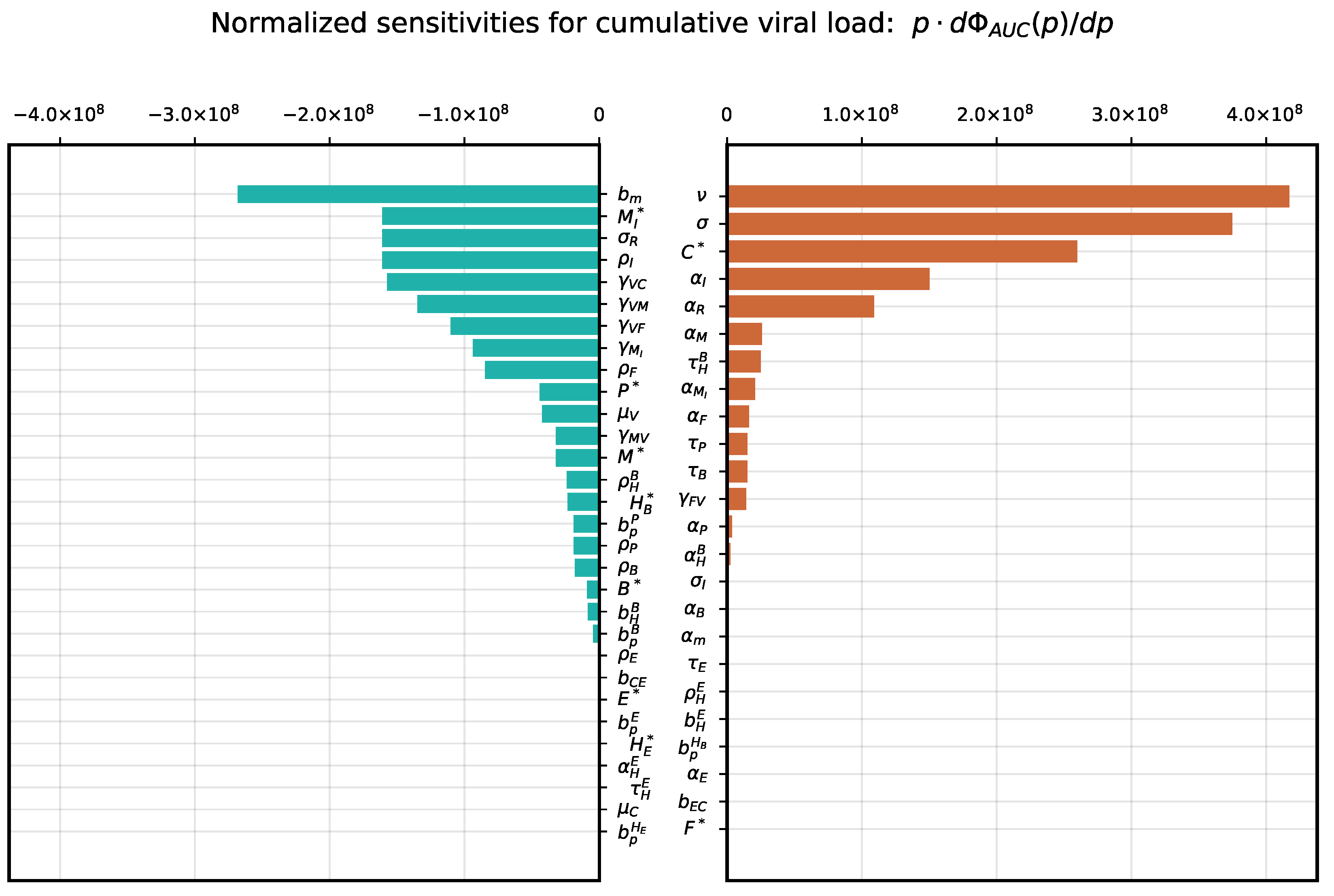
2.4. Sensitivity Analysis

Sensitivity analysis was employed both as exploratory tool in the calibration process, and as a way to derive meaningful predictions of the calibrated model. We used a local sensitivity approach, in which sensitivity indices of some functional of the model solution $\mathsf{\Phi }\left(y\right(p\left)\right)$ with respect to variations in model parameters $p_j$ are defined as

$$s_j=\frac{d\mathsf{\Phi }}{d{p}_j}\left(p\right),{\widehat{s}}_j=p_j{s}_j,$$

(19)

and provide a measure of the influence of parameter variations on the functional. The normalized version ${\widehat{s}}_j$ of sensitivity indices provides the way to compare and rank the parameters based on their effect.

We used the following functionals of interest in this work:

$${\mathsf{\Phi }}_{AUC}={\int }_0^{T}V\left(t\right)dt,{\mathsf{\Phi }}_{peak}=\underset{t\in [0,T]}{max}\left(V\left(t\right)\right),$$

(20)

where ${\mathsf{\Phi }}_{AUC}$ refers to the cumulative viral load during the time course of infection, ${\mathsf{\Phi }}_{peak}$ is the peak viral load. Additionally, we analyzed sensitivity of the functional of discrepancy with experimental data (18) at various subsets of time points during the calibration process. The value of T is taken to be 25 days corresponding to the time of virus clearance according to the clinical data. All sensitivity indices were calculated using forward-mode automatic differentiation available in the package ForwardDiff.jl in julia language.

The calibrated mathematical model is a nonlinear system of equations with parameters characterized by uncertainty ranges specified in Table 1. Hence, a global sensitivity analysis of the model output is required to complement the local analysis. A likely non-monotonic relationship between the parameters and the model output suggests that the variance-based method of sensitivity analysis based on decomposition of the output variance needs to be applied. We utilized the extended Fourier Amplitude Sensitivity Test (eFAST) method which allows to quantify the fraction of the model output variance that can be explained by variation in every model input parameter [42]. The total number of samples per search curve was $N_s=2000$. The eFAST provides the estimates of the first-order sensitivity and total-order sensitivity for each model parameter. They were averaged over $N_r=10$ resamples.

3. Results

3.1. Local Sensitivity Analysis

The sensitivity analysis of the cumulative viral load, which is an important characteristic affecting positively and negatively the dynamics of immune responses [43], showed a strong positive dependence on the virus secretion rate, the target cell infection rate and the number of available target cells expressing ACE2. It is most strongly negatively affected by the parameter of innate immune response related to activation of APCs and type I IFN system as summarized in Figure 3. The peak viral load has a similar sensitivity ranking with respect to the most influential parameters, see Figure 4.

3.2. Global Sensitivity Analysis

To examine the variability of the model output emerging from uncertainty in parameter values, a global sensitivity analysis was performed by applying the eFAST method. As model solution-dependent functional, we considered two model outputs, i.e., cumulative viral load and the peak viral load. Although the estimates for the admissible ranges on model parameters are specified in Table 1, a direct use of them as lower and upper bounds in sampling parameters might be inappropriate as these ranges characterize the uncertainty for each individual parameter without taking into account their possible interactions. To keep the parameter uncertainty within the range consistent with the mild-to-moderate disease phenotype, the respective scale of the parameter variance was identified to be around 20% of the basal values. The 90% band characterising the variability of the model solution is shown in Figure 5. The uniform distribution on the ranges was assumed for all model parameters. The results are summarized in Figure 6 and Figure 7, respectively. For both outputs, the virus spreading parameters in target organs, the free virus elimination rates and the type I IFN response demonstrate the strongest parameter-specific contribution to the variability in virus dynamics.

3.3. Induction of Antigen-Presenting Cells

The cascade of antiviral immune responses starts with activation of antigen-presenting cells. The sensitivity threshold is characterized by the model parameter ${\gamma }_{MV}$. We examined the effect of its 10-times increase and decrease on the course of the virus infection as shown in Figure 8 characterizing the rate constant of the antigen-presenting cell stimulation. The model predicts that a higher sensitivity induces faster and stronger responses, which spread through the whole response cascade (see the panel under heading Antigen-specific immune response). However, a ten-fold decrease results in higher viral antigen levels which are needed to induce activation of the immune system, which delays the immune response and finally favours prolonged viral persistence (see the panel under heading Infection spreading). Interestingly, that a stronger type I IFN response is not sufficient to clear the infection in this case (see the panel under heading Innate response).

3.4. Induction of Type I IFN Response

The ten-fold increase in the rate constant of activation of type I IFN response ${\gamma }_{M_I}$ results in a lower viral peak, as one can see in Figure 9 (see also the panel under heading Infection spreading). However, this affects the activation of antigen-presenting cells and the resulting reduced response percolates through to antigen-specific arms (see the panel under heading Innate response). Both the T-cell and B-cell responses appear to be weaker (see the panel under heading Antigen-specific immune response). The virus is not eliminated within 25 days, so that the viral persistence is observed. A similar decrease in ${\gamma }_{M_I}$ leads to a poorer control of viral load so that it reaches higher peaks. The antigen-specific response turns out to be stronger. However, the damage of the target organs also increases by one order of magnitude.

The effect of 10-fold variation of the parameter ${\sigma }_R$ characterizing the rate constant of type I IFN-mediated induction of resistance to infection of target cells expressing ACE2 is displayed in Figure 10. Its impact on the solution of the model is similar to that of ${\gamma }_{M_I}$.

3.5. Disregulation of CTL and B-Cell Responses

Next, we examined the extent of kinetic cooperativity between the T- and B cell responses. To this end, a 10-fold variation was applied to parameter $b_p^B$, the clonal activation rate constant of B cells. The results are summarized in Figure 11. An earlier activation of the humoral immune response (see the panel under heading Antigen-specific immune response) results in faster (by 5 days) viral elimination (see the panel under heading Infection spreading) but reduces the CTL response (see the panel under heading Antigen-specific immune response). A delayed activation of B cells critically affects the dynamics of infection, resulting in a prolonged viral persistence.

A similar exploration of the effect of two-fold increasing the activation rate constant of CTL clonal expansion, i.e., $b_p^E$, at the background of an opposite two-fold variation of the activation rate of B cells $b_p^B$ is shown in Figure 12. The increase in CTL responsiveness turns out to be much stronger (see the panel under heading Antigen-specific immune response) but it fails to eliminate the infection (see the panel under heading Infection spreading) because the humoral immune response is not sufficient. The effect of the reduced activation rate of CTL response can be compensated by a two-fold increase in the activation rate of B cells, so that the infection is completely eliminated.

The 10-fold increase in the differentiation rate constant of antigen-specific B cells into plasma cells $b_p^P$ leads to an earlier appearance of antibodies, as displayed in Figure 13 (see the panel under heading Antigen-specific immune response). However, the clonal expansion of B cells and CTL is smaller, which finally results in failure of the system to eliminate the virus (see the panel under heading Infection spreading). Reduced differentiation rate slightly increases the duration of the peak viral load but stronger B- and T cell responses finally eliminate the virus infection five days earlier compared to the basal solution pattern.

A higher extent of variation of the differentiation rate of B cells into plasma cells $b_p^P$ (i.e., by 40-times) changes the dynamics as shown in Figure 14. The respective increase results in sufficient production of antibodies (see the panel under heading Antigen-specific immune response) eliminating the virus (see the panel under heading Infection spreading). However, the cumulative viral load is smaller and, hence, we observe the expansion of T cells and B cells. The decrease of the differentiation rate of B cells into plasma cells results in an delayed but enhanced Th1, Th2, CTL and B cell and plasma cell expansion (see the panel under heading Antigen-specific immune response). This solution trajectory is characterized by a higher number of damaged infected target cells and prolonged viral persistence at the peak levels (see the panel under heading Infection spreading).

3.6. Asymmetry of Th1 versus Th2 Responses

It has been recently observed that epidemiological data show a reduced risk of severe COVID-19 in SARS-CoV-2 infected patients with the type 2 asthma [44]. Asthma is considered to be associated with a dominance of T helper 2 (Th2) cells. We used the model to predict the impact of a stronger activation rate constant of Th2 cells $b_H^B$ compared to Th1 cells on the dynamics of infection. The results are presented in Figure 15. The ten-fold increase of the clonal expansion rate of Th2 cells leads to an earlier elimination of virus (see the panel under heading Infection spreading) due to enhanced (by several orders or magnitude) humoral immune response, with the CTL response left almost unchanged (see the panel under heading Antigen-specific immune response). However, a similar reduction in the activation rate essentially reduced all components of the B-cell and antibody responses. The stronger induction of CTL response is not enough to compensate for the weaker humoral immune response and the prolonged viral persistence is predicted.

The biased towards Th2 cells antigen-specific immune response could also be a consequence of a larger homeostatic number of this population compared to Th1 cells, i.e., the concentration of SARS-CoV-2 specific Th2 cells. Figure 16 shows the effect of a five-times variation of the respective parameter $H_B^{*}$. A higher initial number of SARS-CoV-2-specific Th2 cells leads to an earlier and stronger B-cell response (see the panel under heading Antigen-specific immune response) and faster virus elimination (see the panel under heading Infection spreading). Similar reduction results in a delayed CTL and B-cell responses and prolonged viral persistence.

3.7. Kinetic Mechanisms of Long COVID-19 Pathogenesis

Following the above examination of the degree of synchrony in the cascade of antiviral immune response, we estimated the degree of variation in the respective parameters which lead to prolonged viral persistence, i.e., beyond 30 days post infection. The results are summarized in

Table 2. Thresholds for individual parameter variations which lead to virus persistence. Abbreviations for the parameters: ${\gamma }_{MV}$—rate constant of APC stimulation; $b_p^P$—rate constant of plasma cell stimulation; $b_p^B$—rate constant of B cell stimulation; $b_p^E$—rate constant of CTL stimulation; $b_H^B$—rate constant of Th2 cells stimulation; $b_H^E$—rate constant of Th1 cells stimulation; ${\gamma }_{M_I}$—rate constant of induction of IFN-producing state in APCs; ${\sigma }_R$—rate constant of virus-resistant state induction in epithelial cells; ${\mu }_V$—parameter for accounting the inflammation-based enhancement of IgG effect; ${\mu }_C$—parameter for accounting the inflammation-based enhancement of CTL effect.

Parameter	${\gamma }_{MV}$	$b_p^P$	$b_p^B$	$b_p^E$	$b_H^B$	$b_H^E$	${\gamma }_{M_I}$	${\sigma }_R$	${\mu }_V$	${\mu }_C$
Variation	$÷1.12$	$\times 3$	$÷1.4$	−	$÷1.15$	−	$\times 1.15$	$\times 1.06$	$\times 1.3$	$\times 8\times {10}^4$

.

The model predicts that a 12%, 15% and 6% shift in the values of innate immune cell activation parameters, i.e., ${\gamma }_{MV}$, ${\gamma }_{M_I}$, ${\sigma }_R$ respectively, turns out to be sufficient to extend the viral persistence beyond 30 days post infection. Thus, the kinetic ratios between the parameters of the innate immunity (rate of APCs activation, rate of induction of IFN-producing state in APCs and rate of virus-resistant state induction in epithelial cells) appeared to be of high importance for the host to resist the infection and to eliminate the virus quickly. The model predicts that 12% decrease of activated APCs could result in a prolonged virus persistence and can be dangerous. Indeed, severe SARS-CoV-2 infection is associated with the impaired ability of dendritic cells to present antigens and to produce type-I IFN [45]. The robustness with respect to the B cell proliferation and differentiation shift is stronger. The inflammation-related enhancement of virus- and infected cell elimination parameters ${\mu }_V$, ${\mu }_C$ is robust to 30% and $8\times {10}^4$-fold increase, respectively. 15% reduction of the activation rate of Th2 cells compared to Th1 cells results in prolonged virus persistence.

3.8. Individual’s Infectiousness

The kinetics of the viral load in upper respiratory tract reproduced by the model can be translated into the estimates of the number of viruses expelled by an infected individual during talking via droplets [9]. Given the estimate of the volume of the expelled droplets $V_{droplets}=1.1\times {10}^{-4}$ mL [9], we can obtain the number of expelled virions (infectiousness) as $V_{droplets}\times V\left(t\right)$. The time-course of an airborne transmission intensity of an infected person as predicted by the calibrated model is presented in Figure 17.

3.9. Day-by-Day Use of the Model

Mathematical models provide a theoretical tool to describe, explain, and predict the features of SARS-CoV-2 interaction with the human organism. The developed model of infection with SARS-CoV-2 describes some of the available patients’ data [25]. It proposes a novel hypothesis on the effect of kinetic coordination of innate and adaptive immune reactions in the establishment of prolonged viral persistence. A rigorous validation of this conceptually new regulatory mechanism requires substantial well controlled experimental and clinical studies and thus goes beyond the scope of our research. To illustrate the power of the model in addressing existing controversial issues concerning the pathogenesis and treatment of SARS-CoV-2 infection, we added the analysis of the effect of passive immunotherapy with virus-specific antibodies on the duration of the infectiousness and symptoms for COVID-19 patents. The existing treatments with immunoglobulins include the use of convalescent plasma therapy, intravenous immunoglobulins, and monoclonal antibody therapy [46]. The regimens used are highly variable [47,48]. As a proof-of-concept, we simulated a daily introduction of virus-specific IgG at doses ranging from $0.4\times {10}^{10}$ to ${10}^{11}$ molecules/mL starting from day 2 post establishment of symptoms during 5 days treatment period. The model predicts that 25-times increase of the dose of administered IgG results in shortening of the period of viral load above the infectiousness threshold from 7 days to 3 days for the considered set of model parameters as shown in Figure 18. Further translation of the predicted dynamics of viral load into infectiousness of the patients requires application of the probabilistic model linking the viral load to the infectiousness, as elaborated recently in [21]. The duration of the symptomatic period of COVID-19 reduced from 8 to 3.6 days. The simulations also showed that smaller amounts (below some threshold) of IgG can favour a prolonged viral persistence resembling the experimental observation that convalescent plasma, administered to medium titers, has limited efficacy, even when given very early after infection [47]. Overall, these model-generated predictions corroborate empirical findings that the use of high doses of virus-specific immunolglobulins in treatment of COVID-19 is effective but not without potentially adverse consequences [47,49,50].

4. Discussion

In this study we developed a calibrated mathematical model of antiviral immune response to SARS-CoV-2 infection. Recently published data sets from the human challenge studies with SARS-CoV-2 were used for parameter estimation [25]. The viral load data for the model calibration characterize the kinetics in the upper respiratory tract (the nose compartment). The data on the scale of the interferon response [30], the antigen-specific antibodies and CTLs [31] refer to their respective levels in serum of the infected patients. The model considers innate and antigen-specific responses to SARS-CoV-2 infection. In turn, the innate subsystem of equations describes the dynamics of the type I IFN response and antigen presentation. The antigen specific immune response includes the clonal dynamics of Th1- and Th2 CD4 T cells, CD8 T cells, B cells, plasma cells and antibodies. The effect of inflammatory responses on elimination of the virus and infected cells is taken into account. The damage of the infected target cells (epithelial and endothelial cells, ciliated airway cells, alveoli type 2 cells) results in the suppression of antigen-specific immune responses. In our view, the model details provide an appropriate balance between the description of the complexity of SARS-CoV-2 infection and the consistency with the quantitative view of a mild-to-moderate symptoms COVID-19 [1,30,31,51].

Consideration of multiple immune reaction components in a single calibrated mathematical model allows one to address some fundamental issues related to the pathogenesis of COVID-19, e.g., sensitivity of peak viral load to parameters characterizing specific response components, the kinetic coordination of the individual responses, and factors favoring prolonged viral persistence. The sensitivity of the dynamics of viral load to the activation rates of the immune system components is examined at two scales, i.e., a fine-resolution scale and globally. The first one allowed us to identify the exact biases in the activation rates that lead to a prolonged persistence of SARS-CoV-2. To check whether this phenomenon is robust, we also considered a large-scale variation of the activation rates, e.g., the 10-fold change of the respective parameters.

Our model-based analyses suggest that the sequele of immune responses differentially mounted by innate and adaptive subsystems needs to be kinetically synchronized to ensure an optimal induction of the whole cascade. An improper increase in the activation rate of a single component may cause reduced responses of the others, thus favouring the virus persistence. This observation corroborates results of the recent studies on age-related differences in immune dynamics in SARS-CoV-2 infection of non-human primates [52] and a delayed viral clearance in some asymptomatic human infections [53]. It was summarized that the major difference between the young and old rhesus macaques is a much stronger innate response and a delayed antigen-specific response in older animals [52]. The dysregulation of innate and adaptive immune responses was considered to result in a prolonged SARS-CoV-2 persistence [53].

The above finding bears a direct implication for a mechanistic understanding of prolonged viral persistence, i.e., beyond 30 days post infection. The problem of long COVID-19 is emerging as a key pathological consequence of SARS-CoV-2 infection [54,55]. Although the set of etiological factors is very broad [56], the residual persistence of viral RNA is considered among them [57]. We identified the thresholds in the increase of the innate and adaptive responses parameters which lead to a prolonged persistence of SARS-CoV-2 due to the loss of a kinetic synchrony/coordination of the responses, i.e., to the loss of an optimal pattern of their cascade. We suggest that the parameters from Table 2 could appear useful for clinical physicians in predicting the disease outcome. Finally, the model can be used to predict the intensity of airborne infection spreading by infected individuals, e.g., the amount of virus which is transmitted via droplets from a SARS-CoV-2 infected person, depending on the time of infection and the immune response parameters. This type of estimates provide a direct information that may be included in the epidemiological models of virus spreading in the human population [58,59]. We note that a probabilistic model was recently elaborated linking the viral load and the host infectiousness [21]. It was used to evaluate the effectiveness of PCR and antigen-based testing.

Calibration of the developed model of SARS-CoV-2 infection is based on a limited set of empirical data. However, for all processes considered in the model, various parameterizations could be used. To proceed with the identification of optimal descriptions of the immune responses to SARS-CoV-2, quantitative definitions of COVID-19 dynamics- and outcome phenotypes are needed. These should define the regulation levels, processes, tissues and organs to be considered in the models and enable a rational implementation of the reductionist approach to model refinement. A final objective would be the application of the minimum description length-based methodology for a parsimonious mapping (using the model equations) of the virus and immune system parameters to the observed spectrum of COVID-19.

From an immunophysiological side, the future development of the model will be related to a fine tuning of parameters and compartmental (multi-organ) extension of the equations to deal with the systemic aspects of COVID-19 [27,60]. A fundamental issue which remains to be explored is the incorporation of the regulatory feedbacks into the model, e.g., taking into account the pleiotropic effects of type I IFN, cytokines and networking of immune cells subsets. However, these refinements should go in coordination with clinical and experimental studies so that the increase of the model complexity could be justified.

The calibration of the mathematical model of SARS-CoV-2 infection is based on combining the parameter guesses from our earlier study of influenza A virus infection, some recent quantitative models of SARS-CoV-2 infection and clinical data-based parameter estimation of a subset of the model parameters. Hence, the calibrated mathematical model represents a theoretical exploration type of study, i.e., ‘in silico patient’ with mild-to-moderate severity phenotype, rather than a completely validated quantitative model of COVID-19 regarding all its state-space variables.

The local sensitivity analysis allowed us to evaluate the effects of small parameter variations around the model parameters which were calibrated to describe the mild-to-moderate disease phenotype. For parameter sets corresponding to another clinical outcome, e.g., asymptomatic, severe or critical phenotype, the local sensitivity indices could change significantly. Therefore, in future studies the local sensitivity analysis should be performed and compared for various disease phenotypes. In addition, we performed the global sensitivity analysis for our model by applying the eFAST method (a variation of Sobol method utilizing the search in Fourier space). It is appropriate for general nonlinear models, allowing the decomposition of the variance of the model solution uncertainty on the first and total order components related to variations of individual parameters. Although the estimates for the admissible ranges on model parameters are specified in Table 1, a direct use of them as lower and upper bounds in sampling parameters might be inappropriate as these ranges characterize the uncertainty for each individual parameter without taking into account their possible interactions. To keep the parameter uncertainty within the range consistent with the mild-to-moderate disease phenotype, the respective scale of the parameter variance was identified to be around 20% of the basal values. The uniform distribution on the ranges was assumed for all model parameters.

Mathematical models of infectious disease can be formulated as descriptive, explanatory or predictive ‘in silico’ tools. Although the SARS-CoV-2 infection of humans is a multifactorial systemic phenomenon and induces a broad spectrum of disease kinetics and severity, the mathematical models of COVID-19 do not need necessarily be high-dimensional or notoriously complex. The available mathematical models serve as reductionist-type representations of the real SARS-CoV-2—human organism interactions. The maturation of the model functionality from a mere descriptive tool to a predictive exploratory method requires a genuine collaboration of the modelers with clinical immunologists and virologists in order to implement a question-driven data-based mechanistic approach. The availability of mathematically well-posed and statistically calibrated models of specfic processes would be a key step in developing the spectrum of toolkits for addressing practically relevant issues of COVID-19 pathogenesis and treatment.

Overall, our study highlights the value of mathematical modelling in gaining a mechanistic view of the kinetic regulations of SARS-CoV-2 infections and antiviral immune responses. It enables to draw novel hypotheses clarifying the concept of the ‘numbers game’ [61] or race between viral replication and activation of immune system arms [51], i.e., the kinetic coordination of multi-component immune reactions, on the course and outcome of COVID-19.

References

1. Bar-On, Y.M.; Flamholz, A.; Phillips, R.; Milo, R. SARS-CoV-2 (COVID-19) by the numbers. eLife 2020, 9, e57309. [Google Scholar] [CrossRef] [PubMed]
2. Ostaszewski, M.; Niarakis, A.; Mazein, A.; Kuperstein, I.; Phair, R.; Orta-Resendiz, A.; Singh, V.; Aghamiri, S.S.; Acencio, M.L.; Glaab, E.; et al. COVID19 Disease Map, a computational knowledge repository of virus-host interaction mechanisms. Mol. Syst. Biol. 2021, 17, e10387, Erratum in Mol Syst Biol. 2021, 17, e10851. [Google Scholar] [CrossRef]
3. Du, S.Q.; Yuan, W. Mathematical modeling of interaction between innate and adaptive immune responses in COVID-19 and implications for viral pathogenesis. J. Med. Virol. 2020, 92, 1615–1628. [Google Scholar] [CrossRef] [PubMed]
4. Wang, S.; Pan, Y.; Wang, Q.; Miao, H.; Brown, A.N.; Rong, L. Modeling the viral dynamics of SARS-CoV-2 infection. Math. Biosci. 2020, 328, 108438. [Google Scholar] [CrossRef]
5. Hernandez-Vargas, E.A.; Velasco-Hernandez, J.X. In-host Mathematical Modelling of COVID-19 in Humans. Annu. Rev. Control 2020, 50, 448–456. [Google Scholar] [CrossRef] [PubMed]
6. Chimal-Eguia, J.C. Mathematical Model of Antiviral Immune Response against the COVID-19 Virus. Mathematics 2021, 9, 1356. [Google Scholar] [CrossRef]
7. Rodriguez, T.; Dobrovolny, H.M. Estimation of viral kinetics model parameters in young and aged SARS-CoV-2 infected macaques. R. Soc. Open Sci. 2021, 8, 202345. [Google Scholar] [CrossRef]
8. Sadria, M.; Layton, A.T. Modeling within-Host SARS-CoV-2 Infection Dynamics and Potential Treatments. Viruses 2021, 13, 1141. [Google Scholar] [CrossRef]
9. Fatehi, F.; Bingham, R.J.; Dykeman, E.C.; Stockley, P.G.; Twarock, R. Comparing antiviral strategies against COVID-19 via multiscale within-host modelling. R. Soc. Open Sci. 2021, 8, 210082. [Google Scholar] [CrossRef]
10. Voutouri, C.; Nikmaneshi, M.R.; Hardin, C.C.; Patel, A.B.; Verma, A.; Khandekar, M.J.; Dutta, S.; Stylianopoulos, T.; Munn, L.L.; Jain, R.K. In silico dynamics of COVID-19 phenotypes for optimizing clinical management. Proc. Natl. Acad. Sci. USA 2021, 118, e2021642118. [Google Scholar] [CrossRef]
11. Blanco-Rodríguez, R.; Du, X.; Hernández-Vargas, E. Computational simulations to dissect the cell immune response dynamics for severe and critical cases of SARS-CoV-2 infection. Comput. Methods Programs Biomed. 2021, 211, 106412. [Google Scholar] [CrossRef] [PubMed]
12. Ghosh, I. Within Host Dynamics of SARS-CoV-2 in Humans: Modeling Immune Responses and Antiviral Treatments. SN Comput. Sci. 2021, 2, 482. [Google Scholar] [CrossRef]
13. Jenner, A.L.; Aogo, R.A.; Alfonso, S.; Crowe, V.; Deng, X.; Smith, A.P.; Morel, P.A.; Davis, C.L.; Smith, A.M.; Craig, M. COVID-19 virtual patient cohort suggests immune mechanisms driving disease outcomes. PLoS Pathog. 2021, 17, e1009753. [Google Scholar] [CrossRef] [PubMed]
14. Mochan, E.; Sego, T.J.; Gaona, L.; Rial, E.; Ermentrout, G.B. Compartmental Model Suggests Importance of Innate Immune Response to COVID-19 Infection in Rhesus Macaques. Bull. Math. Biol. 2021, 83, 79. [Google Scholar] [CrossRef] [PubMed]
15. Mondal, J.; Samui, P.; Chatterjee, A.N. Dynamical demeanour of SARS-CoV-2 virus undergoing immune response mechanism in COVID-19 pandemic. Eur. Phys. J. Spec. Top. 2022, 1–14. [Google Scholar] [CrossRef] [PubMed]
16. Rana, P.; Chauhan, S.; Mubayi, A. Burden of cytokines storm on prognosis of SARS-CoV-2 infection through immune response: Dynamic analysis and optimal control with immunomodulatory therapy. Eur. Phys. J. Spec. Top. 2022, 1–19. [Google Scholar] [CrossRef] [PubMed]
17. Marzban, S.; Han, R.; Juhász, N.; Röst, G. A hybrid PDE-ABM model for viral dynamics with application to SARS-CoV-2 and influenza. R. Soc. Open Sci. 2021, 8, 210787. [Google Scholar] [CrossRef]
18. Afonyushkin, V.N.; Akberdin, I.R.; Kozlova, Y.N.; Schukin, I.A.; Mironova, T.E.; Bobikova, A.S.; Cherepushkina, V.S.; Donchenko, N.A.; Poletaeva, Y.E.; Kolpakov, F.A. Multicompartmental Mathematical Model of SARS-CoV-2 Distribution in Human Organs and Their Treatment. Mathematics 2022, 10, 1925. [Google Scholar] [CrossRef]
19. Getz, M.; Wang, Y.; An, G.; Asthana, M.; Becker, A.; Cockrell, C.; Collier, N.; Craig, M.; Davis, C.L.; Faeder, J.R.; et al. Iterative community-driven development of a SARS-CoV-2 tissue simulator. bioRxiv 2021. [Google Scholar] [CrossRef]
20. Alexandre, M.; Marlin, R.; Prague, M.; Coleon, S.; Kahlaoui, N.; Cardinaud, S.; Naninck, T.; Delache, B.; Surenaud, M.; Galhaut, M.; et al. Modelling the response to vaccine in non-human primates to define SARS-CoV-2 mechanistic correlates of protection. eLife 2022, 11, e75427. [Google Scholar] [CrossRef]
21. Ke, R.; Zitzmann, C.; Ho, D.D.; Ribeiro, R.M.; Perelson, A.S. In vivo kinetics of SARS-CoV-2 infection and its relationship with a person’s infectiousness. Proc. Natl. Acad. Sci. USA 2021, 118, e2111477118. [Google Scholar] [CrossRef] [PubMed]
22. Grossman, Z.; Paul, W.E. Dynamic tuning of lymphocytes: Physiological basis, mechanisms, and function. Annu. Rev. Immunol. 2015, 33, 677–713. [Google Scholar] [CrossRef] [PubMed]
23. Bocharov, G.A.; Romanyukha, A.A. Mathematical model of antiviral immune response. III. Influenza A virus infection. J. Theor. Biol. 1994, 167, 323–360. [Google Scholar] [CrossRef]
24. Bocharov, G.; Grebennikov, D.; Argilaguet, J.; Meyerhans, A. Examining the cooperativity mode of antibody and CD8+ T cell immune responses for vaccinology. Trends Immunol. 2021, 42, 852–855. [Google Scholar] [CrossRef] [PubMed]
25. Killingley, B.; Mann, A.J.; Kalinova, M.; Boyers, A.; Goonawardane, N.; Zhou, J.; Lindsell, K.; Hare, S.S.; Brown, J.; Frise, R.; et al. Safety, tolerability and viral kinetics during SARS-CoV-2 human challenge in young adults. Nat. Med. 2022, 28, 1031–1041. [Google Scholar] [CrossRef]
26. Hou, Y.J.; Okuda, K.; Edwards, C.E.; Martinez, D.R.; Asakura, T.; Dinnon, K.H., 3rd; Kato, T.; Lee, R.E.; Yount, B.L.; Mascenik, T.M.; et al. SARS-CoV-2 Reverse Genetics Reveals a Variable Infection Gradient in the Respiratory Tract. Cell 2020, 182, 429–446.e14. [Google Scholar] [CrossRef]
27. Mettelman, R.C.; Allen, E.K.; Thomas, P.G. Mucosal immune responses to infection and vaccination in the respiratory tract. Immunity 2022, 55, 749–780. [Google Scholar] [CrossRef]
28. Wiech, M.; Chroscicki, P.; Swatler, J.; Stepnik, D.; De Biasi, S.; Hampel, M.; Brewinska-Olchowik, M.; Maliszewska, A.; Sklinda, K.; Durlik, M.; et al. Remodeling of T Cell Dynamics During Long COVID Is Dependent on Severity of SARS-CoV-2 Infection. Front. Immunol. 2022, 13, 886431. [Google Scholar] [CrossRef]
29. Zuin, J.; Fogar, P.; Musso, G.; Padoan, A.; Piva, E.; Pelloso, M.; Tosato, F.; Cattelan, A.; Basso, D.; Plebani, M. T Cell Senescence by Extensive Phenotyping: An Emerging Feature of COVID-19 Severity. Lab. Med. 2022, lmac048. [Google Scholar] [CrossRef]
30. Cheemarla, N.R.; Watkins, T.A.; Mihaylova, V.T.; Wang, B.; Zhao, D.; Wang, G.; Landry, M.L.; Foxman, E.F. Dynamic innate immune response determines susceptibility to SARS-CoV-2 infection and early replication kinetics. J. Exp. Med. 2021, 218, e20210583. [Google Scholar] [CrossRef]
31. Tan, A.T.; Linster, M.; Tan, C.W.; Le Bert, N.; Chia, W.N.; Kunasegaran, K.; Zhuang, Y.; Tham, C.Y.L.; Chia, A.; Smith, G.J.D.; et al. Early induction of functional SARS-CoV-2-specific T cells associates with rapid viral clearance and mild disease in COVID-19 patients. Cell Rep. 2021, 34, 108728. [Google Scholar] [CrossRef] [PubMed]
32. Beule, A.G. Physiology and Pathophysiology of Respiratory Mucosa of the Nose and the Paranasal Sinuses. GMS Curr. Top. Otorhinolaryngol.—Head Neck Surg. 2010, 9, Doc07. [Google Scholar] [CrossRef] [PubMed]
33. Ritthidej, G.C. Nasal Delivery of Peptides and Proteins with Chitosan and Related Mucoadhesive Polymers. In Peptide and Protein Delivery; Elsevier: Amsterdam, The Netherlands, 2011; pp. 47–68. ISBN 9780123849359. [Google Scholar]
34. Zinkernagel, R.M.; Hengartner, H. On immunity against infections and vaccines: Credo 2004. Scand. J. Immunol. 2004, 60, 9–13, Erratum in Scand. J. Immunol. 2004, 60, 327. [Google Scholar] [CrossRef] [PubMed]
35. Murphy, K.; Weaver, C. Janeway’s Immunobiology, 9th ed.; Garland Science, Taylor and Francis Group, LLC: New York, NY, USA, 2017; 924p, ISBN 978-0-8153-4505-3. [Google Scholar]
36. Deem, M.W.; Hejazi, P. Theoretical aspects of immunity. Annu. Rev. Chem. Biomol. Eng. 2010, 1, 247–276. [Google Scholar] [CrossRef] [PubMed]
37. Perelson, A.S.; Weisbuch, G. Immunology for physicists. Rev. Mod. Phys. 1997, 69, 1219–1268. [Google Scholar] [CrossRef]
38. Cosgrove, J.; Hustin, L.S.P.; de Boer, R.J.; Perié, L. Hematopoiesis in numbers. Trends Immunol. 2021, 42, 1100–1112. [Google Scholar] [CrossRef] [PubMed]
39. Grebennikov, D.; Kholodareva, E.; Sazonov, I.; Karsonova, A.; Meyerhans, A.; Bocharov, G. Intracellular Life Cycle Kinetics of SARS-CoV-2 Predicted Using Mathematical Modelling. Viruses 2021, 13, 1735. [Google Scholar] [CrossRef]
40. Sazonov, I.; Grebennikov, D.; Meyerhans, A.; Bocharov, G. Sensitivity of SARS-CoV-2 Life Cycle to IFN Effects and ACE2 Binding Unveiled with a Stochastic Model. Viruses 2022, 14, 403. [Google Scholar] [CrossRef]
41. Kim, K.S.; Ejima, K.; Iwanami, S.; Fujita, Y.; Ohashi, H.; Koizumi, Y.; Asai, Y.; Nakaoka, S.; Watashi, K.; Aihara, K.; et al. A quantitative model used to compare within-host SARS-CoV-2, MERS-CoV, and SARS-CoV dynamics provides insights into the pathogenesis and treatment of SARS-CoV-2. PLoS Biol. 2021, 19, e3001128. [Google Scholar] [CrossRef]
42. Marino, S.; Hogue, I.B.; Ray, C.J.; Kirschner, D.E. A methodology for performing global uncertainty and sensitivity analysis in systems biology. J. Theor. Biol. 2008, 254, 178–196. [Google Scholar] [CrossRef] [Green Version]
43. Vabret, N.; Britton, G.J.; Gruber, C.; Hegde, S.; Kim, J.; Kuksin, M.; Levantovsky, R.; Malle, L.; Moreira, A.; Park, M.D.; et al. Immunology of COVID-19: Current State of the Science. Immunity 2020, 52, 910–941. [Google Scholar] [CrossRef] [PubMed]
44. Skevaki, C.; Karsonova, A.; Karaulov, A.; Fomina, D.; Xie, M.; Chinthrajah, S.; Nadeau, K.C.; Renz, H. SARS-CoV-2 infection and COVID-19 in asthmatics: A complex relationship. Nat. Rev. Immunol. 2021, 21, 202–203. [Google Scholar] [CrossRef] [PubMed]
45. Chang, T.; Yang, J.; Deng, H.; Chen, D.; Yang, X.; Tang, Z.H. Depletion and Dysfunction of Dendritic Cells: Understanding SARS-CoV-2 Infection. Front. Immunol. 2022, 13, 843342. [Google Scholar] [CrossRef] [PubMed]
46. Farhangnia, P.; Dehrouyeh, S.; Safdarian, A.R.; Farahani, S.V.; Gorgani, M.; Rezaei, N.; Akbarpour, M.; Delbandi, A.A. Recent advances in passive immunotherapies for COVID-19: The Evidence-Based approaches and clinical trials. Int. Immunopharmacol. 2022, 109, 108786. [Google Scholar] [CrossRef] [PubMed]
47. Deere, J.D.; Carroll, T.D.; Dutra, J.; Fritts, L.; Sammak, R.L.; Yee, J.L.; Olstad, K.J.; Reader, J.R.; Kistler, A.; Kamm, J.; et al. SARS-CoV-2 Infection of Rhesus Macaques Treated Early with Human COVID-19 Convalescent Plasma. Microbiol. Spectr. 2021, 9, e0139721. [Google Scholar] [CrossRef]
48. Xiang, H.R.; Cheng, X.; Li, Y.; Luo, W.W.; Zhang, Q.Z.; Peng, W.X. Efficacy of IVIG (intravenous immunoglobulin) for corona virus disease 2019 (COVID-19): A meta-analysis. Int. Immunopharmacol. 2021, 96, 107732. [Google Scholar] [CrossRef] [PubMed]
49. Nguyen, A.A.; Habiballah, S.B.; Platt, C.D.; Geha, R.S.; Chou, J.S.; McDonald, D.R. Immunoglobulins in the treatment of COVID-19 infection: Proceed with caution! Clin. Immunol. 2020, 216, 108459. [Google Scholar] [CrossRef]
50. Salehi, M.; Barkhori Mehni, M.; Akbarian, M.; Fattah Ghazi, S.; Khajavi Rad, N.; Moradi Moghaddam, O.; Jamali Moghaddam, S.; Hosseinzadeh Emam, M.; Abtahi, S.H.; Moradi, M.; et al. The outcome of using intravenous immunoglobulin (IVIG) in critically ill COVID-19 patients’: A retrospective, multi-centric cohort study. Eur. J. Med. Res. 2022, 27, 18. [Google Scholar] [CrossRef]
51. Raoult, D.; Zumla, A.; Locatelli, F.; Ippolito, G.; Kroemer, G. Coronavirus infections: Epidemiological, clinical and immunological features and hypotheses. Cell Stress 2020, 4, 66–75. [Google Scholar] [CrossRef]
52. Speranza, E.; Purushotham, J.N.; Port, J.R.; Schwarz, B.; Flagg, M.; Williamson, B.N.; Feldmann, F.; Singh, M.; Pérez-Pérez, L.; Sturdevant, G.L.; et al. Age-related differences in immune dynamics during SARS-CoV-2 infection in rhesus macaques. Life Sci. Alliance 2022, 5, e202101314. [Google Scholar] [CrossRef]
53. Cao, S.; Zhang, Q.; Song, L.; Xiao, M.; Chen, Y.; Wang, D.; Li, M.; Hu, J.; Lin, L.; Zheng, Y.; et al. Dysregulation of Innate and Adaptive Immune Responses in Asymptomatic SARS-CoV-2 Infection with Delayed Viral Clearance. Int. J. Biol. Sci. 2022, 18, 4648–4657. [Google Scholar] [CrossRef] [PubMed]
54. Couzin-Frankel, J. Clues to long COVID. Science 2022, 376, 1261–1265. [Google Scholar] [CrossRef]
55. Su, Y.; Yuan, D.; Chen, D.G.; Ng, R.H.; Wang, K.; Choi, J.; Li, S.; Hong, S.; Zhang, R.; Xie, J.; et al. Multiple early factors anticipate post-acute COVID-19 sequelae. Cell 2022, 185, 881–895.e20. [Google Scholar] [CrossRef] [PubMed]
56. Peluso, M.J.; Deeks, S.G. Early clues regarding the pathogenesis of long-COVID. Trends Immunol. 2022, 43, 268–270. [Google Scholar] [CrossRef] [PubMed]
57. Manthiram, K.; Xu, Q.; Milanez-Almeida, P.; Martins, A.; Radtke, A.; Hoehn, K.; Chen, J.; Liu, C.; Tang, J.; Grubbs, G.; et al. Robust, persistent adaptive immune responses to SARS-CoV-2 in the oropharyngeal lymphoid tissue of children. Res. Sq. 2022. [Google Scholar] [CrossRef]
58. Wadman, M.; Couzin-Frankel, J.; Kaiser, J.; Matacic, C. A rampage through the body. Science 2020, 368, 356–360. [Google Scholar] [CrossRef] [PubMed]
59. Pertsev, N.; Loginov, K.; Lukashev, A.; Vakulenko, Y. Stochastic Modeling of Dynamics of the Spread of COVID-19 Infection Taking Into Account the Heterogeneity of Population According To Immunological, Clinical and Epidemiological Criteria. Math. Biol. Bioinform. 2022, 17, 43–81. (In Russian) [Google Scholar] [CrossRef]
60. Simoneau, C.R.; Ott, M. Modeling Multi-organ Infection by SARS-CoV-2 Using Stem Cell Technology. Cell Stem Cell 2020, 27, 859–868. [Google Scholar] [CrossRef]
61. Zinkernagel, R.M.; Hengartner, H.; Stitz, L. On the role of viruses in the evolution of immune responses. Br. Med. Bull. 1985, 41, 92–97. [Google Scholar] [CrossRef] [Green Version]
Figure 1. Biological scheme of the mathematical model of the immune response in SARS-CoV-2 infection depicting three levels of the virus interactions with the host organism. The first level is the virus (V) spreading in a sensitive epithelial tissue that consists of the known concentration of epithelial cells ( C * ). Some of them, get infected ( C V ) and produce new viruses. The infected cells die ( D ) either due to the cytopathic effect of the virus or the CTL-mediated killing. At the second level of the virus-host interaction, the viral population is recognized by cells of the innate immune system, i.e., the type I IFN-producing cells ( A P C I ) and the antigen-presenting cells ( A P C V ) . The produced type I IFN makes some of the target cells protected from the viral infection ( C R ) . Free viruses are eliminated by specific antibodies ( I g G ) . Professional antigen-presenting cells activate the two subsets of CD4 T cells ( T h 1 and T h 2 ) participating in the regulation of the cellular ( C T L ) and humoral immune reactions comprising the third level of the virus-host interaction. B cells ( B ) differentiate into plasma cells ( P ) which secret virus-specific antibodies ( I g G ) via multiple interactions. The damage of the target organs induces suppression of the immune responses via a negative feedback. The inflammation-related enhancement of the functional effect of CTLs and antibodies on elimination of infected cells and free viruses, respectively, is parameterized in the model via the relative abundance of virus-infected cells. All viral-, humoral- or cellular components in the model either die or degrade, however, the respective processes are not shown for clarity of the figure.
Mathematics 10 03154 g001
Figure 2. Baseline solution of the model describing the intra-host SARS-CoV-2 infection dynamics and the available clinical data. The inter-patient variability of the viral load data is presented as a pink shaded area. The scale of the type I interferon response and the serum levels of antigen-specific antibodies and CTLs are shown as green shaded areas. The dotted line on the viral load panel refers to the median level of viral load on the day of symptoms onset [41].
Mathematics 10 03154 g002
Figure 3. Local parameter variation. Normalized sensitivity indices for cumulative viral load Φ A U C ( p ) = 1.6 × 10 8 .
Mathematics 10 03154 g003
Figure 4. Local parameter variation. Normalized sensitivity indices for viral load peak Φ p e a k ( p ) = 5.9 × 10 7 .
Mathematics 10 03154 g004
Figure 5. Mild-to-moderate disease severity phenotype. Variability of the model solution due to 20% variation of the parameter values around their basal values specified in Table 1 is presented as medians and 90% confidence bands based on 0.05 and 0.95 percentiles.
Mathematics 10 03154 g005
Figure 6. Global sensitivity. Total order- and first order sensitivity indices for cumulative viral load Φ A U C ( p ) = 1.6 × 10 8 . The errorbars indicating the standard error of the mean over N r = 10 resamples are shown for the total-order indices.
Mathematics 10 03154 g006
Figure 7. Global sensitivity. Total order- and first order sensitivity indices for viral load peak Φ p e a k ( p ) = 5.9 × 10 7 . The errorbars indicating the standard error of the mean over N r = 10 resamples are shown for the total-order indices.
Mathematics 10 03154 g007
Figure 8. Effect of the rate constant of the antigen presenting cell stimulation. Dashdot: 10-fold increase of γ M V , dot: 10-fold decrease of γ M V relative to baseline value.
Mathematics 10 03154 g008
Figure 9. Effect of the rate constant of the activation of type I IFN response. Dashdot: 10-fold increase of γ M I , dot: 10-fold decrease of γ M I relative to baseline value.
Mathematics 10 03154 g009
Figure 10. Effect of the rate constant of type I IFN-mediated induction of resistance to infection of target cells. Dashdot: 10-fold increase of σ R , dot: 10-fold decrease of σ R relative to baseline value.
Mathematics 10 03154 g010
Figure 11. Effect of the rate constant of the B cell clonal activation. Dashdot: 10-fold increase of b p B , dot: 10-fold decrease of b p B relative to baseline value.
Mathematics 10 03154 g011
Figure 12. Effect of the rate constant of the CTL clonal activation. Dashdot: 2-fold increase of b p E with 2-fold decrease of b p B , dot: 2-fold decrease of b p E with 2-fold increase of b p B relative to baseline value.
Mathematics 10 03154 g012
Figure 13. Effect of the differentiation rate constant of antigen-specific B cells into plasma cells. Dashdot: 10-fold increase of b p P , dot: 10-fold decrease of b p P relative to baseline value.
Mathematics 10 03154 g013
Figure 14. Effect of stronger variation of the differentiation rate constant of antigen-specific B cells into plasma cells. Dashdot: 40-fold increase of b p P , dot: 40-fold decrease of b p P relative to baseline value.
Mathematics 10 03154 g014
Figure 15. Effect of the activation rate constant of Th2 cells. Dashdot: 10-fold increase of b H B , dot: 10-fold decrease of b H B relative to baseline value.
Mathematics 10 03154 g015
Figure 16. Effect of the homeostatic concentration of SARS-CoV-2 specific Th2 cells. Dashdot: 5-fold increase of H B * , dot: 5-fold decrease of H B * relative to baseline value.
Mathematics 10 03154 g016
Figure 17. Kinetics of the number of virions in expelled droplets during the time course of mild-to-moderate severity infection.
Mathematics 10 03154 g017
Figure 18. The predicted effect of immunoglobulins-based treatment on the duration of symptoms (left) and the period of viral load above the infectiousness threshold (right). The simulations consider daily injection of virus-specific IgG at doses ranging from 0.4 × 10 10 to 10 11 molecules/mL starting from day 2 post establishment of symptoms during 5 days treatment period.
Mathematics 10 03154 g018