A Numerical Algorithm for Self-Learning Model Predictive Control in Servo Systems

Abstract

Model predictive control (MPC) is one of the most effective methods of dealing with constrained control problems. Nevertheless, the uncertainty of the control system poses many problems in its performance optimization. For high-precision servo systems, friction is typically the main factor in uncertainty affecting the accuracy of the system. Our work focuses on stochastic systems with unknown parameters and proposes a model predictive control strategy with machine learning characteristics that utilizes pre-estimated information to reduce uncertainty. Within this model, the parameters are obtained using the estimator. The uncertainty caused by the parameter estimation error in the system is parameterized, serving as a learning control component to reduce future uncertainty. Then, the estimated parameters and the current state of the system are used to predict the future p-step state. The control sequence is calculated under the MPC’s rolling optimization mechanism. After the system output is obtained, the new parameter value at the next moment is re-estimated. Finally, MPC is carried out to realize the dual rolling optimization mechanism. In general, the proposed strategy optimizes the control objective while reducing the system uncertainty of the future parameter and achieving better system performance. Simulation results demonstrate the effectiveness of the algorithm.

1. Introduction

The world is full of uncertainty. For example, friction, the major factor affecting the accuracy of high-precision servo systems, is typically uncertain. It is affected by mechanical structure, load, speed, lubrication, etc. Additionally, and more importantly, it varies with time and location [1].

Model Predictive Control (MPC) has been widely used in both industry and academia. The most significant advantage of MPC lies in its ability to handle constraints explicitly. Specifically, it first predicts the system’s future dynamics via the object model and then applies the constraint requirements to the future control input and state variables. This approach enables explicit expression of actual requirements in quadratic or non-linear programming problems with online solutions [2,3].

The accuracy of future dynamic predictions depends on the system model quality. The presence of uncertainties in the model may result in insensitive or unstable system control. Thus, the model quality plays a vital role in MPC performance [4]. Actual control problems are characterized by various types and sizes of uncertainties in the system model. These uncertainties may arise from system component failures, parameter fluctuations, and external interference [5]. For example, a high-speed train may run across various areas during its entire traveling process. The mathematical relationship between the train’s speed (v) and the resistance (f) is expressed as $f=c_1{v}^2+c_{2}v+c_3$, where $c_1$, $c_2$, and $c_3$ are unknowns and may not display consistent cross-regional behaviors. Furthermore, in certain systems, harsh working environments may cause large parameter fluctuations during the model approximation process. In such scenarios, the equivalent parameters cannot correspond to the actual model parameters [6]. The listed factors above may aggravate the uncertainty in the control process of any model-based MPC. Therefore, when designing a controller for a system with parameter uncertainty, it is vital to derive the appropriate mathematical description of the uncertainty and reduce the influence of the future parameter uncertainty on the control performance of the system.

While MPC has certain robustness thanks to its rolling optimization mechanism, when the parameter uncertainty in an MPC system is large such robustness may not be sufficient to meet the actual requirements. In 1987, Campo and Morari proposed min-max robust model predictive control (RMPC), which was later improved further by Allwright [7]. Min-max RMPC is based on the maximum bound of uncertainty at the initial stage of controller design. In other words, the controller is assumed to operate in the “worst” situation, thus ensuring that it is able to run smoothly even in the case of large disturbances. Despite this, the controller design in min-max RMPC is too conservative, and can lead to unsolvable control problems [8].

Another approach to tackling the uncertainty problem is using self-adaptation to update the system parameters while taking the uncertainty into account. The adaptive learning law is constructed under the Lyapunov framework, and the unknown parameters are actively corrected for. Satisfactory results can be obtained even when the model is inaccurate or unknown, ensuring learning convergence and system stability [9]. In [10], an adaptive MPC algorithm was developed by combining an iterative set membership identification algorithm with a shrunken uncertain parameter set. The algorithm can efficiently reduce the size of the uncertain parameter set in the min–max MPC setting, thereby improving control performance. In [11], an output feedback robust MPC algorithm was proposed for a linear parameter varying system, where the model parametric matrices are only known to be bounded within a polytope. When the uncertainty of the system is significant, the MPC performance can deteriorate and the optimization problem can become unfeasible. Based on this idea, in [12] the authors considered the weight variable as a decision variable of the optimization problem and a terminal invariant set for all the systems within the uncertainty polytope. This result was further extended to discrete-time linear systems [13]. To improve the algorithm’s robustness, a novel double-worst-case formulation was developed in [14]. The idea of using the nonincreasing parameter estimation error to update the parameter uncertainty set was introduced in [15]. Based on this idea, an adaptive MPC framework was designed for non-linear systems with both constant parameter uncertainty and additive exogenous disturbances [16], although certain restrictive assumptions about disturbances were added. However, the above work has two characteristics. One is that uncertain parameters are generally constrained to a fixed interval; the other is that while uncertain parameters are unknown, their values are constant. These two characteristics restrict the application of the developed MPC in the case of systems with gradually changing parameters, and additionally reduce the system’s control accuracy. In the control process, active learning and description of system uncertainty are essential for maintaining MPC performance [17].

Several methods aim to balance the identification and control problems. For example, Qian et al. introduced the dual control idea for the Linear Quadratic Gaussian control problem. In this approach, the filter and controller are no longer separated. Furthermore, this method enables active learning about the unknown parameters in the control process [18,19]. Introducing the dual control idea for MPC has only been studied in recent years. After the parameterized expression of the error describing the future parameters or state estimation is derived, the weighted form is added to the objective function to enable active learning in the system. Several relevant research results have already been reported in the literature [20,21,22,23].

Although the aforementioned method reduces the system’s future uncertainty, the system performance indicators in the objective function are coupled with the learning terms. Even if the weighting coefficient is adjusted, minimization of the objective function remains unable to reflect the independent optimization level of the system performance index and the learning effect. If the system operation performance index requirements are relatively strict in the actual system, this method fails to meet the requirements. One proposed a solution [24] is to parameterize the uncertainty in the system and then add the boundary requirement as an additional constraint in the MPC control process. Nevertheless, while this method solves the problem of strict requirements on performance indicators, the resulting dual MPC problem is a nonlinear programming problem involving complicated calculations.

This work deals with the MPC control problem of a stochastic system with unknown and time-varying parameters. First, based on the initial parameter estimation, the optimal control sequence is obtained under the MPC rolling optimization mechanism. The future uncertainty is then parameterized and the control component that minimizes the future parameter estimation variance is added to the MPC control law. The system output is utilized in new parameter estimation, based on which the next round of MPC control is continued in order to achieve double rolling optimization. The controller designed in this way drives the system in the desired direction in strict accordance with the operating performance indicators during the control process and minimizes the variance in the future estimation of parameters. Consequently, the learned parameters become increasingly accurate, improving the performance of the controlled system with uncertainty. The main contributions of this paper can be summarized as follows:

• A self-learning model is established for estimating the system parameters in an uncertain system with drifting parameters, improving the robustness of the control system.
• The continuous tracking and learning of uncertain parameters can more accurately reflect the structure of the MPC system under uncertainty and reduce the influence of parameter changes.
• Compared with the traditional adaptive MPC algorithm, the control laws in the proposed MPC method with parameter self-learning ability is closer to the optimal control rate based on known parameters.

The rest of this paper is organized as follows. First, we describe the optimization problems to be solved in Section 2. Then, the parameters are estimated by Kalman filter and a controller law which can reduce the uncertainty of parameter estimation is obtained in Section 3. Then, the presented methods are demonstrated and we discuss the effectiveness of the proposed solution method in Section 4. Finally, Section 5 concludes the paper and points out potential future research directions.

2. Problem Description

Here, the following discrete random state-space model is considered:

$$\begin{array}{cc}\hfill x(k+1)& =\alpha (k)x(k)+\beta (k)u(k)+v(k)\hfill \\ \hfill k& =0,1,\dots ,N-1\hfill \end{array}$$

(1)

where $x(k)$ is the system state, $u(k)$ is the system input, and $\alpha (k)$ and $\beta (k)$ are unknown system parameters that change over time. Suppose that the parameter variations follow a Gaussian distribution with a mean of 0 and variances of $R_{\alpha }$ and $R_{\beta }$. Similarly, let $v(k)$ denote the Gaussian white noise with mean 0 and variance $R_2$. Thus, mathematically, $\Delta \alpha (k):(0,R_{\alpha })$, $\Delta \beta (k):(0,R_{\beta })$, and $v(k):(0,R_2)$.

The real system is characterized by various constraints between state and input, e.g., control input constraints caused by actuator saturation. In industrial production, several variables, such as pressure and humidity, have threshold requirements related to safety or environmental requirements. These kinds of constraints are called state or output constraints, and can be expressed in the following mathematical form:

$$\begin{array}{c}\hfill u_{min}\le u(k)\le u_{max}(k),\forall k\ge 0\\ \hfill x_{min}\le x(k)\le x_{max}(k),\forall k\ge 0\end{array}$$

(2)

According to the basic MPC principle, the optimization problem of a constrained MPC is formalized as follows:

$$\underset{u(k)}{min}J(x(k),u(k)),$$

satisfying the following system dynamics ($i=0,1,\dots ,p$):

$$x(k+i+1|k)=\alpha (k)x(k+i|k)+\beta (k)u(k+i)+v(k+i)$$

$$x(k|k)=x(k),$$

and the following horizon constraint:

$$u_{min}(k+i)\le u(k+i)\le u_{max}(k+i),i=0,1,\dots ,m-1$$

$$x_{min}(k+i)\le x(k+i)\le x_{max}(k+i),i=0,1,\dots ,p$$

where

$$\begin{array}{c}\hfill J=\underset{u}{min}\sum _{i=k}^{k+p-1}(x^T(t+1|k)Qx(t+1|k)+u^T(t)Gu(t))\end{array}$$

(3)

In the above control problem, p denotes the prediction horizon, Q is a positive semi-definite matrix with appropriate dimensions, and G is a positive definite matrix with appropriate dimensions. According to the predictive control principle, it is necessary to solve the optimization problem at every sampling moment.

There are two kinds of uncertainties in (1). The first is the system noise uncertainty, which is determined by the environment and cannot be controlled. Numerous methods can be utilized to deal with such uncertainty. For example, an estimator can be used to estimate the state and filter out the noise. The second kind of uncertainty is the uncertainty caused by unknown or time-varying parameters. This kind of uncertainty requires the system to learn the parameters from historical information and then use the learned system parameters in the design of the controller. Simultaneously, the learning error serves to reduce the future estimation error, thus fully reflecting its dual characteristics.

3. MPC Control Strategy with Learning Characteristics

Due to the existence of time-varying unknown parameters in the system, parameter learning is needed in the controller design. Therefore, the simple MPC is unsuitable for designing the optimal controller.

The structure block diagram of an MPC with learning characteristics is shown in Figure 1.

The dual control learning idea is introduced into the MPC, balancing between control and parameter identification. At the same time, the uncertain information in the system is utilized to obtain the control input that helps to reduce the uncertainty in the future.

3.1. Parameter Estimation and Uncertainty

The Kalman filter method is used to estimate the unknown parameters. Similar to the CARMA model [25], at time k, the regression vector $\phi (k)$, Kalman filter state variable $\theta (k)$, and parameter variation distribution $\omega (k)$ are redefined:

$$\theta (k)={\left. [\alpha (k),\beta (k)\right]}^T$$

(4)

$$\phi (k)={\left. [x(k),u(k)\right]}^T$$

(5)

$$\omega (k)={\left. [{\omega }_1(k),{\omega }_2(k)\right]}^T$$

(6)

The dynamic behavior of the unknown parameters in (1), the variation of which obeys Gaussian distribution, can be described as follows:

$$\theta (k+1)=\theta (k)+\omega (k)$$

(7)

where $\omega (k)$ is a Gaussian white noise vector with a mean of 0 and variance of $R_1$, i.e., $\omega (k):N(0,R_1)$ and $R_1={[R_{\alpha },R_{\beta }]}^T$; ${\omega }_1(k)$ and ${\omega }_2(k)$ represent the white Gaussian noise of $R_{\alpha }$ and $R_{\beta }$, respectively.

Now, (1) can be expressed as

$$\left\{\begin{array}{c}x(k+1)={\phi }^T(k)\theta (k)+v(k)\hfill \\ \theta (k+1)=\theta (k)+\omega (k)\hfill \end{array}\right.$$

(8)

The Kalman filter is utilized to estimate unknown parameters. Let $\widehat{\theta }(k)$ denote the estimated value of unknown parameters in the system at time k based on the state information

$$\widehat{\theta }(k+1)=\widehat{\theta }(k)+L(k)r(k)$$

(9)

where

$$L(k)=\left. [P(k)+R_1\right]\phi (k){\left. [{\phi }^T(k)\left. [P(k)+R_1\right]\phi (k)+R_2\right]}^{-1}$$

(10)

$$P(k+1)=\left. [I-L(k){\phi }^T(k)\right]\left. [P(k)+R_1\right]$$

(11)

$$r(k)=x(k)-{\phi }^T(k)\widehat{\theta }(k)$$

(12)

The initial conditions $\widehat{\theta }(0)$ and $P(0)$ are assumed to be given, while $E\{·\}$ represents the value of statistics meaning.

Define

$$\stackrel{\sim }{\theta }(k)=\theta (k)-\widehat{\theta }(k)$$

(13)

$$P(k)=E\left\{{\stackrel{\sim }{\theta }}^T(k)\stackrel{\sim }{\theta }(k)\right\}$$

(14)

Then, the error variance matrix $P(k)$ of the parameters estimated via the Kalman filter can be expressed as follows:

$$\begin{array}{cc}\hfill P(k)& =E\left\{\left. [\theta (k)-\widehat{\theta }(k)\right]{\left. [\theta (k)-\widehat{\theta }(k)\right]}^T\right\}\hfill \\ \hfill & =E\left\{{\left. [\alpha (k)-\widehat{\alpha }(k)\beta (k)-\widehat{\beta }(k)\right]}^T\times \right.\left.\left. [\alpha (k)-\widehat{\alpha }(k)\beta (k)-\widehat{\beta }(k)\right]\right\}\hfill \\ \hfill & =E\left\{\left. [\begin{array}{c}{\left(\alpha (k)-\widehat{\alpha }(k)\right)}^2\left(\alpha (k)-\widehat{\alpha }(k)\right)\left(\beta (k)-\widehat{\beta }(k)\right)\\ \left(\beta (k)-\widehat{\beta }(k)\right)\left(\alpha (k)-\widehat{\alpha }(k)\right){\left(\beta (k)-\widehat{\beta }(k)\right)}^2\end{array}\right]\right\}\hfill \\ \hfill & =E\left\{\begin{array}{c}\begin{array}{cc}{\stackrel{\sim }{\alpha }}^2(k)& \stackrel{\sim }{\alpha }(k)\stackrel{\sim }{\beta }(k)\end{array}\\ \begin{array}{cc}\stackrel{\sim }{\beta }(k)\stackrel{\sim }{\alpha }(k)& {\stackrel{\sim }{\beta }}^2(k)\end{array}\end{array}\right\}\hfill \end{array}$$

(15)

Define

$$P_{\alpha \alpha }(k)=\mathrm{E}\left. [{\stackrel{\sim }{\alpha }}^2(k)\right]$$

(16)

$$P_{\alpha \beta }(k)=E\left. [\stackrel{\sim }{\alpha }(k)\stackrel{\sim }{\beta }(k)\right]$$

(17)

$$P_{\beta \beta }(k)=E\left. [{\stackrel{\sim }{\beta }}^2(k)\right]$$

(18)

Then, $P(k)$ can be expressed in blocks:

$$P(k)=\left. [\begin{array}{c}{P}_{\alpha \alpha }(k)P_{\alpha \beta }(k)\\ P_{\alpha \beta }(k)P_{\beta \beta }(k)\end{array}\right]$$

(19)

After the system model parameters have been estimated via the Kalman filter, the system is as follows:

$$x(k+1)={\phi }^T(k)\widehat{\theta }(k)$$

(20)

Equations (8) and (20) show that $\widehat{\theta }(k)$ already contains the description of random interference in the system. In other words, the difference between the estimated value $\widehat{\theta }(k)$ and the actual value $\theta (k)$ reflects the amount of uncertainty in the system. Therefore, the amount of uncertainty can be determined by the parameter estimation variance, $\sigma (k)$:

$$\begin{array}{cc}\hfill \sigma (k+1)& =E\left\{\left. [x(k+1)-\widehat{x}(k+1)\right]\times {\left. [x(k+1)-\widehat{x}(k+1)\right]}^T\right\}\hfill \\ \hfill & =E\left\{\left. [{\phi }^T(k)\theta (k)-{\phi }^T(k)\widehat{\theta }(k)+v(k)\right]\right.\times \left.{\left. [{\phi }^T(k)\theta (k)-{\phi }^T(k)\widehat{\theta }(k)+v(k)\right]}^T\right\}\hfill \\ \hfill & =\phi (k)P(k){\phi }^T(k)+R_2\hfill \end{array}$$

(21)

The block error $P(k)$ from (19) is substituted into (21) to evaluate the parameter estimation:

$$\sigma (k+1)=P_{\beta \beta }(k)u^2(k)+2P_{\alpha \beta }(k)x(k)u(k)+P_{\alpha \alpha }(k)x^2(k)+R_2$$

(22)

The optimal identification control is obtained using $\frac{\partial \sigma (k+1)}{\partial u(k)}=0$:

$$u_b(k)=-\frac{P_{\alpha \beta }(k)}{P_{\beta \beta }(k)}x(k)$$

(23)

It can be seen from (22) that the quality of the next-step system parameter estimation ($\sigma (k+1)$) is directly related to the current control, $u(k)$, thus indicating that control and learning are intertwined. Furthermore, the best identification control, $u_b(k)$, can minimize the variance of the next-step parameter estimation, allowing the learning controller to be obtained. However, due to the problem of control constraints in the system, the control constraints should be applied to the learning control as well. After the learning control exceeds the constraint range, the constraint boundary value is taken. Although such treatment may lead to a suboptimal learning effect, it is inevitable due to the MPC’s characteristics.

3.2. MPC Optimization Problem

After the system model parameters have been estimated using the Kalman filter, the system model is used as described in (20). The estimated system parameters are used to predict the system’s future steps according to the predictive control principle:

$$x\left(k+1|k\right)=\widehat{\alpha }(k)x(k)+\widehat{\beta }(k)u(k)$$

$$x\left(k+2|k\right)=\widehat{\alpha }(k)x\left(k+1|k\right)+\widehat{\beta }(k)u(k+1)={\widehat{\alpha }}^2(k)x(k)+\widehat{\alpha }(k)\widehat{\beta }(k)u(k)+\widehat{\beta }(k)u(k+1)$$

$$⋮$$

$$x\left(k+p|k\right)=\widehat{\alpha }(k)x\left(k+p-1|k\right)+\widehat{\beta }(k)u(k+p-1)$$

$$={\widehat{\alpha }}^p(k)x(k)+{\widehat{\alpha }}^{p-1}(k)\widehat{\beta }(k)u(k)+{\widehat{\alpha }}^{p-2}(k)\widehat{\beta }(k)u(k+1)+\cdots +\widehat{\beta }(k)u(k+p-1)$$

where $\widehat{\alpha }(k)$ and $\widehat{\beta }(k)$ represent the estimated values of the original unknown system parameters $\alpha (k)$ and $\beta (k)$ at time k. After the control input acts on the system, the new state vector $x(k+1)$ is obtained, and the new system parameters $\widehat{\alpha }(k+1)$ and $\widehat{\beta }(k+1)$ are estimated using the Kalman filter. The listed formulae can be simplified as follows:

$$X=Ax(k)+BU$$

(24)

where

$$X=\left. [\begin{array}{c}x\left(k+1|k\right)\\ x\left(k+2|k\right)\\ ⋮\\ x\left(k+p|k\right)\end{array}\right],A=\left. [\begin{array}{c}\widehat{\alpha }(k)\\ {\widehat{\alpha }}^2(k)\\ ⋮\\ {\widehat{\alpha }}^p(k)\end{array}\right],U=\left. [\begin{array}{c}u(k)\\ u(k+1)\\ ⋮\\ u(k+p-1)\end{array}\right],$$

$$B=\left. [\begin{array}{cccc}\widehat{\beta }(k)& 0& \cdots & 0\\ \widehat{\alpha }(k)\widehat{\beta }(k)& \widehat{\beta }(k)& \cdots & 0\\ ⋮& ⋮& \ddots & ⋮\\ {\widehat{\alpha }}^{p-1}(k)\widehat{\beta }(k)& {\widehat{\alpha }}^{p-2}(k)\widehat{\beta }(k)& \cdots & \widehat{\beta }(k)\end{array}\right]$$

The system performance index is

$$J=\underset{u}{min}\sum _{t=k}^{k+p-1}\left(x^T\left(t+1|k\right)Qx\left(t+1|k\right)+u^T(t)Gu(t)\right)$$

(25)

Incorporating (24) into the performance index (25), we obtain

$$J=\underset{U}{min}{X}^{T}QX+U^{T}GU$$

(26)

Due to the existence of the constraint condition (2), the analytic solution of the objective Equation (26) cannot be obtained. The optimization problem of the constrained MPC is a quadratic programming (QP) problem. Therefore, the objective Equation (26) needs to be transformed into $z^{T}Hz+g^{T}z$, where $z=U$ is an independent variable in the optimization problem. If the prediction Equation (24) is substituted into the objective Equation (26), the objective function is expressed as

$$J=\underset{U}{min}{X}^{T}QX+U^{T}GU=U^T\left(B^{T}QB+G\right)U+2x(k)A^{T}QBU+x^T(k)A^{T}QAx(k)$$

(27)

where U is the optimization objective. The third term in the above equation is independent of the optimization objective [19]. Therefore,

$$H=B^{T}QB+R$$

(28)

$$g=2x(k)A^{T}QBU$$

(29)

Similarly, by transforming the constraint (2) into $Mz\le b$, the following form is obtained:

$$\left. [\begin{array}{c}B\\ -B\end{array}\right]U\le \left. [\begin{array}{c}{X}_{max}-Ax(k)\\ -X_{min}+Ax(k)\end{array}\right]$$

(30)

$$\left. [\begin{array}{c}-I\\ I\end{array}\right]U\le \left. [\begin{array}{c}{U}_{max}\\ -U_{min}\end{array}\right]$$

(31)

where

$$X_{max}=\left. [\begin{array}{c}{x}_{max}\left(k+1|k\right)\\ x_{max}\left(k+2|k\right)\\ ⋮\\ x_{max}\left(k+p|k\right)\end{array}\right],X_{min}=\left. [\begin{array}{c}{x}_{min}\left(k+1|k\right)\\ x_{min}\left(k+2|k\right)\\ ⋮\\ x_{min}\left(k+p|k\right)\end{array}\right],$$

$$U_{max}=\left. [\begin{array}{c}{u}_{max}\left(k+1|k\right)\\ u_{max}\left(k+2|k\right)\\ ⋮\\ u_{max}(k+p-1)\end{array}\right],U_{min}=\left. [\begin{array}{c}{u}_{min}(k)\\ u_{min}(k+1)\\ ⋮\\ u_{min}(k+p-1)\end{array}\right].$$

Using (27)–(31), the MPC optimization problem (23) can be transformed into the following QP problem:

$$\begin{array}{c}\hfill \underset{U}{min}{U}^{T}HU-g^{T}U,\\ \hfill s.t.MU\le b.\end{array}$$

(32)

where H and g are provided by (28) and (29), and are expressed as follows:

$$M={\left. [\begin{array}{cccc}B& -B& I& -I\end{array}\right]}_{4p\times 1}^T$$

(33)

$$b={\left. [\begin{array}{c}{X}_{max}-Ax(k)\\ -X_{min}+Ax(k)\\ U_{max}\\ -U_{min}\end{array}\right]}_{4p\times 1}$$

(34)

In a traditional MPC, a control sequence ${\left\{u(t)\right\}}_{t=k}^{k+p-1}$ is obtained by solving the introduced QP problem. Then, the first value of the open-loop control sequence is applied to the system to obtain the system new output, thereby realizing rolling optimization. However, when there are unknown parameters in the system, utilizing the system information is critical in order to better combine the control and identification. Thus, when the system estimates the parameters, the estimation error is applied to the future control input to achieve the rolling optimization with a satisfactory control effect.

The control sequence U obtained by solving the QP problem (32) is denoted by $u_c$. To obtain a control input which can have a learning effect and satisfy the requirements of the system operation performance index, the control action obtained via the following equation is applied to the system:

$$u^{*}(k)=\lambda u_b(k)+(1-\lambda )u_c(k)$$

(35)

Here, $\lambda \in (0,1)$ is the weighting coefficient, and the size of $\lambda$ represents the trade-off between learning and control activities of the control input $u^{*}(k)$. The higher the value of $\lambda$, the higher the learning requirement and the better the learning effect. In contrast, smaller $\lambda$ values mean that a higher system performance index is required. Thus, $\lambda$ can be adjusted to meet different needs. Control performance can be improved by learning parameters. However, if $\lambda$ is too large and learning parameters become the main optimization objective, the result is that the loss from learning parameters is greater than the gain. Therefore, $\lambda$ should not be too small or too large.

4. Simulation Test and Result Analysis

The rolling optimization workflow of an MPC with learning ability is as follows. At the initial time $t=0$, assign the known initial values of the parameters $\widehat{\alpha }(0)$ and $\widehat{\beta }(0)$ to the model’s unknown parameters, $\alpha (k)$ and $\beta (k)$. The initial state $x(0)$ is regarded as known. The MPC performs prediction and rolling optimization to obtain the optimal control sequence $u^{*}(0),u^{*}(1),\cdots ,u^{*}(N-1)$. After that, the first element in the control sequence is applied to the system to retrieve the system’s current state, $x(1)$. This information is used to perform Kalman filtering to obtain new parameters, $\widehat{\alpha }(1)$ and $\widehat{\beta }(1)$. New parameter values are assigned to the unknown parameters in the model, $\alpha (k)$ and $\beta (k)$. The described process is repeated to realize an MPC with dual finite horizon optimization control.

4.1. Numerical Algorithm Steps

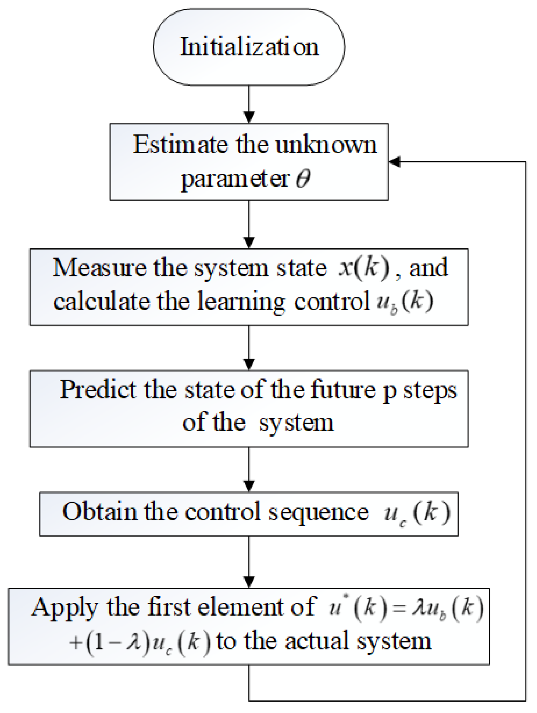
The algorithm is shown in the flowchart presented in Figure 2, detailed as follows:

• Initialize at time $k=0$ given the predictive horizon (p) and the stopping time N;
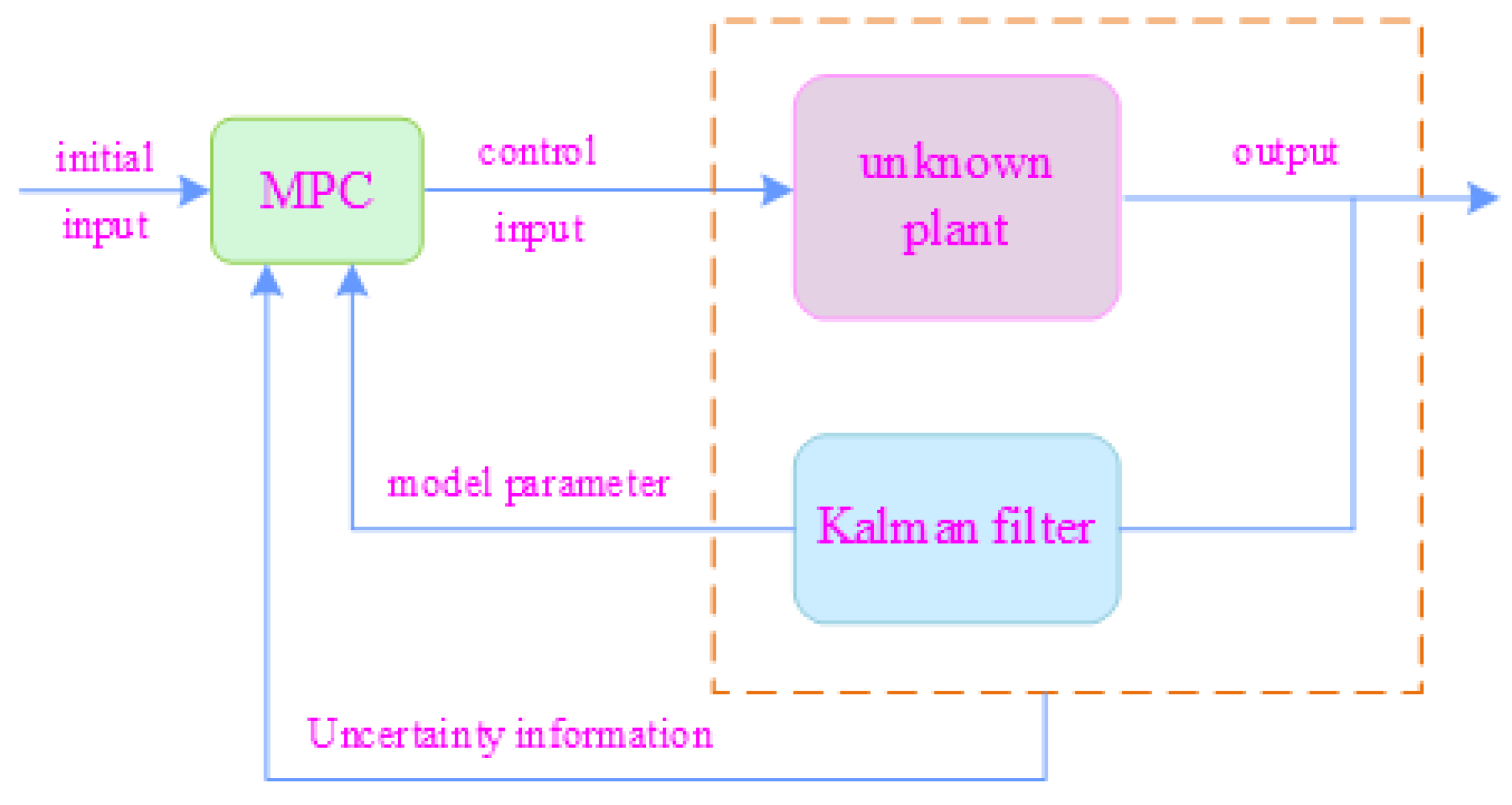
• Use the Kalman filter (i.e., (9)–(12)) to estimate the unknown parameter $\theta$;
• Measure the system state $x(k)$, and use (23) to calculate the learning control $u_b(k)$;
• The estimated state obtained via (20) predicts the state of the future p steps of the system;
• Solve the QP problem using (32) and obtain the control sequence $u_c(k)$;
• Apply the first element of $u^{*}(k)=\lambda u_b(k)+(1-\lambda )u_c(k)$ to the actual system;
• Set $k\leftarrow k+1$ and go to Step 1.

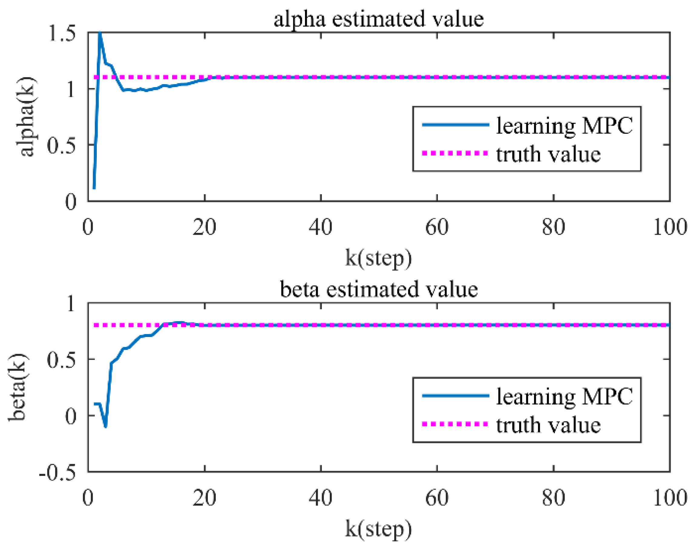
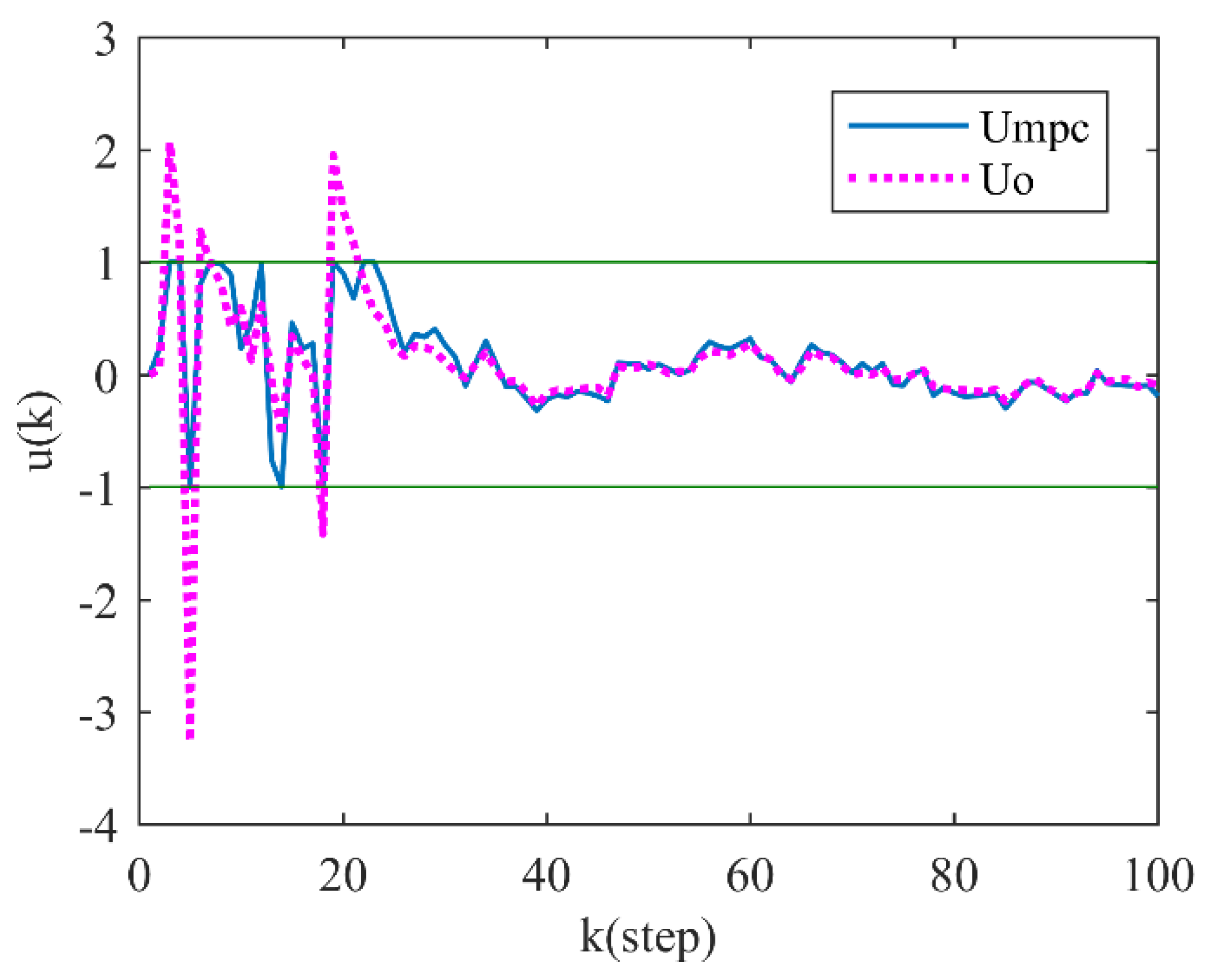
4.2. Simulation and Result Analysis

Consider the following stochastic systems:

$$x(k+1)=\alpha (k)x(k)+\beta (k)u(k)+v(k)$$

(36)

where $-1\le u(k)\le 1$.

Based on (4)–(6), this random system corresponds to

$$\left\{\begin{array}{c}x(k+1)={\phi }^T(k)\theta (k)+v(k)\\ \theta (k+1)=\theta (k)+\omega (k),\end{array}\right.$$

(37)

where $v(k)\sim N(0,0.04)$ and $\omega (k)={\left. [{\omega }_1(k){\omega }_2(k)\right]}^T$. The initial conditions are as follows: $\theta (0)={[1.1,0.8]}^T$, $\widehat{\theta }(0)={[0.1,0.1]}^T$, and $P(0)=diag[2,2]$, $x(0)=0.5$.

The system performance index is given as:

$$J=\underset{u}{min}\sum _{t=k}^{k+p-1}\left(x^T\left(t+1|k\right)Qx\left(t+1|k\right)+u^T(t)Gu(t)\right)$$

where the number of prediction steps is $p=10$, the number of system operation steps is $N=100$, and $Q=G=1$.

MATLAB was employed to simulate and verify the algorithm following the steps outlined in the previous section. This method can use the pre-estimated information to reduce the identification error for time-varying parameters as well as to effectively identify the unknown constant parameters.

The parameters in the model fluctuate randomly due to the influence of internal noise. As described, the learning effect is not evident. When the assumed model parameters’ variation equals zero $R_1=0$, the model parameters $\alpha$ and $\beta$ are constants. Here, $\alpha =1.1$, $\beta =0.8$.

Figure 3 shows the Kalman parameter estimation process during the control period. The solid line and dotted line in the figure are the estimated value and actual value of the parameter, respectively. It can be seen that the estimated and true value are close up to twenty steps, reflecting the speed and accuracy of the proposed learning algorithm.

Here, the optimal control sequence obtained with known parameters and no control constraints is compared with the MPC control sequence with learning characteristics. As shown in Figure 4, the MPC control sequence with learning characteristics is consistently better than the optimal control with known parameters before the system is identified. This result is due to the controller pursuing the control goal while learning the unknown parameters in the control process. After identifying the system’s real parameters, the MPC with learning characteristics closely tracks the optimal control with known parameters.

The optimal control sequence obtained with known parameters and no control constraints was compared with the MPC control sequence with learning characteristics as well. As shown in Figure 4, the MPC control sequence with learning characteristics is consistently better than the optimal control with known parameters before the system is identified. This result is due to the controller pursuing the control goal while learning the unknown parameters in the control process. After identifying the system’s real parameters, the MPC with learning characteristics closely tracks the optimal control with known parameters.

Generally speaking, it is difficult for the controller to learn the unknown parameters accurately, as small errors are inevitable, preventing MPC with learning characteristics from completely coinciding with the optimal control. In the simulation example, when the control time exceeds thirty time units, the MPC with learning characteristics almost coincides with the optimal control. Especially at steady state, the system can be considered to be running optimally.

Although the learning effect is evident when the system parameters are constant, it does not illustrate the algorithm’s capability to reduce the uncertainty in the future. When the model parameter variance changes, that is, $R_1\ne 0$, the model parameters $\alpha$ and $\beta$ take different values at every step, meaning that ${\omega }_1(k)\sim N(0,0.01)$ and ${\omega }_2(k)\sim N(0,0.001)$. Recall that $\lambda \in (0,1)$ in (34) is the learning factor. When $\lambda =0$, the control input in the system does not have any learning effect. In other words, in such a non-learning MPC, the uncertainty information is not utilized to reduce the system’s future uncertainty. The values $\lambda =0$ and $\lambda =0.5$ were used in the simulation, then the parameter estimation processes under these two learning factors were compared.

Figure 5 and Figure 6 show the estimation of parameters $\alpha$ and $\beta$ during the control period, which includes the true $\alpha$ and $\beta$ values, the non-learning MPC estimation process at $\lambda =0$, and the learning MPC estimation process at $\lambda =0.5$. It can be seen that the parameters obtained via the proposed MPC estimation with learning ability are closer to the ground truth when compared to the non-learning MPC’s parameter estimation process. Because the actual parameters in the model vary in time, even though the effect is obvious without learning constant parameters it can be seen that the error between the estimated value and the true value is decreasing. Therefore, the learned parameters become progressively more accurate, demonstrating that the algorithm effectively reduces the future uncertainty of the system.

Comparing the errors in the estimation process of the learning and non-learning MPCs, shown in Figure 7, it can be seen that the estimation error value of the learning MPC is near 0 and almost coincides with 0, while the error value of the non-learning MPC is always greater than that of the learning MPC.

To illustrate the improvement in system performance, we compare the control laws with a traditional adaptive MPC. Figure 8 and Figure 9 show the comparison between the optimal control law (obtained when all model parameters are known and there is no control constraint), the learning control law (obtained when the parameters are unknown and the control constraint is within the [−1, 1] range), the MPC1 control law (obtained with the algorithm in [10]) and the MPC2 control law (obtained with the algorithm in [16]). Because the system’s unknown parameters vary in time, the system needs to learn the unknown parameters at each time, and the control law does not reach a stable state. Furthermore, in addition to the control objectives, the dual controller needs to learn the unknown parameters. Consequently, the learning MPC control law is always greater than the optimal control law. However, when the parameter error gradually decreases in the later stage, the dual control law becomes closer to the optimal control law. Thus, when the system has uncertainty and the control algorithm with learning ability is used, the system runs in an approximately optimal manner. It can be seen from the figure that the method proposed in this paper is closer to the ideal control laws when the parameters are known, reflecting the superiority of the method as compared with the MPC1 and MPC2 control laws.

Table 1. Calculation time required for each MPC algorithm.

Control Model	Calculation Time
Optimal control law	1
Learning MPC	1.65
MPC1	1.41
MPC2	1.73

shows the calculation time required for each MPC algorithm:

Considering the high computation and performance requirements of dual MPCs, in order to test the real-time performance of the method proposed in this paper, the computation time of the above four control methods was compared at the same time. The optimal control law is set to a unit time, and the value is set to 1. By comparison, it can be seen that the method proposed in the paper consumes 65% more computing time than the optimal control laws, slightly more than MPC1 and slightly less than MPC2. Considering the development of embedded computers, the model prediction method studied in this paper has good prospects for application.

5. Discussion

This paper studied the MPC algorithm problem of a class of random linear discrete systems with unknown parameters, leading to the proposal of a controller with learning characteristics. The controller adds the best identification control component that minimizes the error variance of future estimates. Consequently, the algorithm enables learning the unknown parameters more accurately and controls the system to run in the direction required by the performance index. The weight factor is used to balance learning and control. However, the use of the learning process renders the control law derived in this paper sub-optimal. Thus, future studies should explore the weight factor settings to optimize the control and learning effect. Furthermore, it would be interesting to combine the advantages of the self-learning algorithm in this paper with the advantages of other adaptive algorithms for a system with gradually changing parameters.

References

1. Kikuchi, T.; Matsumoto, Y.; Chiba, A. Fast initial speed estimation for induction motors in the low-speed range. IEEE Trans. Ind. Inform. 2018, 54, 3415–3425. [Google Scholar] [CrossRef]
2. Xi, Y.; Li, D.; Lin, S. Model predictive control—Status and challenges. Acta Autom. Sin. 2013, 39, 222–236. [Google Scholar] [CrossRef]
3. Banholzer, S.; Fabrini, G.; Grüne, L.; Volkwein, S. Multiobjective Model Predictive Control of a Parabolic Advection-Diffusion-Reaction Equation. Mathematics 2019, 29, 4987–5001. [Google Scholar] [CrossRef]
4. Lorenzen, M.; Müller, M.A.; Allgöwer, F. Stochastic model predictive control without terminal constraints. Int. J. Robust Nonlinear Control 2019, 29, 4987–5001. [Google Scholar] [CrossRef]
5. Heirung, T.A.N.; Paulson, J.A.; Lee, S.J.; Mesbah, A. Model predictive control with active learning under model uncertainty: Why, when, and how. AIChE J. 2018, 64, 3071–3081. [Google Scholar] [CrossRef]
6. Mesbah, A. Stochastic model predictive control: An overview and perspectives for future research. IEEE Control Syst. 2016, 36, 30–44. [Google Scholar]
7. Campo, P.J.; Morari, M. Robust model predictive control. In Proceedings of the 1987 American Control Conference, Minneapolis, MN, USA, 10–12 June 1987; pp. 1021–1026. [Google Scholar]
8. Xie, L.; Xie, L.; Su, H. A comparative study on algorithms of robust and stochastic MPC for uncertain systems. Acta Autom. Sin. 2017, 43, 969–992. [Google Scholar]
9. Zhang, K.; Yang, S. Adaptive model predictive control for a class of constrained linear systems with parametric uncertainties. Automatica 2020, 117, 108974. [Google Scholar] [CrossRef]
10. Zhang, S.; Dai, L.; Xia, Y. Adaptive MPC for constrained systems with parameter uncertainty and additive disturbance. IET Control Theory Appl. 2019, 13, 2500–2506. [Google Scholar] [CrossRef]
11. Ding, B.; Pan, H. Output feedback robust MPC for LPV system with polytopic model parametric uncertainty and bounded disturbance. Int. J. Control 2016, 89, 1554–1571. [Google Scholar] [CrossRef]
12. Pipino, H.A.; Adam, E.J. MPC for linear systems with parametric uncertainty. In Proceedings of the 2019 XVIII Workshop on Information Processing and Control, Salvador, Brazil, 18–20 September 2019; pp. 42–47. [Google Scholar]
13. Dhar, A.; Bhasin, S. Indirect adaptive mpc for discrete-time lti systems with parametric uncertainties. IEEE Trans. Automat. Contr. 2021, 66, 5498–5505. [Google Scholar] [CrossRef]
14. Liu, J.; Jayakumar, P.; Stein, J.L.; Ersal, T. Improving the robustness of an MPC-based obstacle avoidance algorithm to parametric uncertainty using worst-case scenarios. Veh. Syst. Dyn. 2019, 57, 874–913. [Google Scholar] [CrossRef]
15. Adetola, V.; DeHaan, D.; Guay, M. Adaptive model predictive control for constrained nonlinear systems. Syst. Control Lett. 2009, 58, 320–326. [Google Scholar] [CrossRef]
16. Gonçalves, G.A.A.; Guay, M. Robust discrete-time set-based adaptive predictive control for nonlinear systems. J. Process Control 2016, 39, 111–122. [Google Scholar] [CrossRef]
17. Mesbah, A. Stochastic model predictive control with active uncertainty learning: A Survey on dual control. Annu. Rev. Control 2018, 45, 107–117. [Google Scholar] [CrossRef]
18. Shang, T.; Qian, F.; Zhang, X.; Xie, G. Research on dual control algorithm for LQG with unknown parameters. Acta Autom. Sin. 2017, 43, 1478–1484. [Google Scholar]
19. Yang, H.; Gao, S.; Qian, F. A suboptimal Dual Control Method for the Stochastic Systems with Parameters Drifting. Asian J. Control 2019, 21, 609–616. [Google Scholar] [CrossRef]
20. Heirung, T.A.N.; Ydsite, B.E.; Foss, B. Dual adaptive model predictive control. Automatica 2017, 80, 340–348. [Google Scholar] [CrossRef]
21. Houska, B.; Tenlen, D.; Logist, F.; Impe, J.V. Self-reflective model predictive control. SIAM J. Control Optim. 2016, 55, 2959–2980. [Google Scholar] [CrossRef]
22. Feng, X.; Houska, B. Real-time algorithm for self-reflective model predictive control. J. Process Control 2018, 65, 68–77. [Google Scholar] [CrossRef]
23. Zeng, J.; Liu, J. Distributed State Estimation Based Distributed Model Predictive Control. Mathematics 2021, 9, 1327. [Google Scholar] [CrossRef]
24. Cao, W.; Li, S. Enhanced parameterizable uncertainty to dual adaptive model predictive control. Control Theory Appl. 2019, 36, 1197–1206. [Google Scholar]
25. Chen, H. Model Predictive Control; Science Press: Beijing, China, 2013; pp. 161–165. [Google Scholar]
Figure 1. Block diagram of MPC with learning characteristics.
Mathematics 10 03152 g001
Figure 2. Flow diagram of the algorithm.
Mathematics 10 03152 g002
Figure 3. Estimated and true values when parameters α ( k ) and β ( k ) are constant.
Mathematics 10 03152 g003
Figure 4. Comparison of optimal MPC and learning MPC control signals when parameters are constant.
Mathematics 10 03152 g004
Figure 5. Estimated and true α ( k ) values when the parameter varies with time.
Mathematics 10 03152 g005
Figure 6. Estimated and true β ( k ) values when the parameter varies with time.
Mathematics 10 03152 g006
Figure 7. Estimated error of parameters α ( k ) and β ( k ) .
Mathematics 10 03152 g007
Figure 8. Comparison of various MPC control laws.
Mathematics 10 03152 g008
Figure 9. Partial comparison of various MPC control laws.
Mathematics 10 03152 g009