Article

ADMM-Based Differential Privacy Learning for Penalized Quantile Regression on Distributed Functional Data

School of Statistics and Data Science, Nanjing Audit University, Nanjing 211085, China
*
Author to whom correspondence should be addressed.
Mathematics 2022, 10(16), 2954; https://doi.org/10.3390/math10162954
Submission received: 25 July 2022 / Revised: 10 August 2022 / Accepted: 12 August 2022 / Published: 16 August 2022
(This article belongs to the Special Issue Statistical Modeling for Analyzing Data with Complex Structures)

Abstract

:
Alternating Direction Method of Multipliers (ADMM) is a widely used machine learning tool in distributed environments. In the paper, we propose an ADMM-based differential privacy learning algorithm (FDP-ADMM) on penalized quantile regression for distributed functional data. The FDP-ADMM algorithm can resist adversary attacks to avoid the possible privacy leakage in distributed networks, which is designed by functional principal analysis, an approximate augmented Lagrange function, ADMM algorithm, and privacy policy via Gaussian mechanism with time-varying variance. It is also a noise-resilient, convergent, and computationally effective distributed learning algorithm, even if for high privacy protection. The theoretical analysis on privacy and convergence guarantees is derived and offers a privacy–utility trade-off: a weaker privacy guarantee would result in better utility. The evaluations on simulation-distributed functional datasets have demonstrated the effectiveness of the FDP-ADMM algorithm even if under high privacy guarantee.

1. Introduction

Machine learning is becoming more and more common in statistical modeling and data analysis, along with the increasing concerns about the privacy disclosure of data. Therefore, we urgently need to develop algorithms which can provide privacy protection for personal data. In turn, the demand for data privacy protection has stimulated the establishment of formal standards on data privacy and the development of privacy framework. Among them, differential privacy (DP) [1,2] is the most widely discussed and developed technique in theory [3,4,5,6], and the feasibility of adopting these theories is shown among others by [7,8,9]. The framework of DP makes it convenient for us to construct privacy protection algorithms. However, these privacy protection algorithms may also need to pay a price of sacrificing the rate of convergence in statistical accuracy. Therefore, we need to develop differential privacy distributed learning algorithms that do not sacrifice statistical accuracy as much as possible for large-scale distributed data.
Distributed machine learning can disassemble the original huge training task into multiple sub-tasks, that is, transforming large-scale learning that one machine can not afford during collaborative learning with multiple machines. Recently, ref. [10] gave a sparse distributed learning solution for high-dimensional problems; ref. [11] proposed a distributed learning algorithm which segments features in a high-dimensional sparse additive model and proved the consistency of the sparse patterns for each additive component; ref. [12] provided a more flexible framework using the communication-efficient surrogate likelihood (CSL) procedure, which can solve different settings such as M-estimation for low- and high-dimensional problems and Bayesian inference. Ref. [13] extended the CSL method to distributed quantile regression and then established some statistical properties under quantile loss, which does not satisfy the smoothness condition of CSL method. In distributed learning, each sub-task is executed separately on an independent machine. It allows each machine to complete a collective learning objective, which is usually a standardized empirical risk minimization problem. The individual data that do not need to be disclosed will be calculated in a local iterative algorithm, and the parameters will be transferred between the central machine and each local machine. At present, the widely used algorithms for the decentralized distributed learning problems mainly include subgradient-based algorithms [14,15], alternating direction method of multipliers(ADMM) [16,17,18,19], and the combination algorithms of these methods [20]. Ref. [21] proved that ADMM-based algorithms converge at the rate of O ( 1 / L ) , while subgradient-based algorithms usually converge at the rate of O ( 1 / L ) , where L is the number of iterations. Therefore, in this paper, we adopt an ADMM-based distributed learning algorithm against privacy disclosure and keep a statistical guarantee.
We know that sensitive individual information may be leaked in optimization algorithms as a result of sharing information such as parameters and/or gradients of the model between machines, as presented in [22,23]. The same problem exists in our ADMM-based distributed algorithm: how to avoid privacy leakage. So, we need to protect privacy via a DP mechanism while maintaining statistical accuracy in our distributed learning. Ref. [24] studied a class of regularized empirical risk minimization machine learning problems via ADMM and proposed the dual variable perturbation and the primal variable perturbation methods for dynamic differential privacy. Ref. [25] proposed a privacy-preserving cooperative learning scheme, where users are allowed to train independently using their own data and only share some updated model parameters. They used an asynchronous ADMM approach to accelerate learning. In addition, their algorithm integrates secure computing and distributed noise generation to ensure the confidentiality of shared parameters during the asynchronous ADMM algorithm process. Ref. [26] applied a new privacy-preserving distributed machine learning (PS-ADMM) algorithm based on stochastic ADMM, which provides a privacy guarantee by perturbing the gradient and has a low computational cost. In the paper, we focus on a functional linear regression model for functional data analysis via ADMM-based distributing learning to keep DP and statistical efficiency.
Functional data are natural generalizations of multivariate data from finite dimensional to infinite dimensional which are obtained by observing a number of subjects over time, space, and other continua. In practice, functional data are frequently recorded by an instrument, which involves a large number of repeated measurements per subject. They can be curves, surfaces, images, or other complex objects; see some real data sets in the monographs [27,28,29]. All in all, a functional datum is not a single observation but rather a set of measurements along a continuum; taken together, they are regarded as a single entity, curve, or image. In recent decades, functional data analysis has drawn considerable attention because advanced technology makes functional data easier to collect in applied fields such as medical studies, speech recognition, biological growth, climatology, online auctions, and so on. Time series data are treated as multivariate data because they are given as a finite discrete time series. In addition, longitudinal data, which are often observed in biomedical follow-up studies, are strongly linked with functional data; however, their use often involves several (few) measurements per subject taken intermittently at different time points for different subjects. Therefore, functional data and longitudinal data are also intrinsically different. In addition, some classic multivariate data analysis tools, applied to time series and longitudinal data analysis, cannot be directly applied to functional data analysis because they ignore the fact that the underlying object of the measurements of a subject is a function such as curve or surface. We know that functional data are intrinsically infinite dimensional, and our analysis methods cannot be based on the assumption that the values observed at different times for a single subject are independent because of the intra-observation dependence. The high intrinsic dimensionality and the intra-observation dependence of functional data pose challenges both for theory and computation.
Recently, various approaches and statistical models for the analysis of functional data have been developed. For an introduction and summary, see [27,28,29,30]. Ref. [31] firstly proposed a linear regression model and analyzed the effects of functional independent variables on the scalar response variables through the inner product of functional independent variables and unknown nonparametric coefficient function. Ref. [32] gave a functional linear semiparametric quantile regression model, which has been used to analyze ADHD-200 patients data. Ref. [33] studied the estimation problem of a functional partial quantile regression model, and proved the asymptotic normality of the finite dimensional parameter estimation. The conventional method of functional data analysis is principal component analysis (PCA), such as [34,35]. Ref. [35] gave the optimal convergence rates of PCA. We will consider functional principal components analysis (FPCA) for our functional linear regression model and investigate the distributed learning with privacy.
In this paper, we propose a new ADMM-based distributed learning algorithm with differential privacy to handle large amounts of functional data. We call it the FDP-ADMM algorithm. Our proposed FDP-ADMM algorithm has good properties such as a faster rate of convergence, lower communication and computation costs, and better utility–privacy tradeoffs. In the FDP-ADMM algorithm, we consider a more robust quantile loss function, combine an approximate augmented Lagrange function, and integrate time-varying Gaussian noise into local learning on each machine. These techniques allow the FDP-ADMM algorithm to be adversarial while protecting privacy.
The main contributions of this paper are summarized as follows:
  • We propose a distributed learning algorithm (FDP-ADMM) that can process large-scale distributed functional data and protect privacy. For the large-scale functional data, we adopt functional principal component analysis to reduce the dimensions of the data, improve the quality of data information, and promote the efficiency of functional data analysis using distributed learning.
  • We introduce a quantile loss function for functional linear model such that our models are adaptive to heavy-tail data or outliers. Thus, our ADMM-based distributed learning algorithm is more robust compared with ordinary least square procedure.
  • The privacy and theoretical convergence guarantees of the FDP-ADMM algorithm are derived, and a privacy–utility trade-off is demonstrated: a weaker privacy guarantee would result in better utility.
  • We conduct numerical experiments to illustrate the effectiveness of FDP-ADMM in the framework of distributed learning. The results of experiments are consistent with our theoretical analysis.
The rest of this paper, is organized as follows. In Section 2, we state our problem formulation by introducing the functional linear regression model, the penalized quantile regression, the ADMM algorithm, and DP. In Section 3, we propose an ADMM-based distributed learning algorithm with privacy protection for distributed functional data analysis. In Section 4, we present the utility analysis of our algorithm, FDP-ADMM, including the convergence and privacy guarantee. In Section 5, we give some numerical experiments to verify our theoretical results. Some conclusions are given in Section 6. The proofs of the main results are collected in Appendix A.

Notations

For any positive integer n, we define [ n ] : = { 1 , 2 , , n } . · , · 2 and · are denoted as the Euclidean norm, 2 -norm, and -norm, respectively. ρ τ ( u ) = u ( τ I { u 0 } ) is the quantile loss function for a scalar u R . and I { · } denotes the indicator function. For a vector u = ( u 1 , , u n ) T , we define ρ τ ( u ) = i = 1 n ρ τ ( u i ) . Throughout this paper, the constant C denotes positive constant whose value may change from line to line. For any function f and a positive function ϕ , f ϕ means a ϕ < f < b ϕ for some positive constants a and b.

2. Problem Formulation

In this section, we present the functional data model, quantile regression, ADMM algorithm, and difference privacy mechanisms to be studied.

2.1. Functional Data Analysis

Functional data consist of functions that are basically smooth but are usually corrupted with noise, such as curves, images, and so on. For simplicity, we assume the functional predictor X ( t ) on the finite time interval I = [ 0 , T ] . Let x i ( t ) : t I 1 i n be observation variables; that is, for each t I , there exists an observed value x i ( t ) R . A typical functional data set is:
x i t j , i R : t j , i I , 1 i n , 1 j J i ,
where J i is the observation number, and n is the number of individuals. If J i is small, then the data are called sparse; otherwise they are called dense. FDA pays attention to the shape of the potential function or curve of the data via some statistical models and estimation procedures.
Functional linear regression is a standard method in functional data analysis for incorporating functional predictors, which focuses on modeling the relationship between a functional or continuous response Y and a functional predictor X ( t ) , in which t varies in a compact set I. It usually has the form:
Y = β 0 + I β ( t ) X ( t ) d t + ϵ ,
where β 0 is a intercept term, ϵ is the random noise independent of X ( t ) , and β ( t ) is an unknown function of interest. Without loss of generality, we assume E ( Y ) = 0 and E ( X ( t ) ) = 0 . Based on data { ( X i ( t ) , Y i ) , i = 1 , , n } , the model becomes:
Y i = I β ( t ) X i ( t ) d t + ϵ .
FPCA is commonly used for analyzing such models (1) with the purpose of dimension reduction. The main idea is to summarize the data variation and information via some dimensional loadings. Dimension reduction in FPCA is performed through an expansion of basis, which consists of the eigenfunctions formed by the covariance operator Σ ( · , · ) of the process X ( t ) : t I . By Mercer’s theorem, the spectral decomposition is
Σ ( s , t ) = C o v ( X ( s ) , X ( t ) ) = k = 1 λ k ϕ k ( s ) ϕ k ( t ) ,
where s , t I , λ k are the ordered eigenvalues such that λ 1 λ 2 , and the function ϕ k forms the orthogonal basis corresponding to λ k , k = 1 , 2 , .
By Karhunen and Loève [36], in the classical functional principal component analysis, the ith random curve X ( t ) and functional coefficient β ( t ) can be expressed as:
X i ( t ) = k = 1 A i k ϕ k ( t ) , β ( t ) = k = 1 w k ϕ k ( t ) ,
where the coefficients A i k = I X i ( t ) ϕ k ( t ) d t and w k = I β ( t ) ϕ k ( t ) d t are the functional principal components. In addition, E A i k = 0 and var A i k = λ k for k = 1 , 2 , . We have the top K of λ k and taking their corresponding ϕ k ( t ) , we have an approximation to X i ( t ) truncated as:
X i K ( t ) = k = 1 K A i k ϕ k ( t ) .
Then we consider the functional principal component regression into the functional linear model:
Y i = I X i ( t ) β ( t ) d t + ϵ i k = 1 K A i k w k + ϵ , f o r i = 1 , , n ,
We regard w k ( k = 1 , , K ) as unknown parameters. We can select a proper K FPCA basis to represent the functional data X i ( t ) ; that is, the most important information of data can be refined by FPCA.

2.2. Quantile Regression with Penalties

We have i.i.d observations ( A i , y i ) , i = 1 , 2 , , n , with A i = ( A i 1 , , A i K ) . Let Q y i A i ( τ ) = A i w τ be the conditional quantile of y i on A i R K , for a give the quantile level τ th, τ ∈(0,1). Let w τ = w 1 , τ , , w K , τ T . The quantile regression estimate of w τ is defined as:
w ^ τ = arg min w R K ρ τ ( y A w ) ,
where A = A 1 , A n T R n × K is a matrix, ρ τ ( u ) = u ( τ I { u 0 } ) is the quantile loss function for a scalar u R and I { · } denotes the indicator function.
Penalized quantile regression (PQR) is formulated as
min w ρ τ ( y A w ) + P λ w ,
where P λ ( · ) is a penalty, such as lasso penalty [37],
P λ w = λ w 1 ;
or elastic net [38],
P λ w = λ λ 2 w 2 2 + λ 1 w 1 , λ 1 , λ 2 0 .
Penalized QR, such as (5) and (6), leads to biased estimators. To obtain an unbiased estimator, refs. [39,40] proposed a non-convex penalty, for instance, the MCP penalty [39], or the SCAD penalty [40].
Our learning empirical loss is:
L ^ ( w ) : = 1 n i = 1 n ρ τ y i A i w
based on all data coming from all machines. As the data are distributed on local machines, it is difficult to collect all data into one machine, and additionally, there are privacy issues. Therefore, we apply the technique of distributed learning via the ADMM algorithm for the following distributed empirical loss (11). ADMM is a computational framework to solving optimization problems.

2.3. ADMM Algorithm

ADMM algorithm was first proposed by [41,42] in 1975 and 1976, respectively. Then, ADMM was reviewed and proven to be suitable for large-scale distributed optimization by [16]. In this section, we give the basic ADMM formulation.
Assume that our optimization problem is expressed as:
min x , z { f ( x ) + g ( z ) } s . t . B x + C z = d
where x R n , z R s , matrices B R m × n and C R m × s , vector d R m , and functions f : R n R and g : R s R . x and z are the variables needing to be optimized. The optimization problem (8) consists of two parts: f ( x ) related to variable x and g ( z ) related to variable z. This structure can easily be dealt with via ADMM as follows: First, we have the augmented Lagrangian function:
L ρ ( ( x , z ) , u ) : = f ( x ) + g ( z ) + u T ( B x + C z d ) + ρ 2 B x + C z d 2 2 ,
where u is the dual variable (or called the Lagrange multiplier), and ρ > 0 is a penalty parameter. The name ‘augmented’ in the L ρ refers to the quadratic penalty term ρ 2 B x + C z d 2 2 , which is added for better convergence properties of algorithm. Then, the ADMM iterative solution of the optimization problem (9) is:
x l + 1 : = arg min x L ρ x , z l , u l , z l + 1 : = arg min z L ρ x l + 1 , z , u l , u l + 1 : = u l + ρ B x l + 1 + C z l + 1 d .
The ‘multiplier method’ in ADMM refers to a dual ascent using augmented Lagrange function (with quadratic penalty term), and the ‘alternating direction’ refers to variables x and z be updated alternately. For more theories and applications about ADMM, refer to [16].

2.4. Differential Privacy

Differential privacy technology was originally designed to confront differential attacks problem. The traditional protecting method is to anonymize or encrypt to the datasets. However, some individual information can still be recovered from these anonymous data, based on certain algorithms, such as the recommendation algorithm. Therefore, Ref. [3] proposed the mechanism of differential privacy to protect privacy, which adds a designed noise in the algorithm so that attackers can not recover data information. Moreover, it has been proven that as long as the noise satisfies the differential privacy mechanism, no matter how much prior information the attacker has, the anonymous data cannot be reconstructed.
This paper mainly studies differential privacy for ADMM against adversarial attacks. Intuitively speaking, if an adversary can not tell whether a individual datum x belongs to the special data set X or not, when we output results from algorithm M ( X ) . We call that DP. Now, we give the definition of the ( ϵ , δ ) -differential privacy from Dwork’s work [2].
Definition 1
( ( ϵ , δ ) -Differential Privacy). A randomized algorithm M : X n R is ( ϵ , δ ) -differential private if for any two adjacent datasets (differing in only one tuple) X, X X n , and for any measurable output subset S range ( M ) :
P [ M ( X ) S ] e ϵ · P M X S + δ ,
where probability measure P , which is bounded, only depends on the randomness of algorithm M .
In Definition 1, δ and ϵ measure the protection strength of the privacy. It implies that a smaller δ or a smaller ϵ gives better privacy protection. The Laplace and Gaussian mechanisms are two typical methods that are widely used in ( ϵ , δ ) -differential privacy. They offer calibrated noise sampled from Laplace or Gaussian distribution, and add this noise into the algorithm. Now we consider a class of deferentially private algorithms via compositions, termed ‘k-fold adaptive composition’ in the literature. The advanced composition stated below, where the auxiliary inputs of the k-th algorithm are the outputs of all previous algorithms, shows how privacy parameters degrade as private algorithms are composited.
Lemma 1
(Theorem 4 in [43] (Advanced Composition)). Let ϵ , δ 0 . The class of ( ϵ , δ ) -differentially private algorithms satisfies ϵ , δ -differential privacy under k-fold adaptive composition, where ϵ = c 0 k ϵ for some constant c 0 .

3. Distributed Learning with DP for Functional Data via ADMM

In this section, we propose the ADMM-based distributed learning algorithm with DP for functional data, which is called FDP-ADMM. We will transfer the functional regression model (1) into a linear regression model (2) by using FPCA. Because quantile regression has better performance in estimation and prediction for non-Gaussian distribution error, such as heavy-tailed distribution or outliers, we consider quantile regression for the models (1) and (2). First, based on data { ( X i ( t ) , y i ) , i = 1 , , n } , the functional quantile linear regression model we consider is
y i = I β τ ( t ) X i ( t ) d t + ϵ τ , i ,
where τ ( 0 , 1 ) is a given quantile level, and ϵ τ , i are random errors. Without loss of generality, we assume that the τ th quantile of ϵ τ , i is equal to zero. The model can be written as Q y i | X i ( τ ) = I β τ ( t ) X i ( t ) d t . Our goal is to learn the functional coefficient β τ ( t ) by
min β τ ( t ) i = 1 n ρ τ y i I β τ ( t ) X i ( t ) d t .
The problem is difficult because of the term I β τ ( t ) X i ( t ) d t . By the FPCA introduced in Section 2.1, we have the model (2):
y i = I X i ( t ) β τ ( t ) d t + ϵ τ , i k = 1 K A i k w τ , k + ϵ τ , i , f o r i = 1 , , n .
That is, functional quantile linear regression is transformed as an ordinary quantile linear regression. We suppress the dependency of w τ , k on τ for simplicity. Then, for the quantile linear regression, we propose penalized quantile regression learning, which is formulated as
min w ρ τ ( y A w ) + P λ w .
It has been introduced in Section 2.2.
However, our dataset { ( X i ( t ) , y i ) , i = 1 , , n } cannot be collected on one machine, but distributed over M machines. That is, we have the distributed data { ( X i , j ( t ) , y i , j ) , i = 1 , , M , j = 1 , , m i } , where M is the number of worker machines, and m i is the size of sample on the ith machine. Thus, based on FPCA, { ( X i , j ( t ) , y i , j ) , i = 1 , , M , j = 1 , , m i } is transformed as { ( y i j , A i , j ) , i = 1 , , M , j = 1 , , m i } , where A i , j = ( A i , j 1 , , A i , j K ) is the score of the jth sample on the ith worker machine. So, based on the distributed data { ( y i j , A i , j ) , i = 1 , , M , j = 1 , , m i } and the model (2), we have the following QR estimation in the distributed framework:
w ^ τ = argmin i = 1 M j = 1 m i 1 m i ρ τ y i j A i , j w ,
where ρ τ ( · ) is the loss function of quantile regression, and w is the unknown coefficient. Furthermore, we modify QR as penalized QR estimator for achieving faster shrinking, that is:
w ^ τ = argmin i = 1 M j = 1 m i 1 m i ρ τ y i j A i , j w + P λ ( w ) .
Note that in (12), there exist two type of tuning parameters, K and λ , where K controls the number of scores to characterize the decomposition level of FPCA and λ controls the fitness of the model.
When facing big data, that is, when n is very large, it is hard for one machine to learn w in (12). So, it is necessary to distributed storage and learning. Next, we will demonstrate the ADMM-based distributed learning for penalized QR. We provide a sketch of our FDP-ADMM algorithm based on the distributed data.

3.1. ADMM-Based Distributed Learning Algorithm

Assume we have M machines, and the ith machine has m i local data samples. Applying the ADMM algorithm, we re-formulate the problem (12) as:   
min w i i [ M ] i = 1 M j = 1 m i 1 m i ρ τ y i j A i , j w i + λ M P w i , s . t . w i = w , i = 1 , , M ,
where w i R K is the local model parameters, and w R K is the global ones. Then, the augmented Lagrangian function for the ith machine is:
L ρ , i w i , w , γ i = j = 1 m i 1 m i ρ τ y i j A i , j w i + λ M P w i γ i , w i w + ρ 2 w i w 2
s . t . w i = w , i = 1 , 2 , , M .
The objective (14) is decoupled and each worker only needs to minimize the sub-problem based on its local data set. Constraints (15) enforce all the local models to consensus. It results in the following iteration:
w i l = argmin w i L ^ ρ , i w i , w l 1 , γ i l 1 ,
w l = 1 M i = 1 M w i l 1 M i = 1 M γ i l 1 / ρ ,
γ i l = γ i l 1 ρ w i l w l .
Note that each machine transfers its w i l , γ i l to a central machine. The central machine gathers them to update w l and then broadcasts it to each machine. Details for the algorithm are present in Algorithm 1. Based on output w L , we obtain:
β ^ N D P ( t ) = k = 1 K w k L ϕ k ( t ) .
Algorithm 1:ADMM for PQR of Functional Data (F-ADMM)
Mathematics 10 02954 i001

3.2. ADMM-Based Distributed Learning with DP

For achieving faster optimization, we make use of the first-order approximation to the penalized objective function. Then, L ρ , i w i , w , γ i in (14) becomes:
L ^ ρ , i w i , w ˜ i l 1 , w , γ i = j = 1 m i 1 m i ρ τ y i j A i , j w ˜ i l 1 + λ M P w ˜ i l 1 + j = 1 m i 1 m i ρ τ y i j A i , j w ˜ i l 1 + λ M P w ˜ i l 1 , w i w ˜ i l 1 γ i , w i w + ρ 2 w i w 2 + w i w ˜ i l 1 2 2 η i l ,
where η i l R is the time-varying step size which decreases as the iteration l grows, ρ τ is the subgradient of the quantile loss function, and P is the subgradient of the penalty. So, we have the following optimization problem:
min w i i = 1 M L ^ ρ , i w i , w ˜ i l 1 , w , γ i s . t . w i = w , i = 1 , 2 , , M .
Here, we give the ADMM-based distributed learning algorithm with DF (FDP-ADMM) as follows:
w i l = argmin w i L ^ ρ , i w i , w ˜ i l 1 , w l 1 , γ i l 1 ,
w ˜ i l = w i l + ξ i l ,
w l = 1 M i = 1 M w ˜ i l 1 M i = 1 M γ i l 1 / ρ ,
γ i l = γ i l 1 ρ w ˜ i l w l ,
where ξ i l in (22) are sampled from N 0 , σ i , l 2 I K , and w l in (23) is computed on the central machine. The rest are processed at each local machine. Details on FDP-ADMM algorithm are presented in Algorithm 2. Based on output w L of Algorithm 2, we obtain:
β ^ D P ( t ) = k = 1 K w k L ϕ k ( t ) .
Note that the central machine initializes the global w 0 , while each worker machine initializes their own variables: the noisy primal variables w ˜ i 0 and the dual variables γ i 0 for i [ M ] . ξ i l is Gaussian noise with zero-mean and variance σ i , l 2 , where σ i , l 2 is obtained based on the Gaussian mechanism of DP, which is given in Theorem 1. Each worker machine updates its noisy primal variable w ˜ i l based on (22). Then, the central machine receives all noisy primal variables w ˜ i l i [ M ] and the dual variables γ i l i [ M ] from the worker machine, and updates a global variable w l . In addition, w l on central machine broadcasts to every worker machine to update the final dual variables γ i l i [ M ] using (24). It is an iterative cycle.
We set the variance σ i , l = 2 c 1 2 ln ( 1.25 / δ ) m i ϵ ρ + 1 / η i l for obtaining the ( δ , ϵ ) -DP of the FDP-ADMM algorithm, which is set based on the Gaussian mechanism of DP. σ i , l 2 is time-varying; that is, it decreases as iteration l increases. The motivation of using time-varying variance in the Gaussian mechanism is to reduce the negative impact of noise and ensure the convergence of the algorithm. We find that the negative impact will be mitigated by the method of decreasing noise and can achieve a stable solution.
For the communication and computation costs of our algorithms 1 and 2, here are some remarks. We know that it is unrealistic to send the estimator of β ( t ) , t [ 0 , 1 ] on a worker machine to the central machine because it is infinite dimensional. In Algorithms 1 and 2, we only transmit the K-dimensional w in each round of communication, so the communication complexity is only O ( K ) . In practice of functional data analysis, K is usually a small number such as 5, 10, etc. Therefore, our algorithms are communication-efficient because of the low communication costs. In addition, in each round of learning, each worker machine learns its own low-dimensional parameter w based on its local data, then the central machine is responsible for summarizing these parameters from worker machines. This working mechanism greatly reduces the computational costs.    
Algorithm 2:ADMM-based distributed learning with DP for PQR of Functional Data (FDP-ADMM)
Mathematics 10 02954 i002

4. Utility Analysis

4.1. Privacy Guarantee

In the section, we will analyze the privacy guarantee of the proposed FDP-ADMM algorithm. During traditional parameter transmission, the shared information w i l l [ L ] can divulge the sensitive messages of original data. So, it is necessary to show outputs w ˜ i l l [ L ] with differential privacy.
Denote the two neighboring datasets A i and A i . So, the w i , A i l and w i , A i l are the primal variables obtained from every local worker machine. From the FDP-ADMM algorithm, we add noise to w i l by Gaussian mechanism. A fundamental tool used in DP is sensitivity. We use l 2 -norm sensitivity. Due to the application of first-order approximation in the augmented Lagrange function, the proposed algorithm does not require the smoothness and strong convexity assumptions to the objective function for proving the sensitivity.
First, we give a lemma, which gives an l 2 -norm sensitivity of w i l under the sub-gradient of loss function , bounded.
Lemma 2.
Assume that ( · ) 2 c 1 . The l 2 -norm sensitivity of the local primal variable w i l update function is given by:
max A 1 , A 1 w i , A i l w i , A i l = 2 c 1 m i 2 ρ + 1 / η i l .
Its proof is given in Appendix A. Lemma 2 shows that the l 2 sensitivity of w i l is affected by the time-varying η i l . We set η i l as a decreasing function of l, so the l 2 sensitivity decreases with increasing l. That is, if ϵ and δ is fixed, the added noise in the proposed algorithm will become smaller as the l increases. Therefore, the algorithm will be stably convergent in spite of adding the noise. Then, we show that Algorithm 2 guarantees ( ϵ , δ ) -differential privacy.
Theorem 1.
Assume that >A i j 2 c 1 , i = 1 , , M and j = 1 , , m i in the model (11). Let ϵ ( 0 , 1 ] be arbitrary and ξ i k be the noise sampled from Gaussian mechanism with variance σ i , k 2 , where
σ i , k = 2 c 1 2 ln ( 1.25 / δ ) m i ϵ ρ + 1 / η i k .
The FDP-ADMM guarantees ( ϵ , δ ) -differential privacy. Specifically, for any neighboring datasets A i and A i , for any output w ˜ i k , the following inequality always holds:
Pr w ˜ i k A i e ϵ · Pr w ˜ i k A i + δ .
Its proof is given in Appendix A.

4.2. Convergence of the FDP-ADMM Algorithm

The convergence of ADMM for convex problems has been widely studied in recent years. Under the requirement of high precision, the convergence of ADMM goes very slowly. However, under the requirement of medium precision, the convergence speed of ADMM is acceptable, and the global solution can be achieved by dozens of iterations. Furthermore, Ref. [44] showed that ADMM could attain a global linear convergence on strict convexity and Lipschitz gradient, especially when matrix B and C in (8) are full column rank. The ADMM framework is suitable for large-scale statistical learning problems. More convergence analysis of ADMM under convexity were studied by [45,46,47,48,49,50,51,52], and so on. Ref. [53] proposed an approximate ADMM algorithm to make it converge to the stable point with a large enough penalty parameter. Ref. [54] gave the convergence of quantile regression using ADMM for convex and non-convex penalties. We refer to [54] for the convergence of our FDP-ADMM algorithm.
We define w * as the optimal solution of (13) and c w = w * 2 . The convergence of the algorithm is based on the fact that the quantile loss function is convex and non-smooth. For simplicity of analysis, we define some notations as follows:
f i w i = j = 1 m i 1 m i ρ τ y i j A i , j w i + λ M P w i , w ¯ L = 1 L l = 1 L w l , γ ¯ i L = 1 L l = 1 L γ i l , w ¯ i l = 1 L l = 0 L 1 w ˜ i l , u i l = w ˜ i l w l γ i l , u i = w i w γ i , F u i l = γ i l γ i l w ˜ i l w l .
We analyze the convergence of our proposed algorithm in terms of both the objective value and the constraint violation as [55]:
i = 1 M f i w ¯ i L f i w * + g w ¯ i L w ¯ L ,
where i = 1 M f i w ¯ i L f i w * is used to measure the distance between the current objective value and the optimal value, and i = 1 M g w ¯ i L w ¯ L depicts the difference between the local model and the global one. If the training result of our FDP-ADMM algorithm achieves optimal and local models, it obtains consensus.
Lemma 3
([55], lemma 2). Assume ρ τ ( · ) and P ( · ) are convex. For any l 1 , we have:
i = 1 M f i w ˜ i l 1 f i w i + u i l u i F u i l i = 1 M η i l 2 f i w ˜ i l 1 ρ + 1 / η i l ξ i l 2 ρ 2 w i w l 2 + ρ 2 w i w l 1 2 ρ + 1 / η i l ξ i l , w i w ˜ i l 1 + 1 2 η i l w i w ˜ i l 1 2 1 2 η i l w i w ˜ i l 2 + 1 2 ρ γ i γ i l 1 2 1 2 ρ γ i γ i l 2 .
Based on Lemma 3, we have:
Theorem 2.
Assume that A i j 2 c 1 , i = 1 , , M , and j = 1 , , m i in the model (11); P ( · ) are convex; and P ( · ) c 2 . The domain of the dual variable is bounded, namely, γ i g . We set the learning rate as:
η i l = c w 2 l c 1 + λ c 2 / M 2 + 8 K c 1 2 ln ( 1.25 / δ ) m i 2 ϵ 2 1 2 .
For any L 1 and g, we have:
E i = 1 M f i w ¯ i L f i ( w i * ) + g w ¯ i L w ¯ L i = 1 M c w L 2 c 1 + λ c 2 / M 2 + 16 K c 1 2 ln ( 1.25 / δ ) m i 2 ϵ 2 + M ρ c w 2 + g 2 / ρ 2 L .
Its proof is given in Appendix A. Theorem 2 shows our approach achieves the rate of convergence at O ( 1 / L ) , and gives an explicit utility-privacy trade-off of our FDP-ADMM algorithm. For the larger ϵ or δ , our algorithm has better utility. Note that the larger ϵ or δ means the weaker privacy-preserving ability.

5. Simulation Study

In this section, we illustrate the performance of the proposed privacy-protection FDP-ADMM algorithm using a simulated study.
The simulation design is described as follows:
y i = I β ( t ) X i ( t ) d t + ϵ τ i , i = 1 , , n ,
where n is the sample size on all worker machines;
β ( t ) = k = 1 50 w k ϕ k ( t ) ,
with w 1 = 0.3 , w k = 4 ( 1 ) k + 1 k 2 for k 2 , ϕ 1 ( t ) 1 and ϕ k ( t ) = 2 1 / 2 cos ( ( k 1 ) π t ) for k 2 ;
X i ( t ) = k = 1 50 A i k ϕ k ( t ) ,
where A i k ’s are independent and normal N ( 0 , k 2 ) ; and the errors
ϵ τ i = ϵ i F ϵ 1 ( τ ) ,
where F ϵ is the distribution function of ϵ i , take ϵ t ( 3 ) . Note that F ϵ 1 is subtracted from ϵ i to make the τ th quantile of ϵ τ i zero for identifiability. The datasets ( y i , X i ( t ) ) i = 1 n are distributed on M worker machines, and each machine has the same sample size m. So, n = M m .
In the simulation, we set n = 100,000 samples, and randomly split the dataset into M = 10 , 20, and 50 groups to simulate the distributed learning condition. We take the penalty parameter ρ = 0.1 , and the regularized parameter λ = 0.05 . We set the level of quantile τ = { 0.1 , 0.25 , 0.5 , 0.75 , 0.9 } , and set privacy budget per iteration ϵ = { 0.01 , 0.05 , 0.1 , 0.2 } and δ = 10 3 , 10 4 , 10 5 , 10 6 . For each scenario, we run the algorithm 100 times. We consider our FDP-ADMM algorithm with typical l 1 -norm and l 2 -norm penalties and then assess it in terms of convergence and accuracy.
First, we report the mean integrated squared error (MISE) of the estimator β ^ D P ( t ) computed on a grid of 100 equally spaced points on I = [ 0 , 1 ] , that is:
MISE = E 0 1 ( β ^ D P ( t ) β ( t ) ) T ( β ^ D P ( t ) β ( t ) ) d t .
Second, based on w ¯ i l and w ¯ l , we evaluate the convergence properties of the FDP-ADMM algorithm with respect to the augmented objective value, which measures the loss as well as the constraint penalty and is defined as:
i = 1 M f i w ¯ i l + ρ w ¯ i l w ¯ l .
Third, we evaluate the accuracy by empirical loss:
1 M i = 1 M j = 1 m i 1 m i ρ τ y i j A i j w ˜ i k .

5.1. L1-Regularized Quantile Regression

We obtain the FDP-ADMM steps for the l 1 -norm quantile regression by:
w i l = 1 m i j = 1 m i A i , j T ( τ I { y i , j A i , j w ˜ i l 1 0 } ) λ M sgn w ˜ i l 1 + γ i l 1 + ρ w l 1 + w ˜ i l 1 / η i l ρ + 1 / η i l 1 , w ˜ i l = w i l + N 0 , σ i , l 2 I K , w l = 1 M i = 1 M w ˜ i l 1 M i = 1 M γ i l 1 / ρ , γ i l = γ i l 1 ρ w ˜ i l w l ,
where sgn ( · ) is the sign function. Since the objective function is convex but non-smooth, we use Theorem 2 to set η i l and apply Theorem 1 to set σ i , l .
First, we list MISEs for the number of local machines, M = 10 , 20, 50, in Table 1, Table 2 and Table 3, respectively. From Table 1, Table 2 and Table 3, we observe that (i) Our approach with larger ϵ and larger δ has better convergence for all quantile levels because their MISEs are smaller, which also implies weaker privacy protection. When ϵ = 0.8 and δ = 0.001 , the MISEs of our FDP-ADMM algorithm with privacy policy are comparable to the ones of non-DP algorithm ( δ = ), that is, our FDP-ADMM algorithm does not sacrifice the estimation accuracy under weak privacy protection. (ii) For strong privacy protection, such as ϵ = 0.1 , the accuracy of our training model decreases as the number of machines increases. Because the size of the local dataset is smaller for a larger number of working machines, more noise should be added into the FDP-ADMM algorithm to obtain a higher privacy guarantee. For the large number of machines, a high estimation accuracy can be achieved by reducing privacy protection, for example, M = 50 . (iii) Our FDP-ADMM algorithm has a trade off between privacy and accuracy, i.e., the stronger the privacy protection, the lower the estimation accuracy. (iv) When τ = 0.5 , this FDP-ADMM is a robust distributed learning algorithm for all parameters of privacy and number of machines we set. Because τ is farther from 0.5, its MISE is worse.
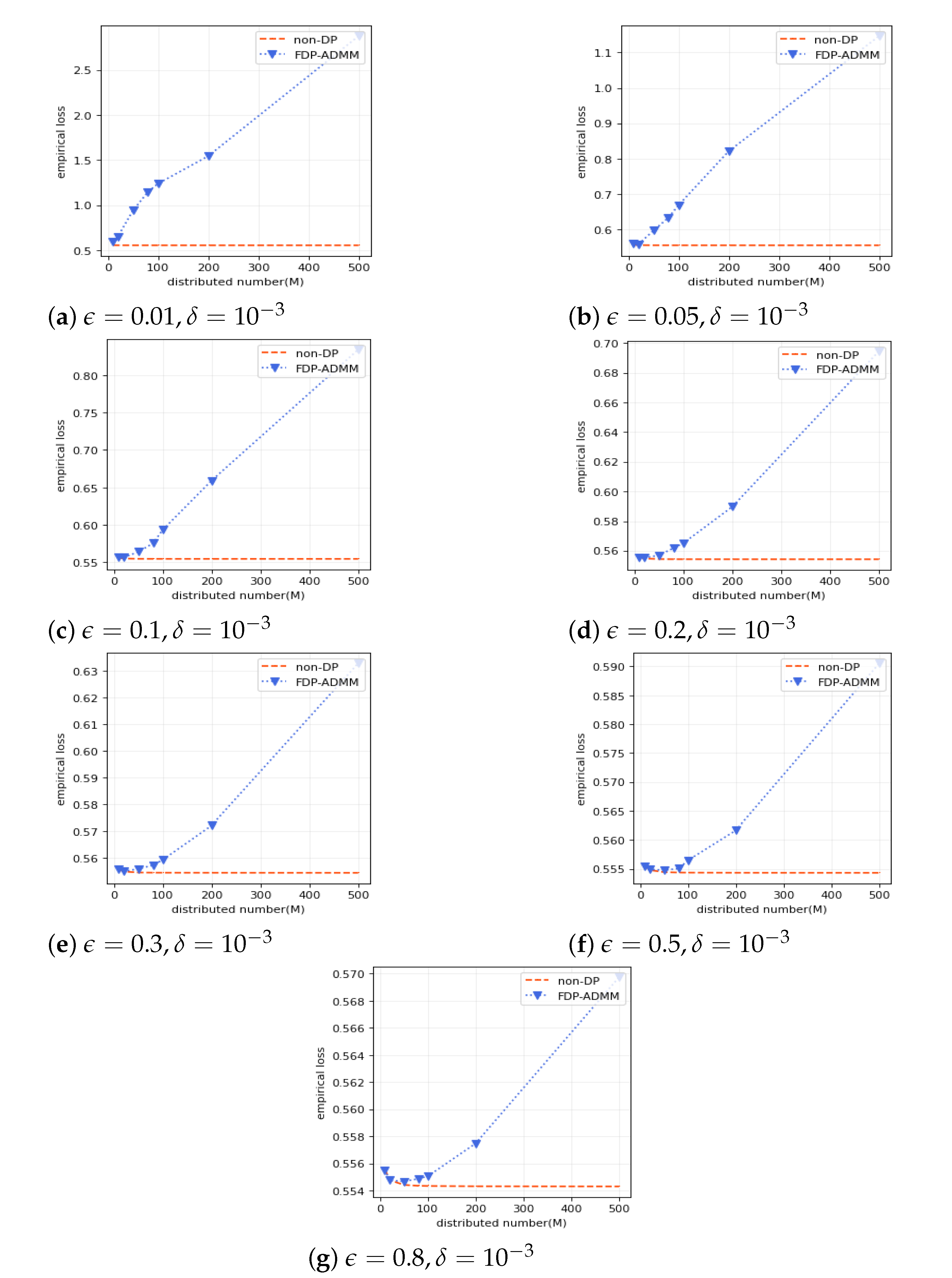
Second, we study the training performance (empirical loss) v.s. different number of distributed data sources under different levels of privacy protection when τ = 0.5 . See Figure 1. Figure 1 shows that the accuracy of our training model will be reduced if more local machines are used. Since the number of agents is larger the smaller the size of the local dataset is, more noise should be added to guarantee the same level of differential privacy. Thus, it results in reducing the performance of the trained model. This is consistent with Theorem 1 that the standard deviation of noises is scaled by 1 / m i . From another perspective, when more local machines participate, a weaker privacy protection can obtain a higher estimation accuracy.
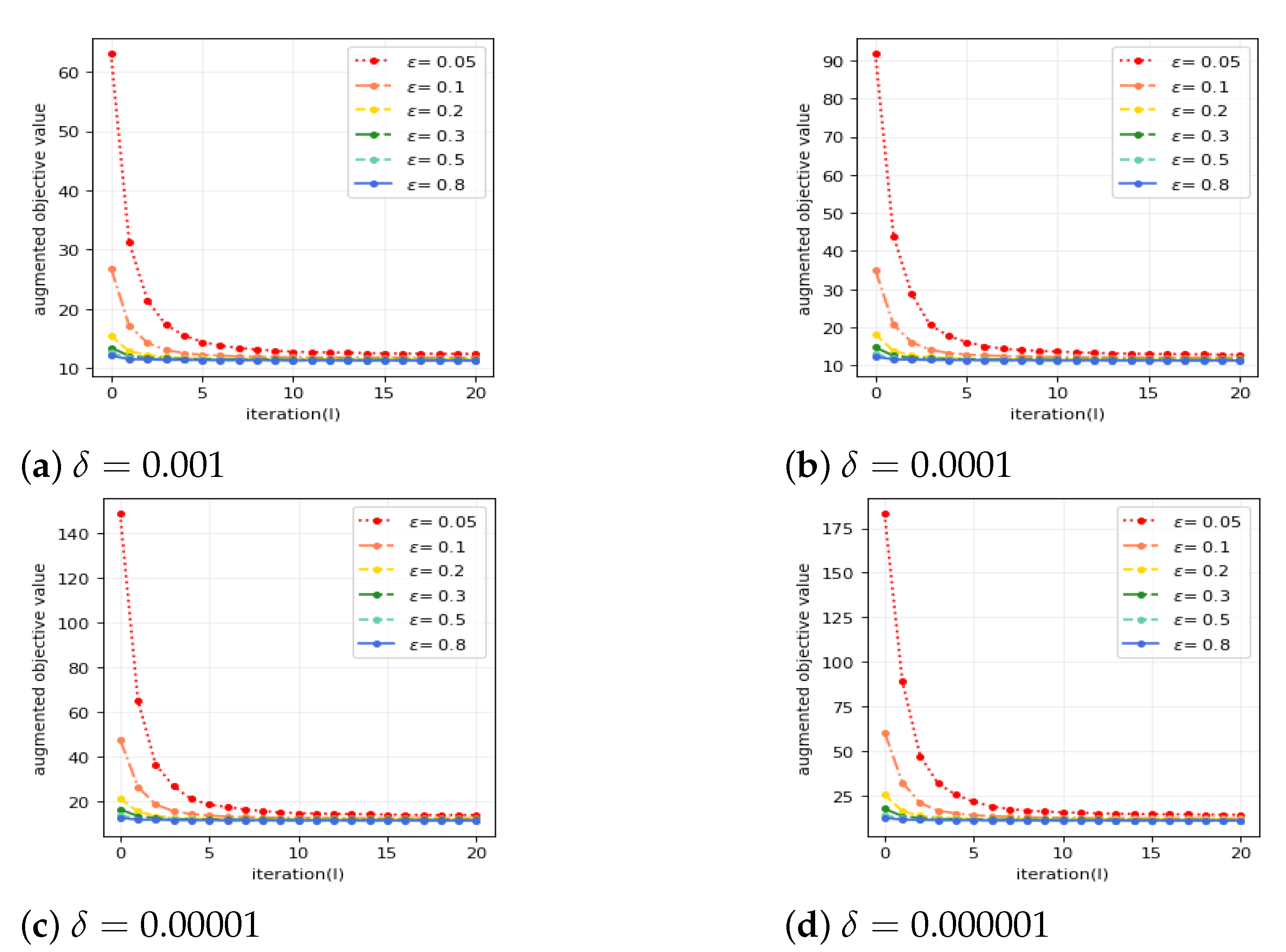
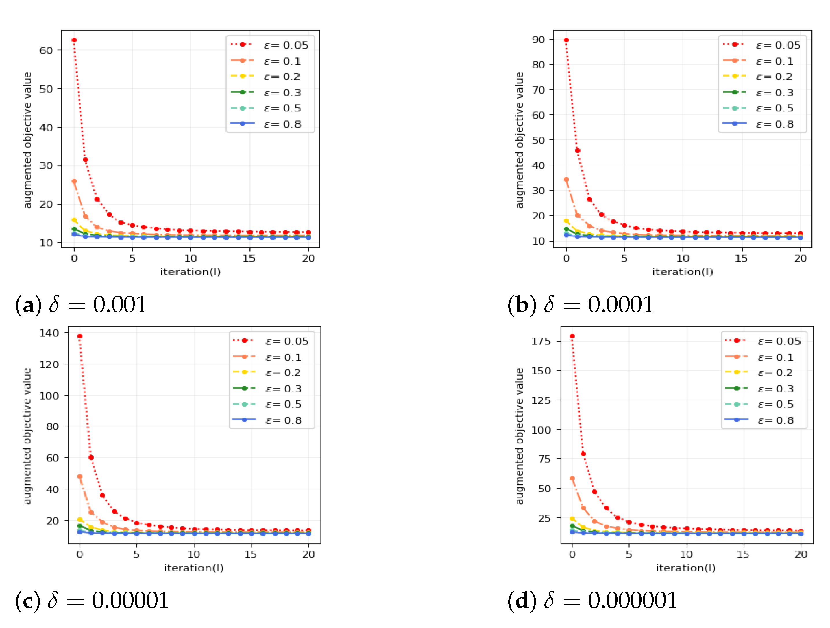
Third, we illustrate the convergence of the FDP-ADMM algorithm by demonstrating how the augmented objective value converges for different values of ϵ and δ . See Figure 2. Figure 2 shows our algorithm with larger ϵ and δ (which implies the weaker privacy protection) has better convergence. This result is consistent with Theorem 2.
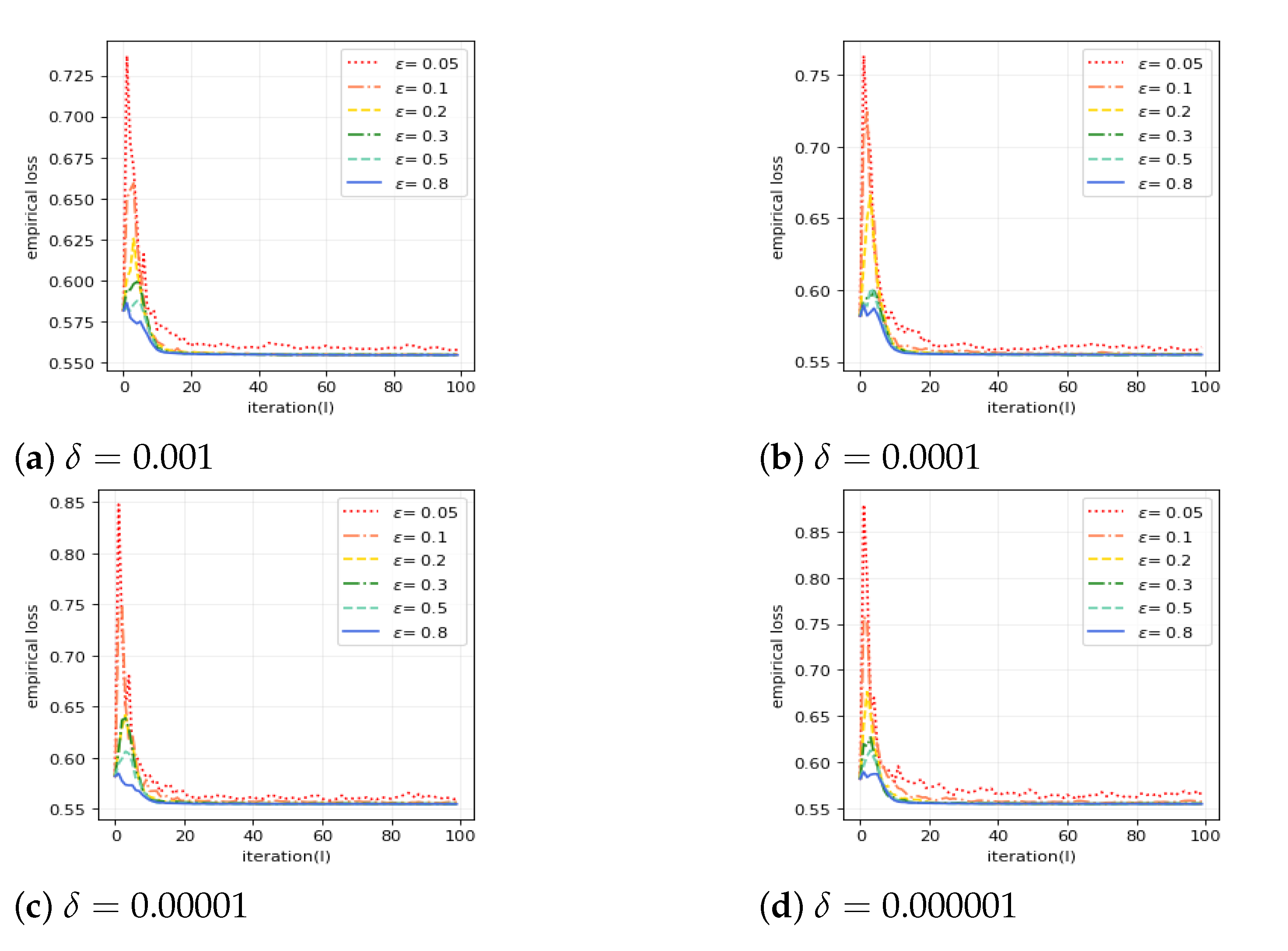
Finally, we evaluate the performance of FDP-ADMM by empirical loss for different levels of privacy protection. See Figure 3. Figure 3 shows our approach has fast convergence property for all privacy policies. In addition, all results we obtained show the privacy–utility trade-off of our FDP-ADMM: better utility is achieved when privacy leakage increases.

5.2. L2-Regularized Quantile Regression

We obtain the FDP-ADMM steps for l 2 -norm quantile regression as follows:
w i l = 1 m i j = 1 m i A i , j T ( τ I { y i , j A i , j w ˜ i l 1 0 } ) λ M w ˜ i l 1 + γ i l 1 + ρ w l 1 + w ˜ i l 1 / η i l ρ + 1 / η i l 1 , w ˜ i l = w i l + N 0 , σ i , l 2 I K , w l = 1 M i = 1 M w ˜ i l 1 M i = 1 M γ i l 1 / ρ , γ i l = γ i l 1 ρ w ˜ i l w l .
Similar to the setting of Section 5.1, we present results in Table 4, Table 5 and Table 6 and Figure 4, Figure 5 and Figure 6. We also obtain the same conclusion as in Section 5.1.

6. Conclusions

In the paper, we proposed an ADMM-based differential privacy learning algorithm on penalized quantile regression for functional data: FDP-ADMM. We first transform functional quantile regression into an ordinary linear regression model by functional principal analysis, and then design the FDP-ADMM algorithm by an approximate augmented Lagrange function, ADMM algorithm, and Gaussian mechanism with time-varying variance. The FDP-ADMM is a noise-resilient, convergent, and computationally effective distributed learning algorithm, even if for high privacy guarantee. Lastly, we obtain the estimation of coefficient function with privacy protection for functional quantile regression distributed model by the Karhunen and Loève expression. We also derived the privacy guarantee and theoretical convergence by the objective value and the constraint violation. The evaluations on simulation datasets have demonstrated the effectiveness of the FDP-ADMM algorithm, even if under high privacy protection, and have shown its privacy–utility trade-off: larger ϵ and larger δ , indicating weaker privacy guarantee, results in better utility.

Author Contributions

Conceptualization, X.Z.; methodology, Y.X.; validation, X.Z. and Y.X.; investigation, X.Z.; writing—original draft preparation, Y.X.; writing—review and editing, X.Z. and Y.X.; supervision, X.Z. All authors have read and agreed to the published version of the manuscript.

Funding

This work was funded by the Chinese National Social Science Fund (19BTJ034), the National Natural Science Foundation of China (12171242, 11971235, 12071220), and the Postgraduate Research and Practice Innovation Program of Jiangsu Province (KYCX21_1940).

Institutional Review Board Statement

Not applicable.

Informed Consent Statement

Not applicable.

Data Availability Statement

Not applicable.

Conflicts of Interest

The authors declare no conflict of interest.

Appendix A

In the Appendix, we give the proofs of Lemma 2 and Theorems 1 and 2.

Appendix A.1. Proof of Lemma 2

Proof
First, we have that L ^ ρ , i w i , w ˜ i l 1 , w l 1 , γ i l 1 is convex because it is a quadratic function of w i . Thus, we have a closed-form solution:
w i , A i l = ρ + 1 / η i l 1 j = 1 m i 1 m i w ˜ i l 1 , A i λ M P w ˜ i l 1 + γ i l 1 + ρ w l 1 + w ˜ i l 1 η i l , w i , A i l = ρ + 1 / η i l 1 j = 1 m i 1 m i i w ˜ i l 1 , A i λ M P w ˜ i l 1 + γ i l 1 + ρ w l 1 + w ˜ i l 1 η i l .
Then, the l 2 -norm sensitivity of primal variable w i l is:
max A i , A i w i , A i l w i , A i l 2 = max A i , A i w ˜ i l 1 , A i w ˜ i l 1 , A i m i ρ + 1 / η i l 2 ( · ) 2 m i ρ + 1 / η i l .
So, Lemma 2 holds. ☐

Appendix A.2. Proof of Theorem 1

Proof
In our quantile loss, we have a subgradient of ρ τ ( u ) , ρ τ ( u ) = τ I { u 0 } , which is bounded. Based on A i j 2 , uniformly bounded, we have the subgradient of ρ τ ( y i j A i j w ) with regard to w, bounded. The privacy loss from w ˜ i l is calculated as:
ln Pr w ˜ i l A i Pr w ˜ i l A i = ln Pr w ˜ i l ( h ) A i Pr w ˜ i l ( h ) A i = ln Pr ξ i l ( h ) Pr ξ i l , ( h ) ,
where ξ i l ( h ) and ξ i l ( h ) are the h-entry of ξ i l and ξ i l , and are sampled from N 0 , σ i , l 2 . The numerator in the ratio above describes the probability of seeing w ˜ i l when the database is A i , the denominator corresponds the probability of seeing this same value when the database is A i . This leads to:
ln Pr w ˜ i l A i Pr w ˜ i l A i = 1 2 σ i , l 2 ξ i l ( h ) 2 ξ i l , ( h ) 2 = 1 2 σ i , l 2 ξ i l ( h ) 2 ξ i l ( h ) + w i , A i l ( h ) w i , A i l ( h ) 2 = 1 2 σ i , l 2 2 ξ i l ( h ) w i , A i l ( h ) w i , A i l ( h ) + w i , A i l ( h ) w i , A i l ( h ) 2 .
Since ( · ) c 1 , according to Lemma 2, we have:
w i , A i l ( h ) w i , A i l ( h ) < w i , A i l w i , A i l 2 c 1 / m i ρ + 1 / η i l .
Thus, by letting σ i , l = 2 c 1 2 ln ( 1.25 / δ ) / m i ϵ ρ + 1 / η i l , we have:
ln Pr w ˜ i l A i Pr w ˜ i l A i ξ i l ( h ) m i ρ + 1 / η i l + c 1 4 ln ( 1.25 / δ ) c 1 / ϵ 2 .
When ξ i l ( h ) 4 ln ( 1.25 / δ ) c 1 / ϵ c 1 / ϵ m i ρ + 1 / η i l , ln Pr w ˜ i l A i / Pr w ˜ i l A i is bounded by ϵ . Next, we need to prove that
Pr ξ i l ( h ) > 4 ln ( 1.25 / δ ) c 1 / ϵ c 1 / ϵ m i ρ + 1 / η i l δ ,
which requires Pr ξ i l ( h ) > 4 ln ( 1.25 / δ ) c 1 / ϵ c 1 / ϵ m i ρ + 1 / η i l δ / 2 . According to the tail bound of normal distribution N 0 , σ i , l 2 , we have
Pr ξ i l ( h ) > r σ i , l r 2 π e r 2 / 2 σ i , l 2 .
By letting r = 4 ln ( 1.25 / δ ) c 1 / ϵ c 1 / ϵ m i ρ + 1 / η i l in the above inequality, we have:
Pr ξ i l ( h ) > 4 ln ( 1.25 / δ ) c 1 / ϵ c 1 m i ρ + 1 / η i l 2 2 ln ( 1.25 / δ ) ( 4 ln ( 1.25 / δ ) ϵ ) 2 π exp ( 4 ln ( 1.25 / δ ) ϵ ) 2 8 ln ( 1.25 / δ ) .
When δ is small ( 0.01 ) and ϵ 1 , we have:
2 2 ln ( 1.25 / δ ) ( 4 ln ( 1.25 / δ ) ϵ ) 2 π < 1 2 π
and
( 4 ln ( 1.25 / δ ) ϵ ) 2 8 ln ( 1.25 / δ ) < ln 2 π δ 2 .
As a result, we have:
Pr ξ i l ( h ) > 4 ln ( 1.25 / δ ) c 1 / ϵ c 1 m i ρ + 1 / η i l < δ 2 .
So far, we have proved that Pr ξ i l ( h ) > 4 ln ( 1.25 / δ ) c 1 / ϵ c 1 / ϵ m i ρ + 1 / η i l δ / 2 ; thus, we can prove that Pr ξ i l ( h ) > 4 ln ( 1.25 / δ ) c 1 / ϵ c 1 / ϵ m i ρ + 1 / η i l δ . Define:
D 1 = ξ i l ( h ) : ξ i l ( h ) 4 ln ( 1.25 / δ ) c 1 / ϵ c 1 m i ρ + 1 / η i l , D 2 = ξ i l ( h ) : ξ i l ( h ) > 4 ln ( 1.25 / δ ) c 1 / ϵ c 1 m i ρ + 1 / η i l .
Therefore, we obtain:
Pr w ˜ i l A i = Pr w i , A i l ( h ) + ξ i l ( h ) : ξ i l ( h ) D 1 + Pr w i , A i l ( h ) + ξ i l ( h ) : ξ i l ( h ) D 2 < e ϵ · Pr w ˜ i l A i + δ ,
which proves that each iteration of DP-ADMM guarantees ( ϵ , δ ) -differential privacy. ☐

Appendix A.3. Proof of Theorem 2

Proof
According to the convexity of f i ( · ) , the monotonicity of the operator F ( · ) , and applying Lemma 3, we have:
i = 1 M f i w ¯ i L f i w i + u ¯ i L u i F u ¯ i L = i = 1 M f i w ¯ i L f i w i + γ ¯ i L , w ¯ i L w i + γ ¯ i L , w ¯ L w + γ ¯ i L γ i , w ¯ i L w ¯ L 1 L l = 1 L i = 1 M f i w ˜ i l 1 f i w i + u i l u i F u i l = 1 L l = 1 L i = 1 M f i w ˜ i l 1 f i w i + γ i l , w ˜ i l w i + γ i l , w l w + γ i l γ i , w ˜ i l w l i = 1 M 1 L l = 1 L η i l 2 f i w ˜ i l ρ + 1 / η i l ξ i l 2 ρ + 1 / η i l ξ i l , w i w ˜ i l 1 + 1 L i = 1 M 1 2 η i L w i w ˜ i 0 2 + ρ 2 w i w 0 2 + 1 2 ρ γ i γ i 0 2 .
Let w i , w be the optimal solution w i * , w * in the above inequality. We obtain:
i = 1 M f i w ¯ i L f i w i * + γ ¯ i L , w ¯ i L w i * + γ ¯ i L , w ¯ L w * + γ ¯ i L γ i , w ¯ i L w ¯ L i = 1 M 1 L l = 1 L η i l 2 f i w ˜ i l 1 ρ + 1 / η i l ξ i l 2 i = 1 M 1 L l = 1 L ρ + 1 / η i l ξ i l , w i * w ˜ i l 1 + 1 L i = 1 M c w 2 2 η i L + M L ρ 2 c w 2 + 1 L i = 1 M 1 2 ρ γ i γ i 0 2 .
The above inequality holds for all γ i ; thus, it also holds for γ i γ i : γ i g . By letting γ i be the optimal solution, we have the maximum of the left side of the above inequality:
max γ i : γ i g i = 1 M f i w ¯ i L f i w i * + γ ¯ i L , w ¯ i L w i * + γ ¯ i L , w ¯ L w * + γ ¯ i L γ i , w ¯ i L w ¯ L = max γ i : γ i g i = 1 M f i w ¯ i L f i w i γ i w ¯ i L w ¯ L = i = 1 M f i w ¯ i L f i w i max γ i : γ i g γ i w ¯ i L w ¯ L = i = 1 M f i w ¯ i L f i w i + g w ¯ i L w ¯ L ;
In addition, we also obtain the maximum of the right side as:
i = 1 M 1 L l = 1 L η i l 2 f i w ˜ i l 1 ρ + 1 / η i l ξ i l 2 i = 1 l 1 L l = 1 L ρ + 1 / η i l ξ i l , w i * w ˜ i l 1 + 1 L i = 1 M c w 2 2 η i L + ρ M 2 L c w 2 + max γ i : γ i g 1 L i = 1 M 1 2 ρ γ i γ i 0 2 = i = 1 M 1 L l = 1 L η i l 2 f i w ˜ i l 1 ρ + 1 / η i l ξ i l 2 i = 1 M 1 L l = 1 L ρ + 1 / η i l ξ i l , w i * w ˜ i l 1 + 1 L i = 1 M c w 2 2 η i L + ρ M 2 L c w 2 + M L g 2 2 ρ .
Thus, we obtain:
i = 1 M f i w ¯ i L f i w i + g w ¯ i L w ¯ L i = 1 M 1 L l = 1 L η i l 2 f i w ˜ i l 1 ρ + 1 / η i l ξ i l 2 i = 1 M 1 L l = 1 L ρ + 1 / η i l ξ i l , w i * w ˜ i l 1 + 1 L i = 1 M c w 2 2 η i L + ρ M 2 L c w 2 + M L g 2 2 ρ .
Since ( · ) c 1 and R ( · ) c 2 , we have:
E f i w ˜ i l 1 ρ + 1 / η i l ξ i l 2 = c 1 + λ c 2 / M 2 + 8 p c 1 2 ln ( 1.25 / δ ) / m i 2 ϵ 2 .
With E ξ i l , w i * w ˜ i l 1 = 0 and η i l = c w 2 l c 1 + λ c 2 / M 2 + 16 l p c 1 2 ln ( 1.25 / δ ) / m i 2 ϵ 2 1 2 , by taking expectation of the previous inequality (A1), we obtain:
E i = 1 M f i w ¯ i L f i w i * + g w ¯ i L w ¯ L i = 1 M 1 L l = 1 L E η i l 2 f i w ˜ i l 1 ρ + 1 / η i l ξ i l 2 i = 1 M 1 L l = 1 L ρ + 1 / η i l E ξ i l , w i * w ˜ i l 1 + 1 L i = 1 M c w 2 2 η i L + ρ M 2 L c w 2 + M L g 2 2 ρ ,
which leads to
E i = 1 n f i w ¯ i L f i w i * + g w ¯ i L w ¯ L = i = 1 M 1 L l = 1 L c w 2 2 l c 1 + λ c 2 / M 2 + 8 p c 1 2 ln ( 1.25 / δ ) m i 2 ϵ 2 + i = 1 M 1 L l = 1 L c w 2 L 2 c 1 + λ c 2 / M 2 + 8 p c 1 2 ln ( 1.25 / δ ) m i 2 ϵ 2 + M ρ 2 t c w 2 + M g 2 2 ρ T = i = 1 M c w 2 2 L c 1 + λ c 2 / M 2 + 8 p c 1 2 ln ( 1.25 / δ ) m i 2 ϵ 2 l = 1 L 1 l + 2 L + M ρ 2 L c w 2 + M g 2 2 ρ L i = 1 M 2 c w L c 1 + λ c 2 / M 2 + 8 p c 1 2 ln ( 1.25 / δ ) m i 2 ϵ 2 + M ρ c w 2 + g 2 / ρ 2 L .
Thus, we complete the proof of Theorem 2. ☐

References

  1. Dwork, C.; Kenthapadi, K.; McSherry, F.; Mironov, I.; Naor, M. Our Data, Ourselves: Privacy Via Distributed Noise Generation. In Proceedings of the Advances in Cryptology—EUROCRYPT 2006, St. Petersburg, Russia, 28 May–1 June 2006; Springer: Berlin/Heidelberg, Germany, 2006; Volume 4004, pp. 486–503. [Google Scholar]
  2. Dwork, C.; McSherry, F.; Nissim, K.; Smith, A. Calibrating Noise to Sensitivity in Private Data Analysis. In Theory of Cryptography; Springer: Berlin/Heidelberg, Germany, 2006; Volume 3876, pp. 265–284. [Google Scholar]
  3. Dwork, C.; Rothblum, G.N.; Vadhan, S. Boosting and Differential Privacy; IEEE Computer Society: Los Alamitos, CA, USA, 2010. [Google Scholar]
  4. Dwork, C.; Roth, A. The algorithmic foundations of differential privacy. Found. Trends® Theor. Comput. Sci. 2014, 9, 211–407. [Google Scholar] [CrossRef]
  5. Dwork, C.; Smith, A.; Steinke, T.; Ullman, J.; Vadhan, S. Robust Traceability from Trace Amounts. In Proceedings of the 2015 IEEE 56th Annual Symposium on Foundations of Computer Science, Berkeley, CA, USA, 17–20 October 2015; pp. 650–669. [Google Scholar]
  6. Abadi, M.; Chu, A.; Goodfellow, I.; McMahan, H.B.; Mironov, I.; Talwar, K.; Zhang, L. Deep Learning with Differential Privacy. In Proceedings of the 2016 ACM SIGSAC Conference on Computer and Communications Security, Vienna, Austria, 24–28 October 2016; Association for Computing Machinery: New York, NY, USA, 2016; pp. 308–318. [Google Scholar]
  7. Differential Privacy Team. Learning with Privacy at Scale. 2017. Available online: https://machinelearning.apple.com/research/learning-with-privacy-at-scale (accessed on 1 February 2022).
  8. Ding, B.; Kulkarni, J.; Yekhanin, S. Collecting Telemetry Data Privately. In Proceedings of the Advances in Neural Information Processing Systems 30 (NIPS 2017), Long Beach, CA, USA, 4–9 December 2017; Volume 30, pp. 3571–3580. [Google Scholar]
  9. Erlingsson, U.; Korolova, A.; Pihur, V. RAPPOR: Randomized Aggregatable Privacy-Preserving Ordinal Response. In Proceedings of the 2014 ACM SIGSAC Conference on Computer and Communications Security, Scottsdale, AZ, USA, 3–7 November 2014; Association for Computing Machinery: New York, NY, USA, 2014; pp. 1054–1067. [Google Scholar]
  10. Wang, J.; Kolar, M.; Srebro, N.; Zhang, T. Efficient Distributed Learning with Sparsity. In Proceedings of the 34th International Conference on Machine Learning, Sydney, Australia, 6–11 August 2017; Volume 70, pp. 3636–3645. [Google Scholar]
  11. He, Y.; Zhou, Y.; Feng, Y. Distributed Feature Selection for High-dimensional Additive Models. arXiv 2022, arXiv:2205.07932. [Google Scholar]
  12. Jordan, M.I.; Lee, J.D.; Yang, Y. Communication-Efficient Distributed Statistical Inference. J. Am. Stat. Assoc. 2019, 114, 668–681. [Google Scholar] [CrossRef]
  13. Hu, A.; Jiao, Y.; Liu, Y.; Shi, Y.; Wu, Y. Distributed quantile regression for massive heterogeneous data. Neurocomputing 2021, 448, 249–262. [Google Scholar] [CrossRef]
  14. Nedic, A.; Olshevsky, A.O.A.; Tsitsiklis, J.N. Distributed subgradient methods and quantization effects. In Proceedings of the 47th IEEE Conference on Decision and Control, Cancun, Mexico, 9–11 December 2008; Institute of Electrical and Electronics Engineers Inc.: Piscataway, NJ, USA, 2008; pp. 4177–4184. [Google Scholar]
  15. Nedic, A.; Ozdaglar, A. Distributed Subgradient Methods for Multi-Agent Optimization. IEEE Trans. Autom. Control. 2009, 54, 48–61. [Google Scholar] [CrossRef]
  16. Boyd, S.; Parikh, N.; Chu, E.; Peleato, B.; Eckstein, J. Distributed Optimization and Statistical Learning via the Alternating Direction Method of Multipliers. Found. Trends® Mach. Learn. 2011, 3, 1–122. [Google Scholar]
  17. Ling, Q.; Ribeiro, A. Decentralized linearized alternating direction method of multipliers. In Proceedings of the 2014 IEEE International Conference on Acoustics, Speech and Signal Processing (ICASSP), Florence, Italy, 4–9 May 2014; pp. 5447–5451. [Google Scholar]
  18. Shi, W.; Ling, Q.; Yuan, K.; Wu, G.; Yin, W. On the Linear Convergence of the ADMM in Decentralized Consensus Optimization. IEEE Trans. Signal Process. 2014, 62, 1750–1761. [Google Scholar] [CrossRef]
  19. Zhang, R.; Kwok, J. Asynchronous distributed ADMM for consensus optimization. In Proceedings of the 31st International Conference on Machine Learning, Beijing, China, 21–26 June 2014; Volume 5, pp. 3689–3697. [Google Scholar]
  20. Bianchi, P.; Hachem, W.; Iutzeler, F. A stochastic primal-dual algorithm for distributed asynchronous composite optimization. In Proceedings of the 2014 IEEE Global Conference on Signal and Information Processing (GlobalSIP), Atlanta, GA, USA, 3–5 December 2014; pp. 732–736. [Google Scholar]
  21. Wei, E.; Ozdaglar, A. Distributed Alternating Direction Method of Multipliers. In Proceedings of the 2012 IEEE 51st IEEE Conference on Decision and Control (CDC), Maui, HI, USA, 10–13 December 2012; pp. 5445–5450. [Google Scholar]
  22. Shokri, R.; Stronati, M.; Song, C.; Shmatikov, V. Membership Inference Attacks Against Machine Learning Models. In Proceedings of the 2017 IEEE Symposium on Security and Privacy (SP), San Jose, CA, USA, 22–24 May 2017; pp. 3–18. [Google Scholar]
  23. Fredrikson, M.; Jha, S.; Ristenpart, T. Model Inversion Attacks that Exploit Confidence Information and Basic Countermeasures. In Proceedings of the 22nd ACM Conference on Computer and Communications Security, Denver, CO, USA, 12–16 October 2015; pp. 1322–1333. [Google Scholar]
  24. Zhang, T.; Zhu, Q. Dynamic Differential Privacy for ADMM-Based Distributed Classification Learning. IEEE Trans. Inf. Forensics Secur. 2017, 12, 172–187. [Google Scholar] [CrossRef]
  25. Guo, Y.; Gong, Y. Practical Collaborative Learning for Crowdsensing in the Internet of Things with Differential Privacy. In Proceedings of the 2018 IEEE Conference on Communications and Network Security (CNS), Beijing, China, 30 May–1 June 2018; pp. 1–9. [Google Scholar]
  26. Ding, J.; Errapotu, S.M.; Zhang, H.; Gong, Y.; Pan, M.; Han, Z. Stochastic ADMM Based Distributed Machine Learning with Differential Privacy. Secur. Priv. Commun. Netw. 2019, 304, 257–277. [Google Scholar]
  27. Ferraty, F.; Vieu, P. Nonparametric Functional Data Analysis; Springer: New York, NY, USA, 2006. [Google Scholar]
  28. Ramsay, J.O.; Silverman, B.W. Functional Data Analysis, 2nd ed.; Springer: New York, NY, USA, 2005. [Google Scholar]
  29. Zhang, J.T. Analysis of Variance for Functional Data; Chapman and Hall/CRC: New York, NY, USA, 2013. [Google Scholar]
  30. Ramsay, J.O.; Silverman, B.W. Applied Functional Data Analysis: Methods and Case Studies; Springer: New York, NY, USA, 2002. [Google Scholar]
  31. Ramsay, J.O.; Dalzell, C.J. Some Tools for Functional Data Analysis. J. R. Stat. Soc. Ser. Methodol. 1991, 53, 539–561. [Google Scholar] [CrossRef]
  32. Tang, Q.; Kong, L. Quantile regression in functional linear semiparametric model. Statistics 2017, 51, 1342–1358. [Google Scholar]
  33. Lu, Y.; Du, J.; Sun, Z. Functional partially linear quantile regression model. Metrika 2014, 77, 317–332. [Google Scholar] [CrossRef]
  34. Auton, T. Applied Functional Data Analysis: Methods and Case Studies. J. R. Stat. Soc. Ser. Stat. Soc. 2004, 167, 378–379. [Google Scholar] [CrossRef]
  35. Hall, P.; Horowitz, J.L. Methodology and convergence rates for functional linear regression. Ann. Stat. 2007, 35, 70–91. [Google Scholar] [CrossRef]
  36. Karhunen, K. Zur Spektraltheorie stochastischer Prozesse. Ann. Acad. Sci. Fenn. 1946, 1, 7. [Google Scholar]
  37. Tibshirani, R. Regression shrinkage and selection via the lasso: A retrospective. J. R. Stat. Soc. Ser. Stat. Methodol. 2011, 73, 273–282. [Google Scholar] [CrossRef]
  38. Zou, H.; Hastie, T. Regularization and variable selection via the Elastic Net. J. R. Stat. Soc. Ser. B 2005, 67, 301–320. [Google Scholar] [CrossRef]
  39. Zhang, C. Nearly unbiased variable selection under minimax concave penalty. Ann. Stat. 2010, 38. [Google Scholar] [CrossRef]
  40. Fan, J.; Li, R. Variable Selection via Nonconcave Penalized Likelihood and its Oracle Properties. J. Am. Stat. Assoc. 2001, 96, 1348–1360. [Google Scholar] [CrossRef]
  41. Glowinski, R.; Marroco, A. Sur l’approximation, par éléments finis d’ordre un, et la résolution, par pénalisation-dualité d’une classe de problèmes de Dirichlet non linéaires. ESAIM Math. Model. Numer. Anal. 1975, 9, 41–76. [Google Scholar] [CrossRef]
  42. Gabay, D.; Mercier, B. A dual algorithm for the solution of nonlinear variational problems via finite element approximation. Comput. Math. Appl. 1976, 2, 17–40. [Google Scholar] [CrossRef]
  43. Huang, Z.; Gong, Y. Differentially Private ADMM for Convex Distributed Learning: Improved Accuracy via Multi-Step Approximation. arXiv 2020, arXiv:2005.07890. [Google Scholar]
  44. Deng, W.; Yin, W. On the Global and Linear Convergence of the Generalized Alternating Direction Method of Multipliers. J. Sci. Comput. 2016, 66, 889–916. [Google Scholar] [CrossRef]
  45. Wang, H.; Banerjee, A. Bregman Alternating Direction Method of Multipliers. Adv. Neural Inf. Process. Syst. 2014, 4, 2816–2824. [Google Scholar]
  46. Hong, M.; Luo, Z. On the Linear Convergence of the Alternating Direction Method of Multipliers. Math. Program. 2017, 162, 165–199. [Google Scholar] [CrossRef]
  47. Eckstein, J.; Bertsekas, D.P. On the Douglas-Rachford splitting method and the proximal point algorithm for maximal monotone operators. Math. Program. 1992, 55, 293–318. [Google Scholar] [CrossRef]
  48. He, B.; Yuan, X. On the O(1/n) Convergence Rate of the Douglas-Rachford Alternating Direction Method. SIAM J. Numer. Anal. 2012, 50, 700–709. [Google Scholar] [CrossRef]
  49. Sun, J.; Zhang, S. A modified alternating direction method for convex quadratically constrained quadratic semidefinite programs. Eur. J. Oper. Res. 2010, 207, 1210–1220. [Google Scholar] [CrossRef]
  50. Zhang, S.; Ang, J.; Sun, J. An alternating direction method for solving convex nonlinear semidefinite programming problems. Optimization 2013, 62, 527–543. [Google Scholar] [CrossRef]
  51. Goldstein, T.; O’Donoghue, B.; Setzer, S.; Baraniuk, R. Fast Alternating Direction Optimization Methods. SIAM J. Imaging Sci. 2014, 7, 1588–1623. [Google Scholar] [CrossRef]
  52. Gabay, D. Chapter IX Applications of the Method of Multipliers to Variational Inequalities. Augment. Lagrangian Methods Appl. Solut. -Bound.-Value Probl. 1983, 15, 299–331. [Google Scholar]
  53. Li, G.; Pong, T. Global Convergence of Splitting Methods for Nonconvex Composite Optimization. SIAM J. Optim. 2015, 25, 2434–2460. [Google Scholar] [CrossRef]
  54. Yu, L.; Lin, N. ADMM for Penalized Quantile Regression in Big Data. Int. Stat. Rev. 2017, 85, 494–518. [Google Scholar] [CrossRef]
  55. Huang, Z.; Hu, R.; Guo, Y.; Chan-Tin, E.; Gong, Y. DP-ADMM: ADMM-Based Distributed Learning With Differential Privacy. IEEE Trans. Inf. Forensics Secur. 2020, 15, 1002–1012. [Google Scholar] [CrossRef]
Figure 1. Impact of the number of distributed data sources on FDP-ADMM for l 1 -regularized quantile regression.
Mathematics 10 02954 g001
Figure 2. Convergence properties of FDP-ADMM via augmented objective value for l 1 -regularized quantile regression with τ = 0.5 .
Mathematics 10 02954 g002
Figure 3. Convergence properties of FDP-ADMM via empirical loss for l 1 -regularized quantile regression τ = 0.5 .
Mathematics 10 02954 g003
Figure 4. Impact of the number of distributed data sources on FDP-ADMM for l 2 -regularized quantile regression.
Mathematics 10 02954 g004
Figure 5. Convergence properties of FDP-ADMM via augmented objective value for l 2 -regularized quantile regression with τ = 0.5 .
Mathematics 10 02954 g005
Figure 6. Convergence properties of FDP-ADMM via empirical loss for l 2 -regularized quantile regression τ = 0.5 .
Mathematics 10 02954 g006
Table 1. MISEs of FDP-ADMM algorithm for l 1 -regularized quantile regression when M = 10 .
M = 10
ϵ δ τ = 0.1 τ = 0.25 τ = 0.5 τ = 0.75 τ = 0.9
0.1 10 6 1.109351.082721.080421.067721.15352
10 5 1.014720.888990.639390.729650.81495
10 4 1.000920.508740.619400.426691.20186
10 3 0.767010.519940.437490.457140.83579
0.2 10 6 0.882930.493520.379030.485731.13445
10 5 0.860120.493980.352140.432330.93748
10 4 0.855130.477090.402590.454890.89320
10 3 0.976300.458290.363650.428390.95078
0.3 10 6 0.759550.407470.371030.438720.99364
10 5 0.806880.405630.387850.438341.16647
10 4 0.824620.436170.370860.426791.08880
10 3 0.882120.430030.362110.431410.88249
0.5 10 6 0.946820.466870.371580.428120.96098
10 5 0.927090.440070.388630.424470.89955
10 4 0.937760.436480.365950.447080.89621
10 3 0.956110.425110.374810.451990.98540
0.8 10 6 0.872320.440240.383080.443780.96025
10 5 0.903690.444780.378630.447280.99718
10 4 0.916700.438550.377690.454730.92953
10 3 0.931210.430900.375370.437510.94244
10.925880.435360.382910.448200.98044
Table 2. MISEs of FDP-ADMM algorithm for l 1 -regularized quantile regression when M = 20 .
M = 20
ϵ δ τ = 0.1 τ = 0.25 τ = 0.5 τ = 0.75 τ = 0 . 9
0.1 10 6 9.142067.578618.632085.999937.25853
10 5 4.913133.390253.845674.725252.98801
10 4 4.075481.994892.157431.737283.75287
10 3 1.198300.928990.899241.387341.72083
0.2 10 6 1.278891.075830.911181.384001.39675
10 5 1.122620.648320.689670.606050.97722
10 4 0.796000.486210.407880.325990.59192
10 3 0.589560.354900.280230.367160.79028
0.3 10 6 0.679980.489550.395350.426770.69698
10 5 0.626560.340880.315100.365010.82977
10 4 0.640470.352140.230910.423890.52364
10 3 0.642560.336830.311040.370060.65798
0.5 10 6 0.480450.379460.283040.381710.60391
10 5 0.586200.355720.326570.354700.53452
10 4 0.604730.320190.295400.359350.61225
10 3 0.554530.354110.319890.369620.61693
0.8 10 6 0.621390.349650.289700.362320.61739
10 5 0.569930.333110.320590.351610.52785
10 4 0.590240.366450.319040.347260.60428
10 3 0.541070.357530.322110.359590.61891
10.571590.363870.344850.367570.60352
Table 3. MISEs of FDP-ADMM algorithm for l 1 -regularized quantile regression when M = 50 .
M = 50
ϵ δ τ = 0.1 τ = 0.25 τ = 0.5 τ = 0.75 τ = 0.9
0.1 10 6 32.6909245.6174118.5795142.8952626.78259
10 5 19.5440418.2804224.9864914.5602423.62843
10 4 9.2574415.3526814.2139516.5115415.62429
10 3 8.480438.026629.361178.5400510.24176
0.2 10 6 7.3083810.650706.654398.118068.28644
10 5 3.281297.682745.461425.372286.88005
10 4 3.691343.302372.536012.689054.13535
10 3 1.235771.463820.893651.122391.55549
0.3 10 6 2.778992.963512.070312.923102.93987
10 5 2.799872.226341.834201.727591.82370
10 4 1.210770.999001.300570.938721.55615
10 3 0.788470.538790.457380.519680.78215
0.5 10 6 0.951850.794080.943530.857461.39231
10 5 0.910100.905030.548370.612160.83725
10 4 0.698610.374400.441300.413320.55033
10 3 0.476770.290990.263890.286540.50744
0.8 10 6 0.438620.425970.285140.418430.57740
10 5 0.698380.321060.244530.336190.55950
10 4 0.519370.396850.226640.280520.42013
10 3 0.466010.261870.206170.247690.38190
10.437150.309220.2299190.293830.45229
Table 4. MISEs of FDP-ADMM algorithm for l 2 -regularized quantile regression when M = 10 .
M = 10
ϵ δ τ = 0.1 τ = 0.25 τ = 0.5 τ = 0.75 τ = 0.9
0.1 10 6 2.892102.753532.469412.547803.81696
10 5 2.925842.272352.094342.273902.86815
10 4 1.374341.528571.635191.011531.76823
10 3 0.994950.950070.903491.124171.11879
0.2 10 6 1.142631.077200.693401.030471.25381
10 5 0.893390.609440.765080.702921.22899
10 4 0.761410.603310.430440.563150.87222
10 3 0.617300.580380.382350.429830.67101
0.3 10 6 0.892910.524950.532380.504710.90524
10 5 0.825940.525620.347340.488370.83485
10 4 0.616220.438490.342530.473890.52728
10 3 0.502650.342560.248520.365760.58658
0.5 10 6 0.506570.357740.331480.360340.61492
10 5 0.623030.317070.259260.331310.56412
10 4 0.441780.329440.278090.275200.56905
10 3 0.554270.313990.229240.275810.53565
0.8 10 6 0.481120.303660.261900.293830.54639
10 5 0.523030.315190.214920.309340.49795
10 4 0.512000.294940.255460.266510.51737
10 3 0.497100.328420.219900.261140.49119
10.474300.279010.208530.269260.49421
Table 5. MISEs of FDP-ADMM algorithm for l 2 -regularized quantile regression when M = 20 .
M = 20
ϵ δ τ = 0.1 τ = 0.25 τ = 0.5 τ = 0.75 τ = 0.9
0.1 10 6 12.098827.537538.994899.2850010.41200
10 5 6.369084.833249.443845.385157.07413
10 4 5.402123.781142.922585.801283.78069
10 3 3.568651.670932.027143.120412.73505
0.2 10 6 2.351282.409282.474913.138112.81266
10 5 2.441511.864172.141901.792861.69856
10 4 1.253331.128281.060311.294331.47163
10 3 1.003800.679440.759940.892211.20207
0.3 10 6 1.447731.215301.829651.162741.67580
10 5 0.923050.842150.986730.874020.83162
10 4 0.611510.500560.627190.752691.11462
10 3 0.794220.432390.468190.439580.65150
0.5 10 6 0.652240.498340.692980.502190.72637
10 5 0.526230.486790.391950.414690.81617
10 4 0.456040.446200.393560.356840.54628
10 3 0.485890.354960.261640.283090.44583
0.8 10 6 0.585540.367760.362100.357510.44102
10 5 0.563100.375120.246210.380690.41426
10 4 0.469340.302160.225640.275540.43864
10 3 0.391100.220990.228960.225800.42480
10.374680.219740.162010.201350.38618
Table 6. MISEs of FDP-ADMM algorithm for l 2 -regularized quantile regression when M = 50 .
M = 50
ϵ δ τ = 0.1 τ = 0.25 τ = 0.5 τ = 0.75 τ = 0.9
0.1 10 6 28.6120840.7221629.5671319.8280022.75443
10 5 24.2935510.6140523.4865525.2893616.24641
10 4 18.6151810.5680915.6312018.8719514.77067
10 3 8.2323611.809486.469548.759017.39285
0.2 10 6 9.216397.3066110.831666.509476.74332
10 5 5.332377.205206.489284.993316.98322
10 4 3.695574.257205.239054.259164.26556
10 3 2.649443.403412.101491.803722.19432
0.3 10 6 3.721355.267654.626682.824332.56538
10 5 3.529953.494323.829022.465282.24935
10 4 2.101022.306791.913622.487652.40823
10 3 1.343451.653471.230161.022931.63715
0.5 10 6 1.766211.917851.388611.419122.15178
10 5 1.148480.918371.254441.123650.96906
10 4 0.825131.111080.790600.870091.03410
10 3 0.630680.473020.417470.480540.59396
0.8 10 6 0.750220.860220.722340.830850.91919
10 5 0.881040.912870.595280.526520.47342
10 4 0.520610.447820.337730.434060.61304
10 3 0.390310.377080.265190.285730.42317
10.310620.187290.137620.166530.31931
Publisher’s Note: MDPI stays neutral with regard to jurisdictional claims in published maps and institutional affiliations.

