Steganography with High Reconstruction Robustness: Hiding of Encrypted Secret Images

Abstract

As one of the important methods to protect information security, steganography can ensure the security of data in the process of information transmission, which has attracted much attention in the information security community. However, many current steganography algorithms are not sufficiently resistant to recent steganalysis algorithms, such as deep learning-based steganalysis algorithms. In this manuscript, a new steganography algorithm, based on residual networks and pixel shuffle, is proposed, which combines image encryption and image hiding, named Resen-Hi-Net, an algorithm that first encrypts a secret image and then hides it in a carrier image to produce a meaningful container image. The proposed Resen-Hi-Net has the advantages of both image encryption and image hiding. The experimental results showed that the proposed Resen-Hi-Net could realize both image encryption and image hiding; the visual container image quality was as high as 40.19 dB on average in PSNR to reduce the possibility of being attacked, and the reconstructed secret image quality was also good enough (34.39 dB on average in PSNR). In addition, the proposed Resen-Hi-Net has a strong ability to resist destructive attacks and various steganographic analyses.

1. Introduction

Encryption and information hiding are the two main measures to ensure information security. Encryption is the transformation of data into disordered ciphertext via cryptographic algorithms. The essence of image encryption is to change the pixel positions or pixel values of an image so that the image becomes visually similar to noise or texture [1,2,3]. To increase the key space and flexibility, some image encryption techniques, such as fractional discrete cosine transform [4,5,6], fractional chaotic systems [7], fractional wavelet transform [8], fractional Fourier transform [9,10], and multi-parameter discrete fractional random transform [11], use fractional-order transformations with additional free parameters as auxiliary keys. However, these encryption models are vulnerable to various cryptographic attacks by eavesdroppers. Unlike encryption, steganography is a technique that hides information in a host to avoid the attention of eavesdroppers. Common hosts include: images [12], audio [13], text [14], video [15], compressed files [16], etc. Among these, images are the most commonly used information carriers due to their strong intuition and comprehensiveness. Image steganography has now become an important branch in the field of information security.

The application of steganography in digital media can be traced back to the 1990s. Bender et al. [17] proposed the earliest image steganography algorithm, which consisted of a digital image steganography algorithm based on the least significant bit (LSB). This algorithm embeds secret information by changing the lowest bits of the pixels. Similar to the LSB algorithm, in the compression domain, the information is considered to be hidden in the lowest bits of the quantized discrete cosine transform (DCT) coefficients, resulting in algorithms, such as Jsteg [18] and F5 [19]. However, these algorithms belong to non-adaptive steganography algorithms that do not consider the texture complexity of the image when embedding secret information. In 2011, Fridrich [20] proposed an image steganography framework by minimizing the embedding of arbitrary additive distortion functions. He used syndrome-trellis codes to improve the security of existing steganographic algorithms and reduce distortion for a given payload. Generally, the above-mentioned steganographic algorithms use manually-designed distortion functions, such as the weighted difference of eigenvectors used in the highly undetectable steGO (Hugo) [21], the cost sum of pixel change differences used in the wavelet obtained weights (WOW) [22] and the sum of relative changes of the wavelet coefficients used in the spatial-domain universal wavelet relative distortion (S-UNIWARD) [23]. It requires a long time of knowledge accumulation and continuous attempts. In addition, the traces in the carrier image resulting from the secret information embedding in traditional steganography algorithms can be easily detected by steganalysis.

With the rise of deep learning, the deep learning-based image steganography algorithm has attracted much attention in the information security community. In 2016, Volkhonskiy et al. [24] proposed the first deep learning-based image steganography algorithm. The algorithm was based on a deep convolutional generative adversarial network (DCGAN), including a generator (G), a discriminator (D), and a steganalyzer (S). G is responsible for generating image samples, D is responsible for determining whether the samples are real or generated samples, and S is responsible for evaluating the security of the container images generated after steganography embedding. Subsequently, more steganography algorithms, based on generative adversarial networks (GAN) [25], were proposed, such as SSGAN [26], ADSL-GAN [27], Hiding GAN [28], etc. [29,30]. These new steganography methods not only reduce human participation, but also effectively enhance the security of steganography. However, there are still some problems, such as instability of network architecture and irreversibility of the GAN network.

The steganography methods based on convolutional neural network (CNN) are different from those based on GAN. They hide secret images based on global feature mapping. Baluja [31] proposed an image steganography model based on an automatic encoder framework, which hides an image of the same size in another image. Rehman et al. [32] proposed an end-to-end training method and trained a pair of encoded and decoded CNNs to hide images into other images. To improve security and reliability, Wang et al. [33] proposed a novel steganographic network based on style transfer (STNet). To further improve the capacity of steganography, Baluja [34] attempted to hide two color images of the same size into one color image. Wang et al. [35] also proposed a high-capacity image steganography that can hide up to four images in a host image by naturally increasing the number of channels in the hidden image branch. Zhu et al. [36] proposed a high-capacity image hiding algorithm based on residual CNN in wavelet domain, which has a maximum capacity of 32 times that of the carrier. However, the high-capacity embedding ratio poses security risks and is more easily detected by recent deep learning-based steganalyses.

Among the evaluation indicators of the above-mentioned steganography algorithms, capacity is an important one. For example, in the literature [34,35,36], the focus has always been on how to improve the image hiding capacity of steganography. However, the increase in capacity comes at the cost of security threats, along with reduced ability to resist steganalysis, cropping, compression, and noise attacks. In [36], the image hiding capacity reached up to 32, but the resistance against some attacks, such as cropping and compression, was unsatisfactory. Therefore, in this paper, we propose a new image hiding model to improve the hiding capacity, while maintaining resistance to various steganalyses and common image manipulation attacks.

In this paper, we propose a new image-hiding convolutional neural Network based on Residual network and pixel Shuffle combined with image Encryption, named Resen-Hi-Net. Resen-Hi-Net basically consists of an encryption module, an image hiding network and a recovery network (i.e., Torch-Net). To reduce the possibility of being attacked, and to increase the difficulty of steganalysis algorithms, the secret image was first encrypted and then hidden in the carrier image, resulting in a visually meaningful container image. To recover the secret image, a Torch-Net was modeled as a recovery network, including a pyramid at the bottom and an inverted pyramid at the top. The hidden information was extracted from the pyramid and the secret image was gradually reconstructed through the layers of the inverted pyramid.

2. Related Work and Evaluation Indexes

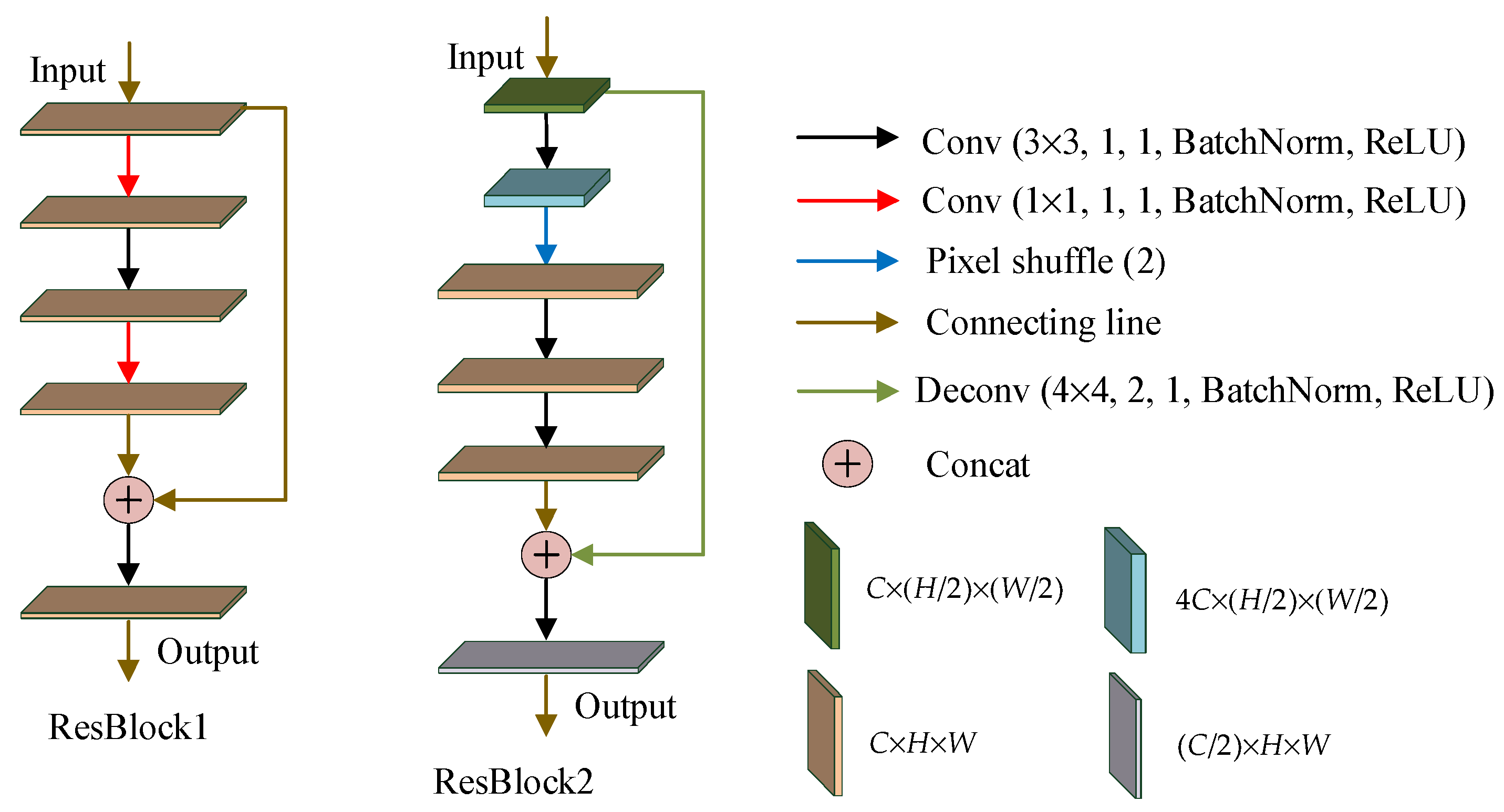
2.1. Residual Convolutional Neural Network (RCNN)

The RCNN, originally proposed by He [37], adds a branch of jump connections, compared to the traditional CNN. The residual network solves the degradation problem of the deep neural network very well [38]. Under the premise of the same number of layers, the convergence speed of the residual network is faster. In the steganography algorithm proposed in this paper, two different ResBlocks were used, as shown in Figure 1. It can be seen from Figure 1 that ResBlock1 was used to deepen the network depth and bring the shallow information into the deeper layer. ResBlock2 amplified the input feature maps and transmitted them to the later layers.

2.2. Pixel Shuffle

Upsampling, in the framework of deep learning, can simply be understood as any technology that can make an image become higher in resolution. In PyTorch, there are four types of upsampling implementations: Pixel shuffle, Upsample, UpsamplingNearest2d, and UpsamplingBilinear2d. The latter three types are each used to upsample the input tensor by padding zeros and to enlarge the size of the input feature maps. These adjacent pixel filling algorithms mainly consider the space factor, but not the channel factor. Artificial modification traces are obvious and image restoration effect is poor. Pixel shuffler fills pixels with channel dimensional information, which can achieve ultra-high resolution and generate more realistic and perfect images [39].

2.3. Image Encryption Algorithm

Wu et al. [40] proposed a highly nonlinear image encryption approach that can resist common attacks, such as differential attack. This approach combines antagonistic neural cryptography (ANC) and SHA-256 controlled chaotic systems. In the image encryption phase in Resen-Hi-Net, the secret image is encrypted with the aid of this approach and then embedded in a carrier.

2.4. Evaluation Indexes

Mean square error (MSE), peak signal-to-noise ratio (PSNR) [41], mean structural similarity (MSSIM) [42], and mean absolute pixel error (APE) [36] were used to evaluate the quality and difference of images. In this paper, they were used to evaluate the differences between carriers and containers, secret images and reconstructed secret images. For color images, a metric was the average of three metrics over the channels R, G, and B.

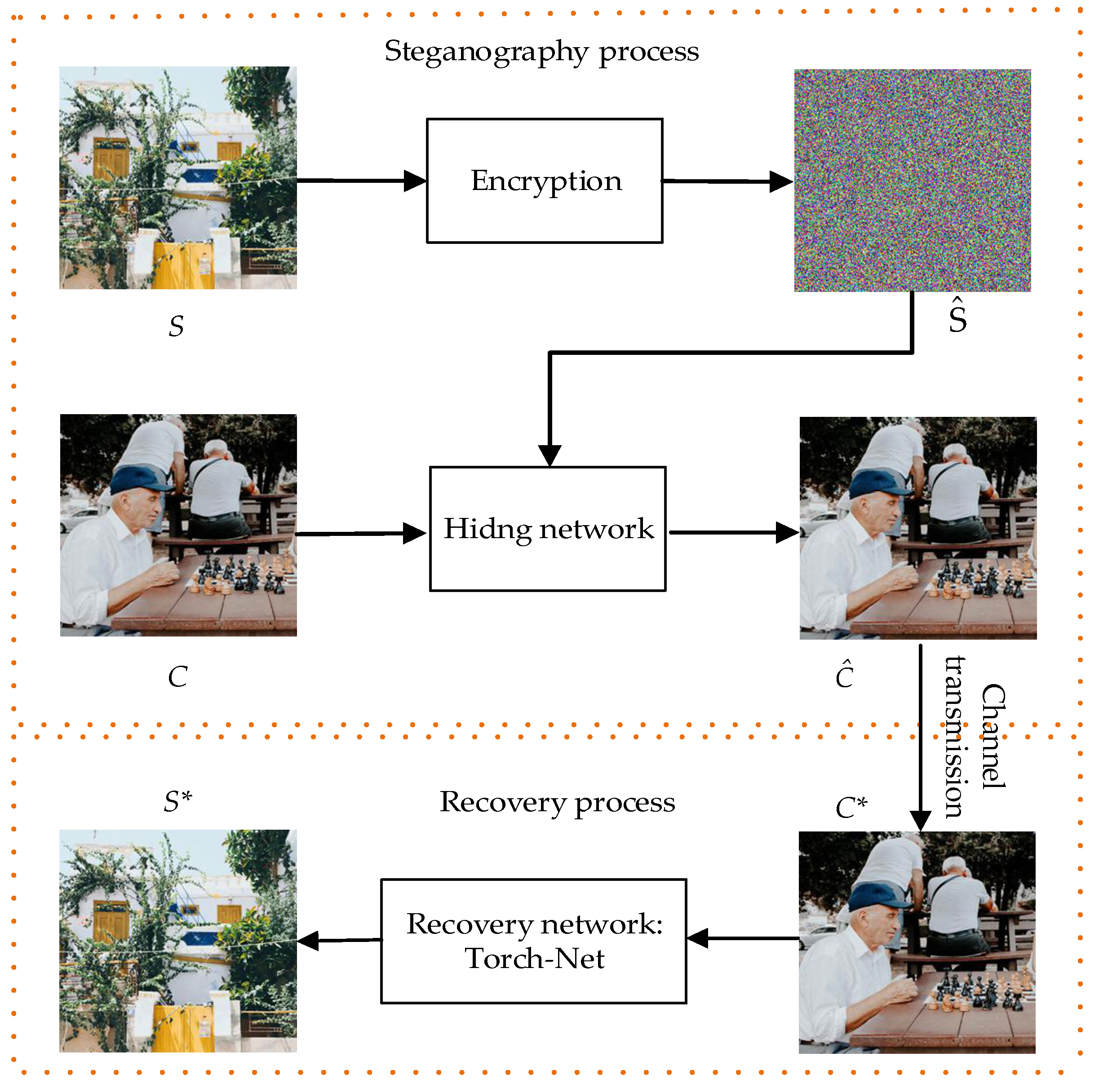
3. The Proposed Resen-Hi-Net

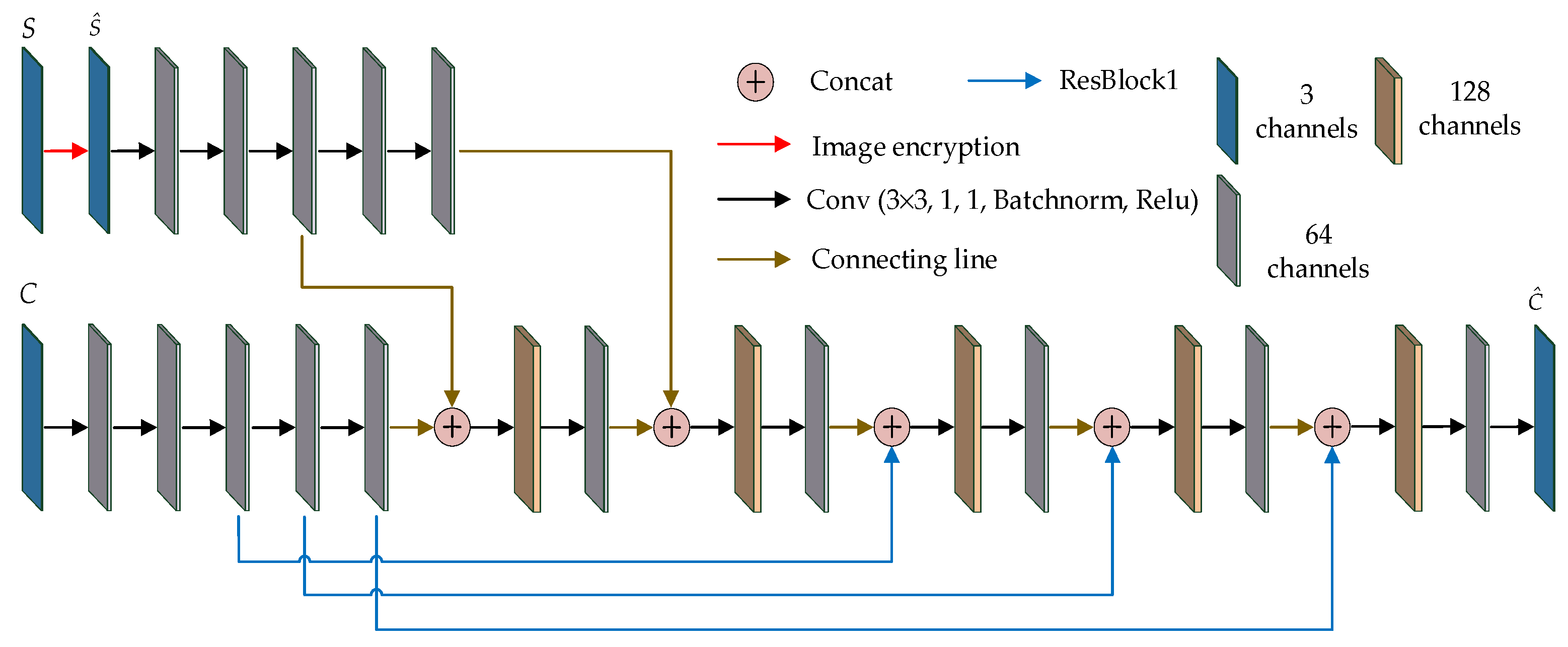
The proposed Resen-Hi-Net steganography network is shown in Figure 2. First, the secret image was encrypted using the algorithm in Section 2.3, and the encrypted result was embedded into the carrier image in the hiding network, resulting in the container image. After channel transmission, at the receiving end, the container containing the secret image was the input to the recovery network (Torch-Net), and, Torch-Net output the reconstructed secret image, as shown in Figure 2, where some notations are: secret image (S), carrier image (C), encrypted secret image ($\hat{S}$), container image ($\hat{C}$), received container image (C*), and reconstructed secret image (S*).

3.1. Hiding Network

The structure of the proposed hiding network is shown in Figure 3. As can be seen from Figure 3, the resulting encrypted image and the carrier image were sent to the upper and lower branches of the hiding network, respectively. In the upper branch, there were five convolutional layers. The outputs of layers 3 and 5 of the upper branch were connected with the outputs of layers 5 and 7 of the lower branch, respectively, and then sent to the subsequent layers of the lower branch for further learning. By this operation, the encrypted secret image was embedded in the carrier. Three identical residual modules (three ResBlock1) were added to the network to concatenate the outputs of layers 3, 4 and 5ch with those of layers 9, 11 and 13 in the lower branches, respectively, bringing more carrier information into the deep network. Finally, a container image was obtained.

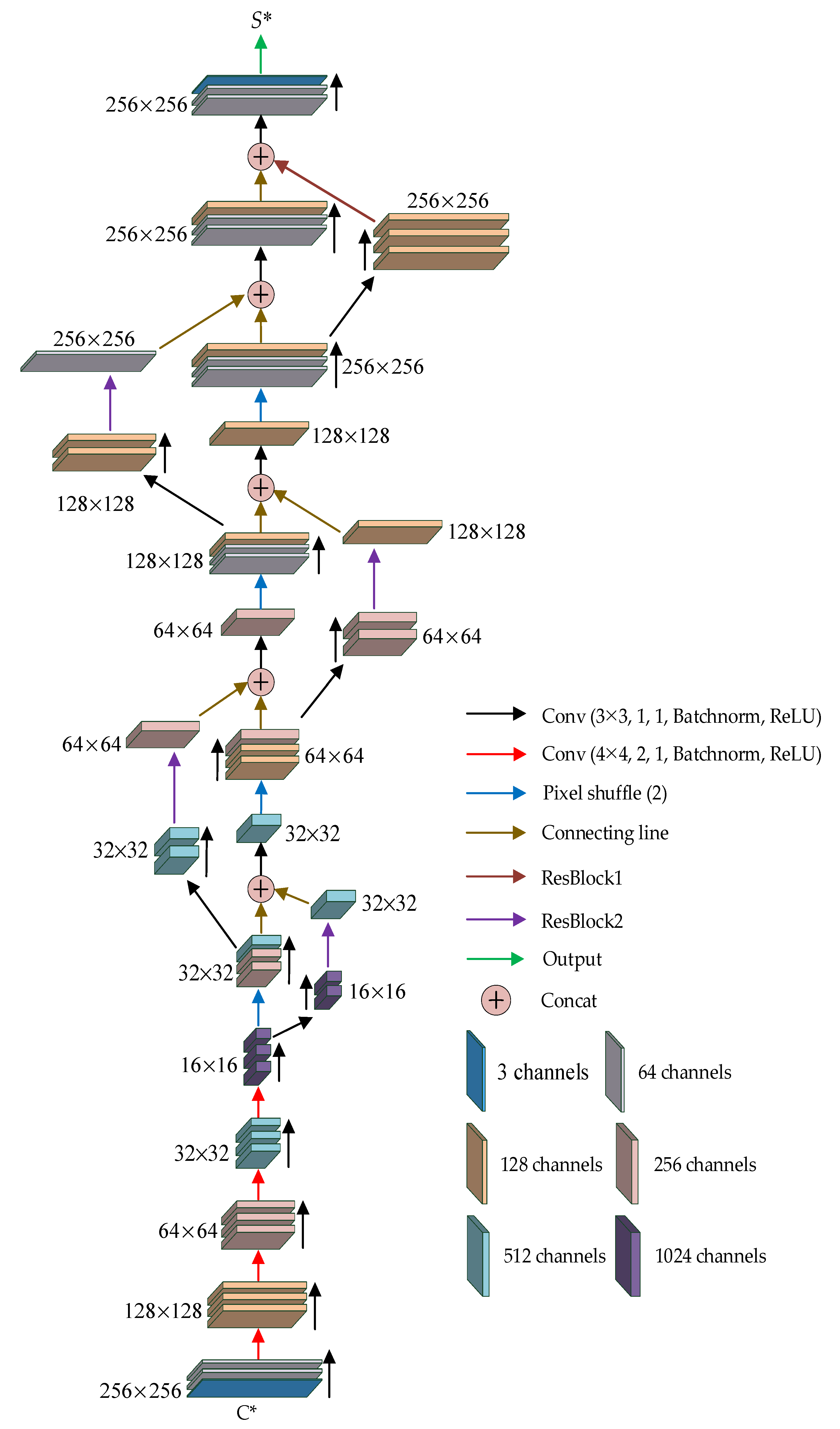
3.2. Recovery Network

The recovery network is also called Torch-Net because it is structured like a torch, as shown in Figure 4. It can be seen from Figure 4 that the container image was input from the low end, moved up along the lower pyramid, up the inverted pyramid, and, finally, reached the top, from which the reconstructed secret image was output. After every two convolutional layers, the size of the feature map was reduced to 1/4 of the original size using a third convolutional layer with a stride of 2. This operation was repeated four times, whereby the feature map was compressed from 256 × 256 to 16 × 16 and the number of channels was increased from 64 to 1024. Subsequently, the secret images were progressively reconstructed with the help of pixel shufflers and residual modules. On the one hand, the small-size feature map passed through a pixel shuffle layer and two convolution layers. On the other hand, it passed through two convolutional layers and an extended ResBlock2. Both operations enlarged the feature map by a factor of four. The two output feature maps were then concatenated. After five repetitions, the feature map size was restored to 256 × 256. In the fifth repetition, instead of using pixel shuffle and ResBlock2, an ordinary convolutional layer and ResBlock1 were used. Finally, after concatenating the two outputs, the reconstructed secret image was obtained.

4. Experimental Results

4.1. Developmental Environment and Dataset

The proposed Res-Hi-Netk was implemented using PyTorch (V. 1.10. Adam P.; Sam G.; Soumith C. Silicon Valley, USA) and accelerated using two GeForce RTX 3090Ti GPUs. The BOSSbase1.01 dataset [43] was used for training and testing (see Supplementary Materials). We resized the 50,000 original images in the dataset to a size of 256 × 256 and randomly divided the training set and test sets in a ratio of 4 to 1.

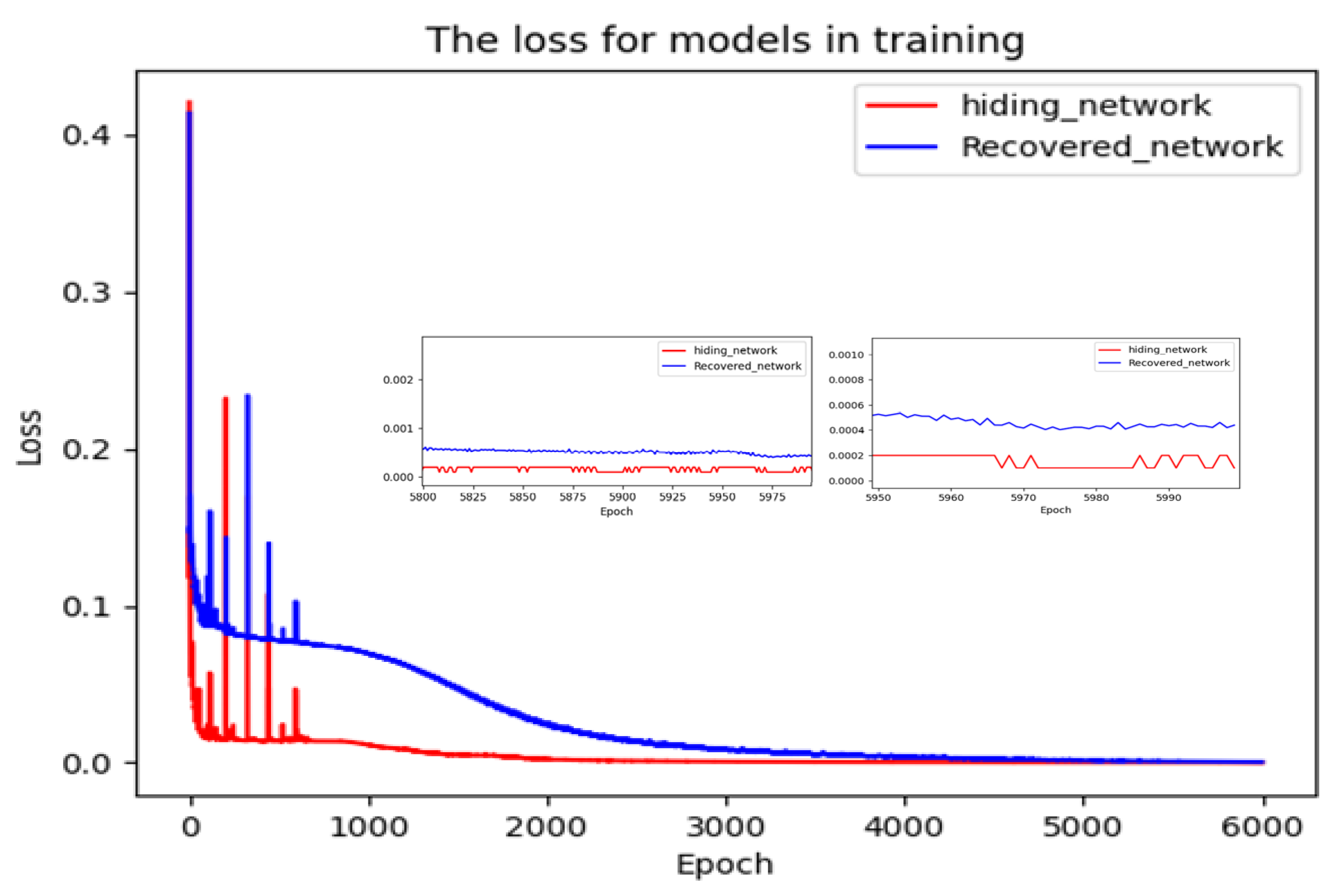
4.2. Training Process

During the training process, the hiding and recovery networks were trained together and constrained by the loss function. The loss function consisted of a loss function for the hiding network L₀ and a loss function for the recovery network L₁. When the final loss function met the requirements, the two models were saved and later used in a test set to verify the performance of the system. L₀ is defined as the l₁ norm of the difference between C and $\widehat{C}$.

$$L_0{=L}_0(C,\hat{C} )=\Vert C-\hat{C}\Vert ,$$

(1)

Besides, L₁ is used to control the difference between S and S*, and is defined as

$$L_1{=L}_1(S,S*)=\left|\right|S-S*\left|\right|.$$

(2)

Then the total loss function L is the weighted sum of L₀ and L₁,

$${L=L}_0{+\alpha L}_1.$$

(3)

where $\alpha$ is a balance factor.

The batch size was 8, the initial learning rate was set to 0.005 and $\alpha$ was 0.2 (It was determined by the ablation experiment in Section 4.6). Figure 5 shows the relationship between the training epoch and the loss function. It can be seen from the figure that more than 6000 epochs were trained, at which point the loss function converged. The whole training lasted for about 60 days. Figure 5 shows that the loss function L₀ decreased rapidly in the first 200 epochs and fluctuated in the next 600 epochs. Afterwards, it entered a slow downward trend and converged to 0.001 after 3000 epochs, and, finally, fell within the interval of 0.0001–0.0002. L₁ was similar to L₀, but the decline rate was slower than L₀, converging to about 0.0005 after 5800 epochs.

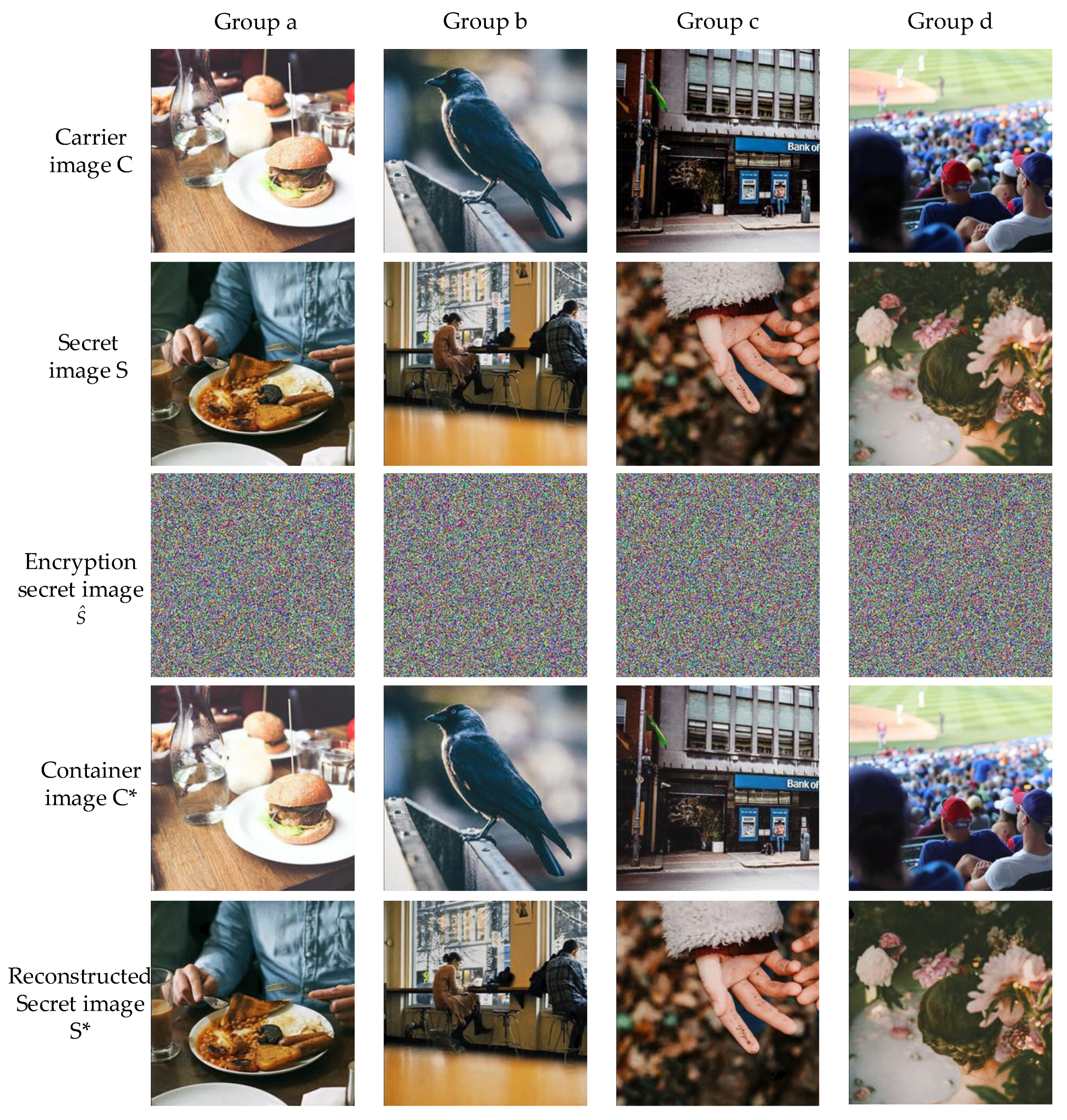
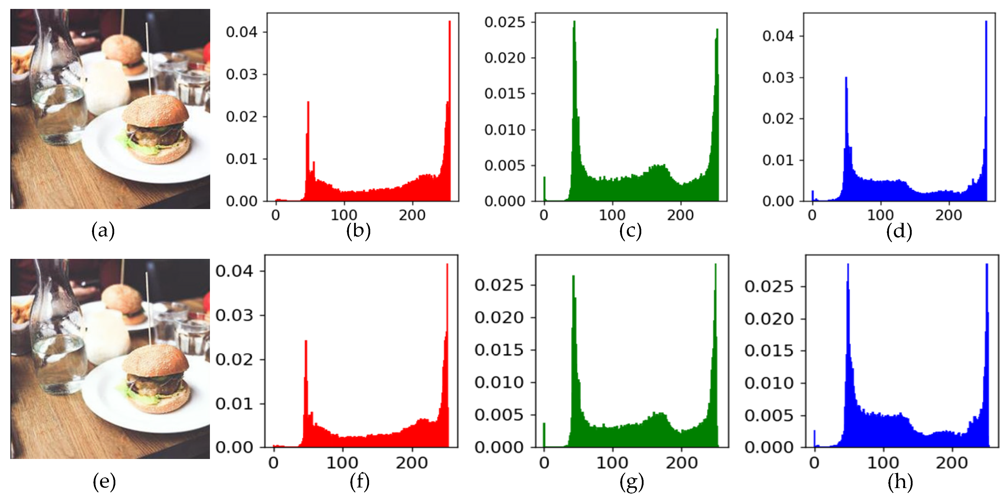
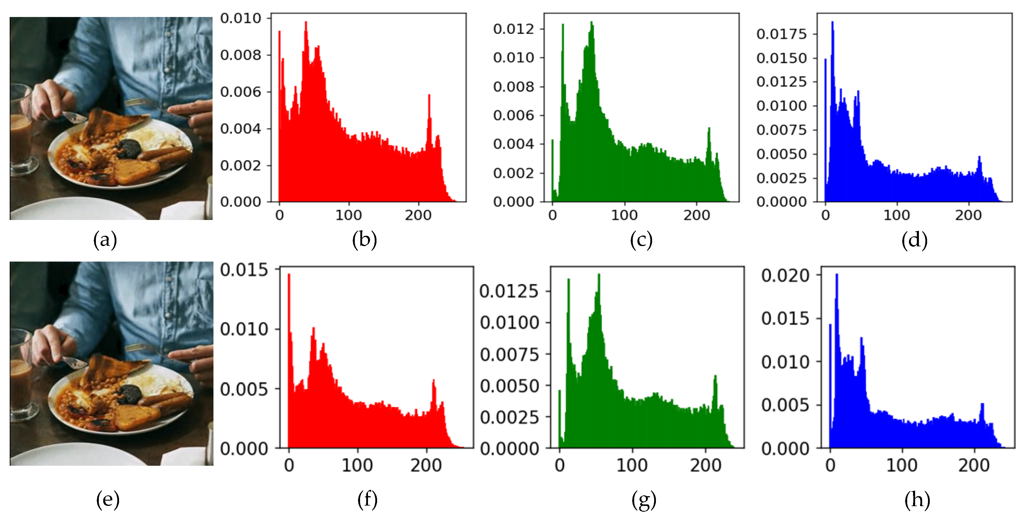
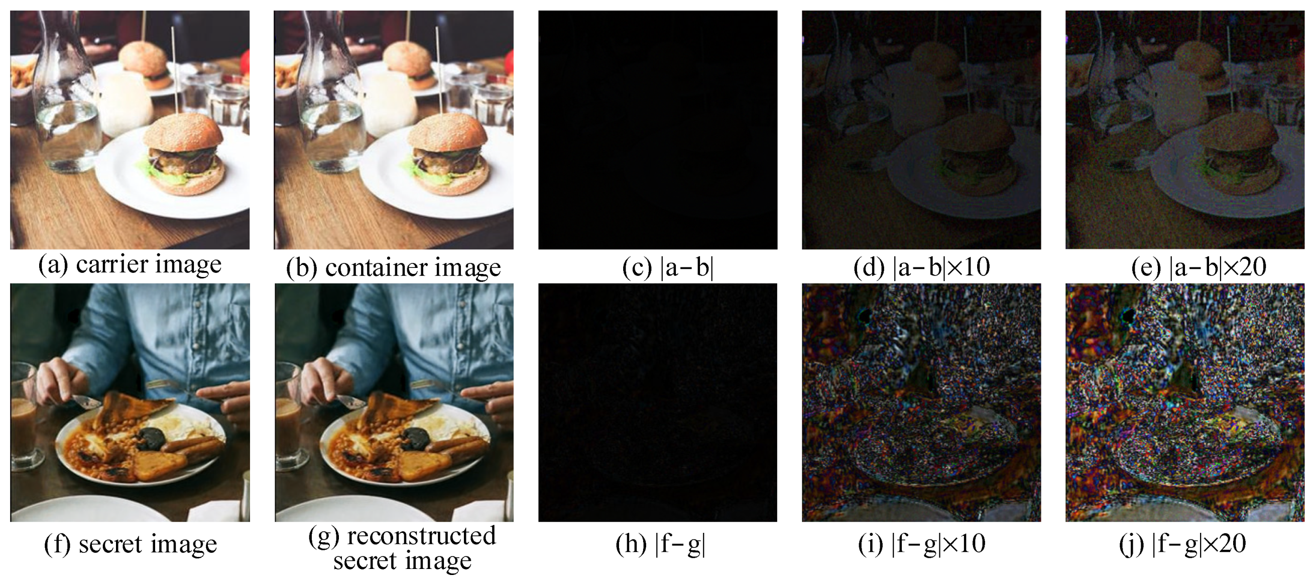
4.3. Results of Image Hiding and Recovery

Some of the results of image hiding and recovery are shown in Figure 6. Figure 6 shows four groups of images, each consisting of a carrier, a secret image, an encrypted secret image, a container, and the corresponding reconstructed secret image. Any container image in the fourth row cannot be distinguished from its corresponding carrier in the first row. As shown in Figure 7, the histograms of the three channels of the carrier images were almost identical to their corresponding container images. Similarly, Figure 8 shows the histograms of an original secret image and its reconstructed counterparts for the three channels. The histograms reflected the distribution of pixel values. This meant that the obtained container and reconstructed secret images had similar pixel distributions to their corresponding carrier and secret images.

Different images were used to measure the difference between two images. The first row of Figure 9 shows a carrier, a container and different images scaled by three factors of 1, 10 and 20. As can be seen in Figure 9, no information about the hidden image can be perceived, even when zoomed in. This showed the excellent hiding performance of the proposed algorithm. The difference images between the secret image and its corresponding reconstructed image are shown in the second row of Figure 9. This indicated that the proposed recovery network could successfully recover the hidden image.

The evaluation indexes, PSNR, MSE and MSSIM, as well as APE, for the four groups of test images in Figure 9, are listed in

Table 1. PSNR (dB) and images of MSSIM, MSE and APE (R, B, G).

Image Group	Container vs. Carrier PSNR (dB), MSSIM, MSE	Reconstructed vs. Secret PSNR (dB), MSSIM, MSE	Container vs. Carrier APE (R, G, B)	Reconstructed vs. Secret APE (R, G, B)
a	39.67, 0.99, 14.76	35.34, 0.96, 35.98	0.75, 0.78, 0.76	3.34,3.70, 3.73
b	40.51, 0.99, 10.78	32.30, 0.92, 114.91	0.45, 0.46, 0.55	5.29, 5.47, 6.32
c	40.22, 0.99, 11.34	35.29, 0.97, 45.86	0.53, 0.52, 0.54	3.91, 4.12, 4.58
d	40.34, 0.99, 12.31	34.61, 0.96, 53.57	0.64, 0.67, 0.66	4.00, 4.19, 4.61
Average	40.19, 0.99, 12.29	34.39, 0.95, 62.58	0.59, 0.61, 0.63	4.14, 4.37, 4.81

. It can be seen from Table 1 that between the carrier image and the container image, the average PSNR was greater than 40.19 dB, the MSSIM reached 0.99 on average, and the APE was less than 1 on average for all three channels. Between the reconstructed image and the original secret image, the average PSNR was 34.39 dB, the MSSIM reached 0.95 on average, and the average APEs for the R, G and B channels were 4.14, 4.37 and 4.81, respectively. This indicated that the performance of the proposed steganography network was excellent.

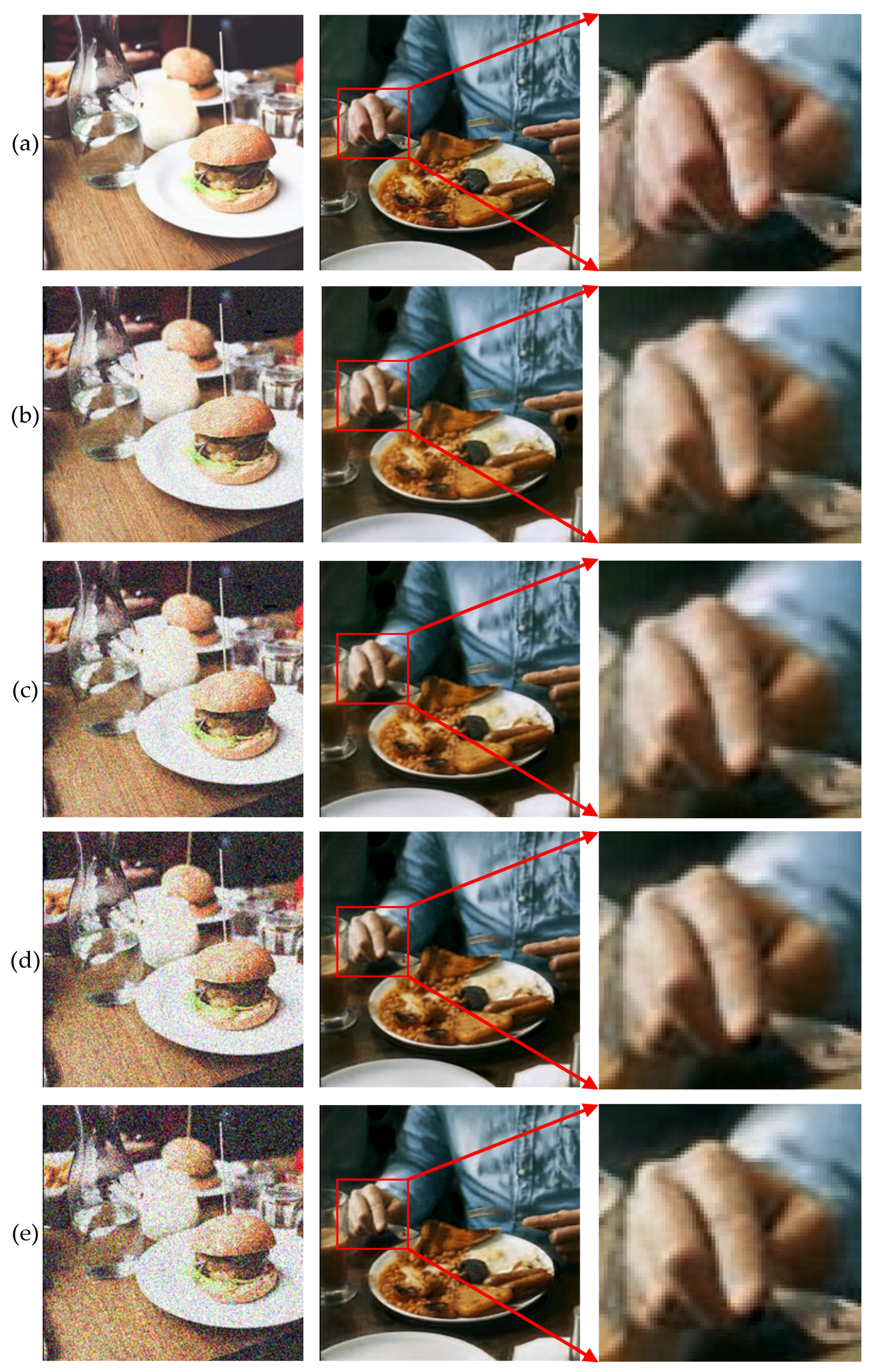
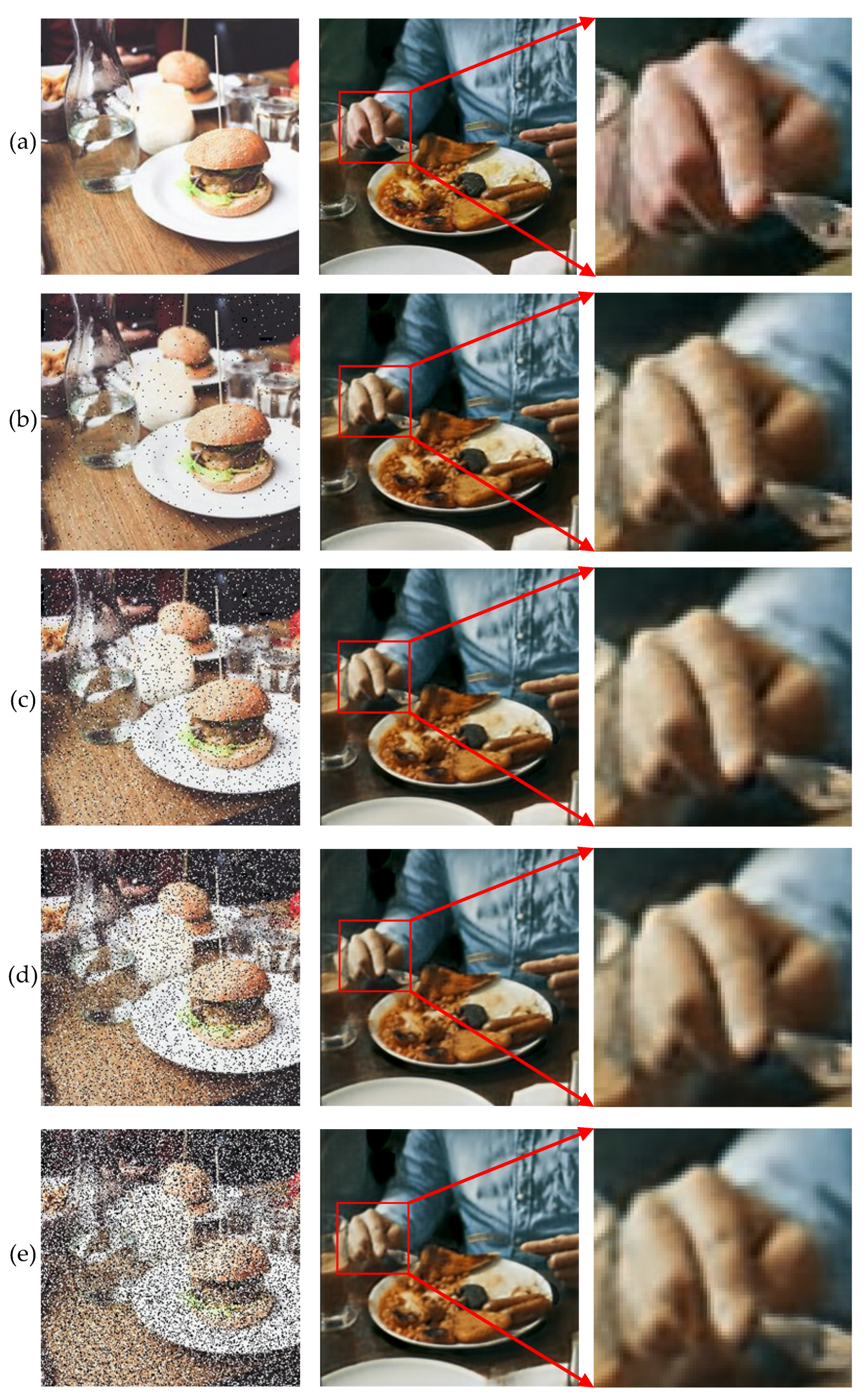
4.4. Performance of Resistance to Cropping and Noise Attacks

In this section, the performance of the recovery network in response to cropping attacks, as well as Gaussian and salt-and-pepper noise attacks, is discussed. Figure 10 shows the results of adding Gaussian noise with different intensities to the container images. As can be seen in Figure 10, the recovery network was able to reconstruct the secret images even with the addition of noise to the container images. As the intensity of the added noise increased, the quality of the reconstructed image became worse, but still acceptable with most of the details being perceptible. Even at a magnification of 16×, the edges of the reconstructed image became only slightly blurred. This could also be confirmed, as shown in

Table 2. Evaluation indexes of reconstructed secret images under container images with different noise attacks in Figure 10 and Figure 11.

Attack Mode	Attack Intensity	PSNR	MSSIM	MSE	APE (R, G, B)
Gaussian noise attack (power/dBW)	0.01	27.17	0.893	373	8.23, 7.88, 8.30
	0.04	26.75	0.875	415	8.87, 9.09, 9.52
	0.08	26.56	0.869	412	9.70, 8.60, 8.89
	0.12	26.31	0.857	455	9.85, 9.53, 9.84
Salt and pepper noise attack (power/dBW)	0.01	28.41	0.900	281	7.32, 7.22, 7.50
	0.05	27.86	0.893	320	7.77, 8.05, 8.41
	0.1	27.43	0.887	418	8.10, 8.27, 8.55
	0.2	25.03	0.863	612	9.51, 8.53, 9.06

, in which, of course, the quality metrics of the reconstructed secret image were worse than those of the secret image. However, when the added noise intensity was not significant, the PSNR and MSSIM were good enough, amounting to 27.17 dB and 0.893 for MSSIM, respectively. Another advantage was that the quality of the reconstructed secret image slowly decreased from 27.17 to 26.31 dB when the Gaussian noise intensity increased from 0.01 to 0.12 (12 times). As a result, the recovery network could somewhat resist the attack of Gaussian noise and recover high-quality secret images.

Figure 11 shows the results for different intensities of salt-and-pepper noise added to the container images. Similar to Gaussian noise, visually, when the intensity of the salt and pepper noise increased, the reconstructed network could still reconstruct the secret image, and most of the details were perceptible. When magnified 16 times, the loss of color and details could be found to be greater than in the case of Gaussian noise. From Table 2, it can be seen that the PSNR, MSSIM and APE indeed became worse with increasing intensity of the salt and pepper noise. However, the secret image was still acceptable, in terms of visual quality. When the noise intensity increased, the image quality decreased, but at a slower rate. Therefore, it could be concluded that the recovery network could resist the attack of salt and pepper noise to a certain extent and recover high-quality secret images.

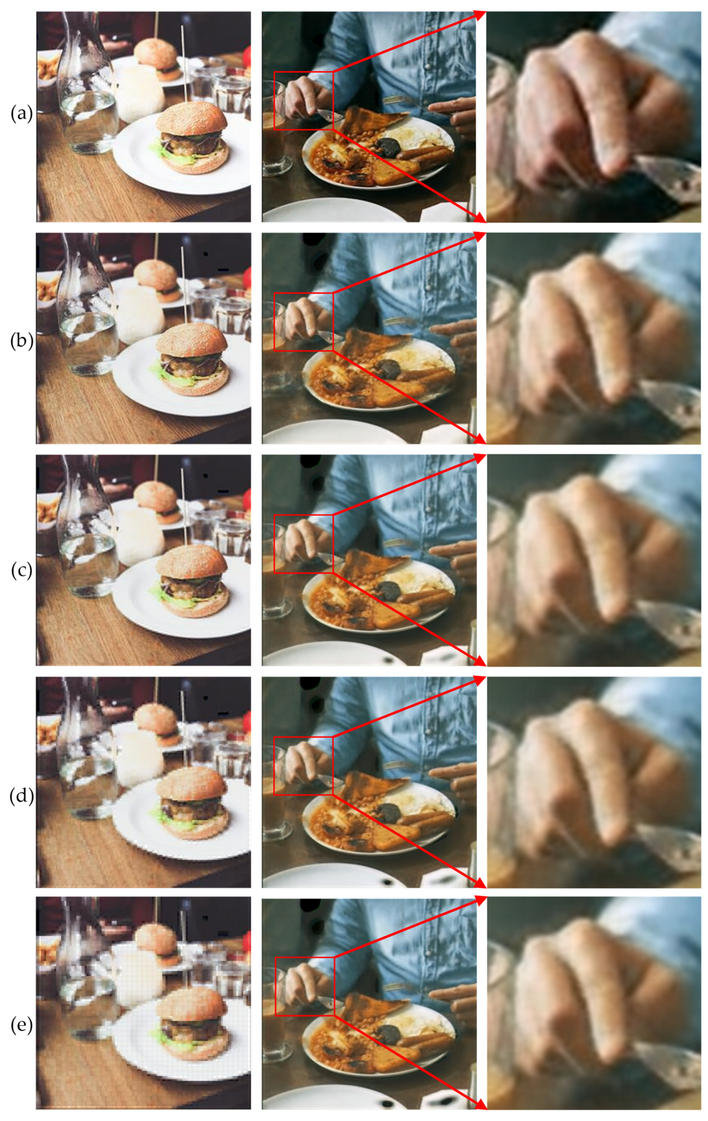
4.5. Performance of Resistance to Cropping and Compression Attacks

In this section, the performance of the recovery network in response to different cropping and compression attacks is discussed. Figure 12 shows the results with respect to the sizes of the cropped blocks in the container. The position of cropping was determined randomly. When the cutting size was small, such as 10 × 10 or 25 × 30, it was impossible to distinguish between the secret image reconstructed from the cropped container and the secret image reconstructed from the compressed container, and there was no visual difference between them. When the size of the cropping became larger, the reconstructed secret image became blurred as a whole, rather than the local blurring that occurred immediately around the corresponding cropping position, which indicated that the overall embeddedness of the secret image contributed to the reconstruction of the secret image, even in the case of partial loss of the container. The more the loss, the worse the quality of the recovery. This can also be seen from the image quality evaluation indicators in

Table 3. Evaluation indexes of the reconstructed secret images from container images in Figure 12 and Figure 13 subject to different attacks.

Attack Mode	Attack Intensity	PSNR (dB)	MSSIM	MSE	APE(R,G,B)
Cropping attacks (pixels)	10 × 10	31.98	0.963	126	3.43,3.33,3.53
	25 × 30	28.73	0.913	217	5.23,5.67,5.15
	Two of 25 × 30	25.56	0.844	588	9.98,9.08,10.56
	Three of 25 × 30	25.12	0.832	751	11.89,11,34,12.20
PCA compression (compression ratio)	1.53	24.32	0.835	1237	16.72,17.66,17.60
	2.98	23.14	0.822	1594	18.81,18.73,19,21
	5.88	21.51	0.806	1874	21.14,22.84,22.83
	11.77	20.63	0.783	2325	22.36,24.21,24.27

.

Figure 13 shows the results of the reconstructed secret image when the container was compressed at different compression ratios and then decompressed. It can be seen from Figure 13 that the compression of the container image had some impact on the quality of the reconstructed secret image. In the reconstructed secret image, some blocks became black. The larger the compression ratio was, the greater the number of black blocks there were. In addition, it can be seen from the data in Table 3 that the quality of the reconstructed secret images changed. When the compression ratio increased from 1.53 to 11.77, the PSNR decreased from 24.32 dB to 20.63 dB and the MSSIM decreased from 0.835 to 0.783. Meanwhile, the MSE rose rapidly and the APE of pixels became larger, but a slightly blurred reconstructed secret image could also be obtained. Visually, there were only subtle differences in color and edges between the reconstructed secret image and the secret image. Therefore, the proposed Resen-Hi-Net had certain resistance to cropping and compression attacks.

4.6. Resistance to Steganalyses

The ability to effectively resist steganalysis is a very important indicator of steganalysis algorithms. SRM [44], maxSRM [45] and Ye-Net [46] are three commonly used open source steganalysis algorithms. SRM and maxSRM are spatial domain-based image steganalysis tools. Ye-Net is a steganalysis model based on CNN. These three steganalysis algorithms were used to detect whether the extracted algorithm could effectively resist steganalysis. A total of 500 container images were randomly generated and tested using their corresponding carriers. The results are shown in Figure 14.

It is worth noting that when the secret images were encrypted and hidden in the carrier images, the secret images hidden in the container images were more difficult for the above steganalysis algorithms to detect. The results showed that our proposed Resen-Hi-Net with embedded pre-encryption was more robust to image steganalysis algorithms and improved the security of image steganography.

4.7. Ablation Study

To find a balance between hiding and recovery effects, we conducted ablation experiments on the parameters, $\alpha$, in the loss function. The results of steganography and steganalysis were calculated for 1000 groups of images, as shown in

Table 4. Average PSNR and MSSIM between carriers and containers, as well as reconstructed secret images and secret images for different α values, and average AUC for attacking containers using different steganalysis algorithms.

$\mathit{\alpha }$	Container vs. Carrier		Reconstructed vs. Secret		AUC
	PSNR (dB)	MSSIM	PSNR (dB)	MSSIM	SRM	MaxSRM	Ye-Net
1	37.98	0.973	37.68	0.971	0.67	0.76	0.81
0.8	38.73	0.978	36.42	0.968	0.66	0.73	0.79
0.6	39.16	0.984	36.13	0.964	0.63	0.69	0.76
0.4	39.75	0.988	35.53	0.963	0.57	0.63	0.73
0.2	40.60	0.993	34.23	0.960	0.51	0.58	0.69
0.1	41.39	0.994	32.07	0.952	0.51	0.57	0.64

. Table 4 shows that when $\alpha$ = 0.2, the probability of 69% could be detected by steganalysis, and with the increase of a, the probability of detection also increased. When $\alpha$ = 0.1, although the probability of detection was reduced, the quality of the reconstructed secret image was poor and many details were lost. Considering comprehensively, $\alpha$ was taken as 0.2.

4.8. Comparison with Other State-of-the-Art CNN Steganography Approaches

In this section, the proposed algorithm was compared with other state-of-the-art CNN approaches, as shown in

Table 5. Comparative experimental results of the proposed, Baluja-Net [34] and ISN [35] hiding algorithms.

Methods	Container vs. Carrier			Reconstructed vs. Secret			Against Steganalysis (AUC)
	PSNR (dB)	MSSIM	APE (R,G,B)	PSNR (dB)	MSSIM	APE (R,G,B)	SRM	MaxSRM	Ye-Net
Baluja-Net [34]	36.49	0.95	0.48, 0.49, 0.43	30.56	0.90	4.79, 4,37, 4.53	0.63	0.72	0.79
ISN [35]	39.28	0.977	N/A	40.42	0.985	N/A	0.59	0.65	0.73
Proposed Resen-Hi-Net	40.13	0.983	0.45, 0.46, 0.44	34.25	0.951	3.95, 4.34, 4.46	0.51	0.58	0.69

. The results in Table 5 were the average experimental results for 100 groups of container and carrier images.

As can be seen from Table 5, the steganography performance of our model outperformed the other two methods in terms of resistance to steganalysis algorithms. Specifically, the AUCs of the proposed model were 0.51, 0.58 and 0.69 in resisting the steganalysis algorithms of SRM, MaxSRM and Ye-Net, respectively, which were lower than the other two image hiding methods of Baluja-Net and ISN. This implied that the proposed Resen-Hi-Net had the least possibility of being broken. In addition, the performance of recovery of the proposed model was the same as that of Baluja-Net, but slightly worse than that of ISN.

5. Conclusions and Discussion

A new highly secure image hiding algorithm, Resen-Hi-Net, is proposed. The secret image is encrypted and then hidden in the carrier image to obtain the container image. The encrypted secret image has a uniform distribution of pixel values and is visually a white noise-like image. The resulting container image cannot be visually distinguished from the carrier image. Furthermore, the recovery network can effectively reconstruct high-quality secret images. In the comparative experiments, the proposed algorithm could better resist steganalysis algorithm detection, as well as noise, clipping, compression and other attacks. The proposed Resen-Hi-Net performed well in terms of steganography metrics, such as PSNR, MSSIM and other indicators, between container and carrier images and between reconstructed and original secret images. In addition, it had a certain degree of resistance to several commonly used steganalysis algorithms and common attacks, such as cropping, noise and compression attacks. Consequently, the proposed Resen-Hi-Net is stable in terms of resistance to different attacks and reversible in terms of its ability to recover secret images.

References

1. Piao, Y.R.; Shin, D.H.; Kim, E.S. Robust image encryption by combined use of integral imaging and pixel scrambling techniques. Opt. Lasers Eng. 2009, 47, 1273–1281. [Google Scholar] [CrossRef]
2. Ye, G.D. Image scrambling encryption algorithm of pixel bit based on chaos map. Pattern Recognit. Lett. 2010, 31, 347–354. [Google Scholar] [CrossRef]
3. Zhou, Y.; Li, C.L.; Li, W.; Li, H.; Feng, W.; Qian, K. Image encryption algorithm with circle index table scrambling and partition diffusion. Nonlinear Dyn. 2021, 103, 2043–2061. [Google Scholar] [CrossRef]
4. Cariolaro, G.; Erseghe, T.; Kraniauskas, P. The fractional discrete cosine transform. IEEE Trans. Signal Process. 2002, 50, 902–911. [Google Scholar] [CrossRef]
5. Wu, J.H.; Zhang, L.; Zhou, N.R. Image encryption based on the multiple-order discrete fractional cosine transform. Opt. Commun. 2010, 283, 1720–1725. [Google Scholar] [CrossRef]
6. Wu, J.H.; Guo, F.F.; Zeng, P.P. Image encryption based on a reality-preserving fractional discrete cosine transform and a chaos-based generating sequence. J. Mod. Opt. 2013, 60, 1760–1771. [Google Scholar] [CrossRef]
7. Xu, Y.; Wang, H.; Li, Y.G.; Pei, B. Image encryption based on synchronization of fractional chaotic systems. Commun. Nonlinear Sci. 2014, 19, 3735–3744. [Google Scholar] [CrossRef]
8. Chen, L.F.; Zhao, D.M. Optical image encryption based on fractional wavelet transform. Opt. Commun. 2005, 254, 361–367. [Google Scholar] [CrossRef]
9. Tao, R.; Meng, X.Y.; Wang, Y. Image encryption with multi orders of fractional Fourier transforms. IEEE Trans. Inf. Forensics Secur. 2010, 5, 734–738. [Google Scholar] [CrossRef]
10. Hennelly, B.M.; Sheridan, J.T. Image encryption and the fractional Fourier transform. Optik 2003, 114, 251–265. [Google Scholar] [CrossRef]
11. Zhou, N.R.; Dong, T.J.; Wu, J.H. Novel image encryption algorithm based on multiple-parameter discrete fractional random transform. Opt. Commun. 2010, 283, 3037–3042. [Google Scholar] [CrossRef]
12. Hussain, M.; Wahab, A.W.A.; Idris, Y.I.B.; Ho, A.T.; Jung, K.H. Image steganography in spatial domain: A survey. Signal Process. Image 2018, 65, 46–66. [Google Scholar] [CrossRef]
13. Djebbar, F.; Ayad, B.; Hamam, H.; Abed-Meraim, K. A view on latest audio steganography techniques. In Proceedings of the International Conference on Innovations in Information Technology, Abu Dhabi, United Arab Emirates, 25–27 April 2011. [Google Scholar] [CrossRef]
14. Fang, T.; Jaggi, M.; Argyraki, K. Generating steganographic text with LSTMs. arXiv 2017, arXiv:1705.10742v1. [Google Scholar]
15. Balaji, R.; Naveen, G. Secure data transmission using video steganography. In Proceedings of the Asia International Conference on Modelling & Simulation, Mankato, MN, USA, 15–17 May 2011. [Google Scholar] [CrossRef]
16. Wang, Z.H.; Yang, H.R.; Cheng, T.F.; Chang, C.C. A high-performance reversible data-hiding scheme for LZW codes. Appl. Res. Comput. 2013, 86, 2771–2778. [Google Scholar] [CrossRef]
17. Bender, W.R.; Gruhl, D.; Morimoto, N. Techniques for data hiding, storage and retrieval for image and video databases III. Int. Soc. Opt. Photonics 1996, 35, 313–336. [Google Scholar] [CrossRef]
18. Westfeld, A.; Pfitzmann, A. Attacks on steganographic systems-breaking the steganographic utilities EzStego, Jsteg, Steganos, and s-tools-and some lessons learned. In Proceedings of the International Workshop on Information Hiding, Dresden, Germany, 29 September–1 October 1999. [Google Scholar] [CrossRef]
19. Westfeld, A. F5–a steganographic algorithm. In Proceedings of the International Workshop on Information Hiding, Pittsburgh, PA, USA, 25–27 April 2001. [Google Scholar] [CrossRef]
20. Filler, T.; Judas, J.; Fridrich, J. Minimizing additive distortion in steganography using syndrome-trellis codes. IEEE Trans. Inf. Forensics Secur. 2011, 6, 920–935. [Google Scholar] [CrossRef]
21. Pevný, T.; Filler, T.; Bas, P. Using high-dimensional image models to perform highly undetectable steganography. In Proceedings of the International Conference, Calgary, AB, Canada, 28 June 2010; Available online: http://boss.gipsa-lab.grenoble-inp.fr/BOSSRank/ (accessed on 1 July 2010).
22. Holub, V.; Fridrich, J. Designing steganographic distortion using directional filters. In Proceedings of the Information Forensics and Security, Costa Adeje, Spain, 2–5 December 2012. [Google Scholar] [CrossRef]
23. Holub, V.; Fridrich, J. Digital image steganography using universal distortion. In Proceedings of the First ACM Workshop on Information Hiding and Multimedia Security, Montpellier, France, 17–19 June 2013. [Google Scholar] [CrossRef]
24. Volkhonskiy, D.; Borisenko, B.; Burnaev, E. Generative adversarial networks for image steganography. In Proceedings of the International Conference on Learning Representations, San Juan, Puerto Rico, 2–4 May 2016; Available online: https://openreview.net/pdf?id=H1hoFU9xe (accessed on 1 June 2016).
25. Goodfellow, I.J.; Pouget-Abadie, J.; Mirza, M.; Xu, B.; Warde-Farley, D.; Ozair, S.; Courville, A.; Bengio, Y. Generative adversarial networks. Adv. Neural Inf. Processing Syst. 2014, 3, 2672–2680. Available online: https://arxiv.org/pdf/1406.2661.pdf (accessed on 10 June 2014). [CrossRef]
26. Shi, H.; Dong, J.; Wang, W.; Qian, Y.; Zhang, X. SSGAN: Secure steganography based on generative adversarial networks. In Advances in Multimedia Information Processing; Springer: Cham, Switzerland, 10 May 2017. [Google Scholar] [CrossRef]
27. Yang, J.; Kai, L.; Kang, X.; Wong, E.K.; Shi, Y.Q. Spatial image steganography based on generative adversarial network. arXiv 2018, arXiv:1804.07939. [Google Scholar]
28. Wang, Z.; Gao, N.; Wang, X.; Xiang, J.; Zha, D.; Li, L. Hiding GAN: High-capacity information hiding with generative adversarial network. Comput. Graph. Forum. 2019, 38, 393–401. [Google Scholar] [CrossRef]
29. Li, C.; Jiang, Y.; Cheslyar, M. Embedding image through generated intermediate medium using deep convolutional generative adversarial network. Comput. Mater. Continua. 2018, 56, 313–324. [Google Scholar] [CrossRef]
30. Qin, J.; Wang, J.; Tan, Y. He, Z. Coverless image steganography based on generative adversarial network. Mathematics 2020, 8, 1394. [Google Scholar] [CrossRef]
31. Baluja, S. Hiding images in plain sight: Deep steganography. In Proceedings of the Advances in Neural Information Proceeding Systems, Long Beach, CA, USA, 4–9 December 2017. [Google Scholar] [CrossRef]
32. Rehman, A.U.; MSNadeem, R.R.; Su, H. End-to-end trained CNN encode-decoder networks for image steganography. arXiv 2017, arXiv:1711.07201v1. [Google Scholar]
33. Wang, Z.; Gao, N.; Wang, X.; Xiang, J.; Liu, G. Stnet: A style transformation network for deep image steganography. In Proceedings of the International Conference on Neural Information Processing, Sydney, NSW, Australia, 12–15 December 2019. [Google Scholar] [CrossRef]
34. Baluja, S. Hiding images within images. IEEE Trans. Pattern Anal. Mach. Intell. 2020, 42, 1685–1697. [Google Scholar] [CrossRef] [PubMed]
35. Lu, S.P.; Wang, R.; Zhong, T.; Rosin, P.L. Large-capacity image steganography based on invertible neural networks. In Proceedings of the 34th IEEE Conference on Computer Vision and Pattern Recognition, Kuala Lumpur, Malaysia, 19–25 June 2021. [Google Scholar] [CrossRef]
36. Zhu, X.; Lai, Z.; Liang, Y.; Xiong, J.; Wu, J. Generative high-capacity image hiding based on residual CNN in wavelet domain. Appl. Soft Comput. 2022, 115, 108170. [Google Scholar] [CrossRef]
37. He, K.M.; Zhang, X.Y.; Ren, S.Q.; Sun, J. Deep residual learning for image recognition. In Proceedings of the IEEE Conference on Computer Vision and Pattern Recognition, Las Vegas, NV, USA, 27–30 June 2016. [Google Scholar] [CrossRef]
38. Wang, G.; Zeng, G.D.; Cui, X.Y.; Feng, S. Dispersion analysis of the gradient weighted finite element method for acoustic problems in one, two, and three dimensions. Int. J. Numer. Meth. Eng. 2019, 120, 473–497. [Google Scholar] [CrossRef]
39. Yue, L.; Shen, H.; Li, J.; Yuan, Q.; Zhang, H.; Zhang, L. Image super-resolution: The techniques, applications, and future. Signal Proces. 2016, 128, 389–408. [Google Scholar] [CrossRef]
40. Wu, J.; Xia, W.; Zhu, G.; Liu, H.; Ma, L.; Xiong, J. Image encryption based on adversarial neural cryptography and SHA controlled chaos. J. Mod. Opt. 2021, 68, 409–418. [Google Scholar] [CrossRef]
41. Welstead, S.T. Fractal and wavelet image compression techniques. SPIE Opt. Eng. Press. 1999, 155–156. [Google Scholar] [CrossRef]
42. Wang, Z.; Bovik, A.C.; Sheikh, R.; Simoncelli, E.P. Image quality assessment: From error visibility to structural similarity. IEEE Trans. Image Process. 2004, 13, 600–612. [Google Scholar] [CrossRef]
43. Bas, P.; Filler, T.; Pevny, T. Break our steganographic system: The ins and outs of organizing BOSS. In Proceedings of the 13th International Conference on Information Hiding, Prague, Czech Republic, 18–20 May 2011. [Google Scholar] [CrossRef]
44. Fridrich, J.; Kodovský, J. Rich models for steganalysis of digital images. IEEE Trans. Inf. Forensics Secur. 2012, 7, 868–882. [Google Scholar] [CrossRef]
45. Denemark, T.; Sedighi, V.; Holub, V.; Holub, V.; Cogranne, R.; Fridrich, J. Selection-channel-aware rich model for steganalysis of digital image. IEEE Trans. Inf. Forensics Secur. 2014, 48–53. [Google Scholar] [CrossRef]
46. Ye, J.; Ni, J.Q.; Yi, Y. Deep learning hierarchical representations for image steganalysis. IEEE Trans. Inf. Foren. Sec. 2017, 12, 2545–2557. [Google Scholar] [CrossRef]
Figure 1. Two ResBlocks (Conv: Convolutional network, Concat: Concatenation operation, Deconv: Deconvolutional network).
Mathematics 10 02934 g001
Figure 2. Steganography algorithm flowchart.
Mathematics 10 02934 g002
Figure 3. Hiding network structure (Conv: Convolutional network, Concat: Concatenation operation).
Mathematics 10 02934 g003
Figure 4. Torch-Net structure (Conv: Convolutional network, Concat: Concatenation operation).
Mathematics 10 02934 g004
Figure 5. Loss function curves of hiding and recovery networks.
Mathematics 10 02934 g005
Figure 6. Results of the four tests for image hiding and reconstruction.
Mathematics 10 02934 g006
Figure 7. Histogram comparison between a carrier image and a container image: (a) carrier image; (bd) histograms of pixel values of (a) for the three (RGB) channels, respectively; (e) container image; (fh) histograms of pixel values of (e) for the three (RGB) channels, respectively.
Mathematics 10 02934 g007
Figure 8. Histogram comparison between a secret image and a reconstructed secret image: (a) secret image; (bd) histograms of pixel values of (a) for the three (RGB) channels, respectively; (e) reconstructed secret image; (fh) histograms of pixel values of (e) for the three (RGB) channels, respectively.
Mathematics 10 02934 g008
Figure 9. Difference images between carrier and container images, and secret and reconstructed secret images.
Mathematics 10 02934 g009
Figure 10. Recovery results of secret images with different intensities of Gaussian noise added to container images: (a) 0, (b) 0.01, (c) 0.04, (d) 0.08 and (e) 0.12 dBW. From left to right correspond to containers, reconstructed secret images and magnified hand areas in the reconstructed images, respectively.
Mathematics 10 02934 g010
Figure 11. Recovery results of secret images with different intensities of salt-and-pepper noise added to container images: (a) 0, (b) 0.01, (c) 0.05, (d) 0.1 and (e) 0.2 dBW. From left to right correspond to containers, reconstructed secret images and magnified hand areas in the reconstructed images, respectively.
Mathematics 10 02934 g011
Figure 12. Comparison of reconstructed secret images from containers cropped at different sizes (the black areas indicate the cropped area): (a) no cropping, (b) 10 × 10, (c) 25 × 30, (d) two of 25 × 30, and (e) three of 25 × 30. From left to right correspond to cropped containers, reconstructed secret images, and magnified hand areas in the reconstructed secret images, respectively.
Mathematics 10 02934 g012
Figure 13. Comparison of secret images reconstructed from container images with different compression ratios: (a) 1, (b) 1.53, (c) 2.98, (d) 5.88 and (e) 11.77. From left to right correspond to compressed containers, reconstructed secret images, and magnified hand areas in the reconstructed secret images, respectively.
Mathematics 10 02934 g013
Figure 14. ROC and AUC detected by SRM, maxSRM and Ye-Net steganalysis algorithms.
Mathematics 10 02934 g014