The Shape Parameter in the Shifted Surface Spline—An Easily Accessible Approach

Abstract

In this paper, we present an easily accessible approach to finding a suitable shape parameter in the shifted surface spline for function interpolation. We aim at helping more readers, including mathematicians and non-mathematicians, to use our method to solve practical problems. Hence, some highly complicated mathematical theorems and definitions are avoided. The major requirement, as in our previous approach, that the data points should be evenly spaced in the domain is also relaxed. This means that the data points are purely scattered without restrictions. The drawback is that the shape parameter thus obtained is not exactly the same as the theoretically predicted optimal value, which can always be achieved by using our previous rigorous approach. However, experiments show that the gap is quite small and the final interpolation errors thus obtained are satisfactory.

1. Introduction

In the field of radial basis functions (RBF), one of the most frequently used basis functions is the shifted surface spline, defined by

$$\begin{array}{ccc}\hfill h\left(x\right)& :=& \left\{\begin{array}{cc}{(-1)}^{\lceil m\rceil }{\left(\right|x|}^2+c^2{)}^{\frac{\lambda }{2}},\lambda \in {\mathbb{Z}}_{+},\lambda \mathrm{odd},m=\frac{\lambda }{2}\hfill & \mathrm{if}n\mathrm{is}\mathrm{odd},\hfill \\ {(-1)}^m{\left(\right|x|}^2+c^2{)}^{\frac{\lambda }{2}}log{\left(\right|x|}^2+c^2{)}^{\frac{1}{2}},\lambda \in {\mathbb{Z}}_{+},\lambda \mathrm{even},m=1+\frac{\lambda }{2}\hfill & \mathrm{if}n\mathrm{is}\mathrm{even},\hfill \end{array}\right.\hfill \end{array}$$

(1)

where $x\in {\mathbb{R}}^n$, $c>0$, $\left|x\right|$ stands for the Euclidean norm of x, log denotes the natural logarithm, $\lceil m\rceil$ denotes the smallest integer not less than m, and $\lambda ,c$ are constants determined by the user. The latter are called shape parameters and greatly influence the quality of the approximation. From the viewpoint of computation, for even dimensions, $\lambda$ should be as small as possible. Hence, we will let it be two in this paper whenever possible, especially in the experiment. As for c, its choice is a challenge. If this problem remains unsolved, the power of this radial function will be greatly limited.

The function $h\left(x\right)$ defined in Equation (1) is obtained from the fundamental solution of the iterated Laplacian by the shifting $\left|x\right|\to {\left(\right|x|}^2+c^2{)}^{1/2},$ with $c>0$ (Dyn [1] and Yoon [2,3]). Its generalized Fourier transform is

$$\begin{array}{c}\hfill \widehat{h}\left(\xi \right)={l(\lambda ,n)\left|\xi \right|}^{-\lambda -n}{\tilde{\mathcal{K}}}_{\frac{n+\lambda }{2}}\left(c\right|\xi \left|\right),\end{array}$$

(2)

where $l(\lambda ,n)$ is a constant depending on $\lambda ,n$ (see Luh [4]), and ${\tilde{\mathcal{K}}}_{\nu }\left(t\right):=t^{\nu }{\mathcal{K}}_{\nu }\left(t\right),{\mathcal{K}}_{\nu }$ being the modified Bessel function of the second kind (Abramowitz et al. [5]). This Fourier transform will be needed in our main theorem. Moreover, it shows that, from the viewpoint of the Fourier transform, the well-known multiquadrics are simply a type of shifted surface spline, because they share the same Fourier transform as in Equation (2).

For odd dimensions, $h\left(x\right)$ is generally called the multiquadric. For multiquadrics, the choice of the shape parameter c has been dealt with by the author ([6]). In this paper, we will focus on even dimensions. Hereafter, whenever referring to Equation (1), we will mean $h\left(x\right)$ for even dimensions only.

One of the main advantages of the RBF approach for function interpolation is that it is mesh-free. For any set of scattered data points $(x_1,f\left(x_1\right)),\dots ,(x_N,f\left(x_N\right))$, where $x_1,\dots ,x_N$ are arbitrary points in ${\mathbb{R}}^n$ and $f\left(x_1\right),\dots ,f\left(x_N\right)$ are arbitrary real numbers, one can always find a unique interpolator of the form

$$s\left(x\right):=\sum _{j=1}^N{c}_{j}h(x-x_j)+p\left(x\right)$$

(3)

interpolating these data points, where $c_1,\dots ,c_N$ are constants to be determined and p is a polynomial of degree $\le m-1$. The only requirement for the data points is that $x_1,\dots ,x_N$ should be polynomially nondegenerate; that is, the only polynomial that vanishes at $x_1,\dots ,x_N$ is the zero polynomial. The detailed theory can be seen in Wendland [7] and Buhmann [8].

When using Equation (1), we already have a theoretically rigorous and practically useful method to choose the optimal shape parameter c contained in h, as introduced in Luh [4]. However, there is a severe restriction in [4] that the interpolation centers $x_1,\dots ,x_N$ should be evenly spaced in a simplex. This, to some extent, means that meshes are still needed. Moreover, the function domain must be a simplex. In this paper, we completely discard the two requirements and develop a new approach for finding a suitable c.

2. Materials and Methods

In order to make this paper self-contained, without overly referring to the complicated theory in [4], next, we recall its main results as in the following subsection.

2.1. The Orthodox Approach

Two definitions governing the distribution of the interpolation points are needed.

Definition 1.

Let E be an n-dimensional simplex in ${\mathbb{R}}^n$ with vertices $v_1,\dots ,v_{n+1}$ (see, e.g., [9]). For any point $x\in E$, its barycentric coordinates are the non-negative numbers ${\lambda }_1,\dots ,{\lambda }_{n+1}$ satisfying

$$x=\sum _{i=1}^{n+1}{\lambda }_i{v}_i,\sum _{i=1}^{n+1}{\lambda }_i=1.$$

Now, we need a parameter, called the degree, which indicates the amount of interpolation points in the domain. The larger the degree is, the more points are used.

Definition 2.

For any natural number k, the corresponding domain points of E of degree k are the evenly spaced points with barycentric coordinates

$$(k_1/k,k_2/k,\dots ,k_{n+1}/k)with{k}_1+\cdots +k_{n+1}=k.$$

As pointed out in Luh [4], the number of such points is equal to the dimension of ${\mathbb{P}}_k^n$, the space of n-variate polynomials of degree less than or equal to k. In this subsection, we use N to denote this number. Thus, $N:=dim{\mathbb{P}}_k^n$.

Two constants involved in the main theorem should be defined here.

Definition 3.

Let h be as in Equation (1). The constants ρ and ${\Delta }_0$ are defined as follows.

(a) 

Suppose $n-\lambda >3$. Let $q:=\lceil \frac{n-\lambda -3}{2}\rceil$, the smallest integer not less than $\frac{n-\lambda -3}{2}$. Then,

$$\rho :=1+\frac{q}{2m+3}and{\Delta }_0:=\frac{(2m+2+q)(2m+1+q)\cdots (2m+3)}{{\rho }^{2m+2}}.$$

(b) 

Suppose $n-\lambda \le 1$. Let $q:=-\lceil \frac{n-\lambda -3}{2}\rceil$. Then,

$$\rho :=1and{\Delta }_0:=\frac{1}{(2m+2)(2m+1)\cdots (2m-q+3)}.$$

(c) 

Suppose $1<n-\lambda \le 3$. Then, $\rho :=1and{\Delta }_0:=1.$

The approximated functions lie in the so-called native space ${\mathcal{C}}_{h,m}$. We refer to Luh, Madych and Nelson [10,11,12] and Wendland [7] for its definition. For such functions, we have the following main theorem describing the upper bound for the interpolation error.

Theorem 1.

Let h be as in Equation (1). For any positive number $b_0$, there exist positive constants ${\delta }_0,c_1,C,\omega ,0<\omega <1$, completely determined by h and $b_0$, such that, for any n-dimensional simplex $Q_0$ of diameter $b_0$, any $f\in {\mathcal{C}}_{h,m}$, and any $0<\delta \le {\delta }_0$, there exists a number r satisfying the property that $\frac{1}{3C}\le r\le b_0$, and, for any n-dimensional simplex Q of diameter r, $Q\subseteq Q_0$, there is an interpolating function $s(·)$ as defined in Equation (3) such that

$$|f\left(x\right)-s\left(x\right)|\le c_1\sqrt{\delta }{\left(\omega \right)}^{\frac{1}{\delta }}{\parallel f\parallel }_h$$

(4)

for all x in Q, where C is defined by

$$C:=max\left\{8{\rho }^{\prime },\frac{2}{3b_0}\right\},{\rho }^{\prime }:=\frac{\rho }{c},$$

where ρ and c appeared in Definition 3 and Equation (1), respectively. The function $s(·)$ interpolates f at $x_1,\dots ,x_N$, which are evenly spaced points of degree $k-1$ on Q as defined in Definition 2, with $k=\lceil \frac{r}{\delta }\rceil$. Here, ${\parallel f\parallel }_h$ is the h-norm of f in the native space.

The numbers ${\delta }_0,c_1$ and ω are given by ${\delta }_0:=\frac{1}{3C(m+1)}$, where m appeared in Equation (1),

$$c_1:=\sqrt{l(\lambda ,n)}{\left(2\pi \right)}^{\frac{1}{4}}\sqrt{n{\alpha }_n}{c}^{\frac{\lambda }{2}}\sqrt{{\Delta }_0}\sqrt{3C}\sqrt{{\left(16\pi \right)}^{-1}}$$

where λ is as in Equation (1), $l(\lambda ,n)$ appeared in Equation (2), ${\alpha }_n$ is the volume of the unit ball in ${\mathbb{R}}^n$, and ${\Delta }_0$ was defined in Definition 3; $\omega :={\left(\frac{2}{3}\right)}^{\frac{1}{3C}}$.

Remark 1.

The key to understanding this result is to grasp the parameter δ. Although δ is not explicitly defined, it is, in concept, similar to the well-known fill distance, which describes the spacing of the data points. In other words, the smaller δ is, the more data points are used in the domain.

The upper bound provided in Formula (4) of Theorem 1 still cannot be used directly to choose a suitable shape parameter c because the dependence of ${\parallel f\parallel }_h$ on c is not transparent. We must further introduce a function space, $E_{\sigma }$, which is a subset of the native space ${\mathcal{C}}_{h,m}$.

Definition 4.

For any $\sigma >0$, define

$$E_{\sigma }:=\{f\in L^2\left({\mathbb{R}}^n\right):\int |\widehat{f}\left(\xi \right){|}^2{e}^{\frac{{\left|\xi \right|}^2}{\sigma }}d\xi <\infty \},$$

where $\widehat{f}$ denotes the classical Fourier transform of f and the integral is the general integral. For each $f\in E_{\sigma }$, its norm is

$${\parallel f\parallel }_{E_{\sigma }}:={\left\{\int |\widehat{f}{\left(\xi \right)|}^2{e}^{\frac{{\left|\xi \right|}^2}{\sigma }}d\xi \right\}}^{\frac{1}{2}}.$$

In the preceding definition, $f\in L^2\left({\mathbb{R}}^n\right)$ means that $f^2$ is integrable.

For all $f\in E_{\sigma }$ and $\delta >0$, if the parameter $b_0$ is fixed, the essential part in the upper bound of Formula (4) depending on c will become

$$MN\left(c\right):=\left\{\begin{array}{c}\sqrt{8\rho }{c}^{\frac{\lambda -n-1}{4}}\underset{\xi \in {\mathbb{R}}^n}{sup}\left\{{\left|\xi \right|}^{\frac{1+n+\lambda }{4}}{e}^{\frac{c\left|\xi \right|}{2}-\frac{{\left|\xi \right|}^2}{2\sigma }}\right\}{\left(\frac{2}{3}\right)}^{\frac{c}{24\rho \delta }}\hfill \\ \\ \mathrm{if} c_0\le c\le c_1,\hfill \\ \\ \sqrt{\frac{2}{3b_0}}{c}^{\frac{1+\lambda -n}{4}}\underset{\xi \in {\mathbb{R}}^n}{sup}\left\{{\left|\xi \right|}^{\frac{1+n+\lambda }{4}}{e}^{\frac{c\left|\xi \right|}{2}-\frac{{\left|\xi \right|}^2}{2\sigma }}\right\}{\left(\frac{2}{3}\right)}^{\frac{b_0}{2\delta }}\hfill \\ \\ \mathrm{if} c_1\le c<\infty \hfill \end{array}\right.$$

(5)

where $c_0:=24\rho (m+1)\delta$ and $c_1:=12\rho b_0$. If $b_0$ is not fixed, we have

$$MN\left(c\right):=\sqrt{8\rho }·c^{\frac{\lambda -n-1}{4}}\underset{\xi \in {\mathbb{R}}^n}{sup}\left\{{\left|\xi \right|}^{\frac{1+n+\lambda }{4}}{e}^{\frac{c\left|\xi \right|}{2}-\frac{{\left|\xi \right|}^2}{2\sigma }}\right\}{\left(\frac{2}{3}\right)}^{\frac{c}{24\rho \delta }},c\in [c_0,\infty ).$$

(6)

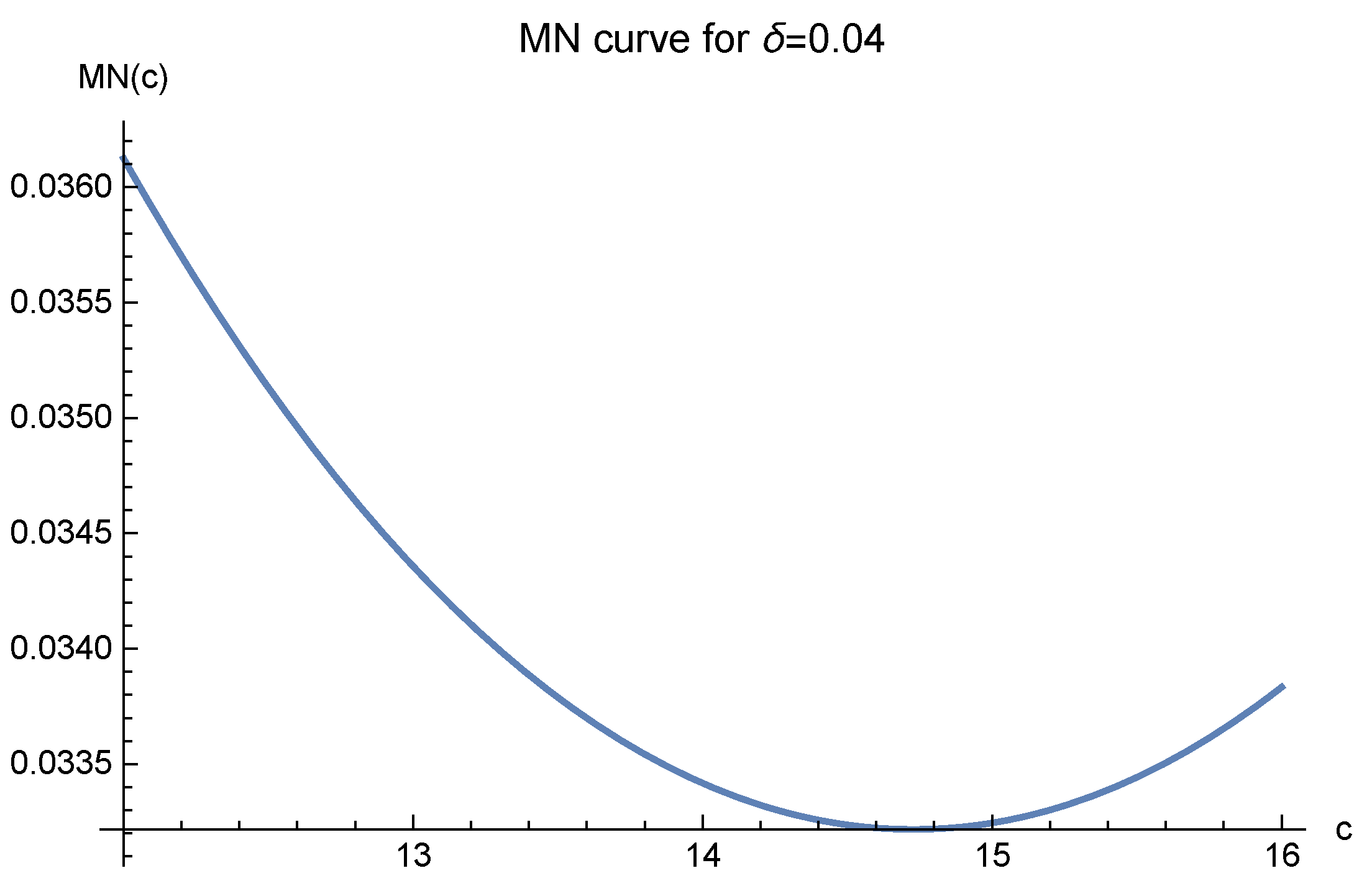
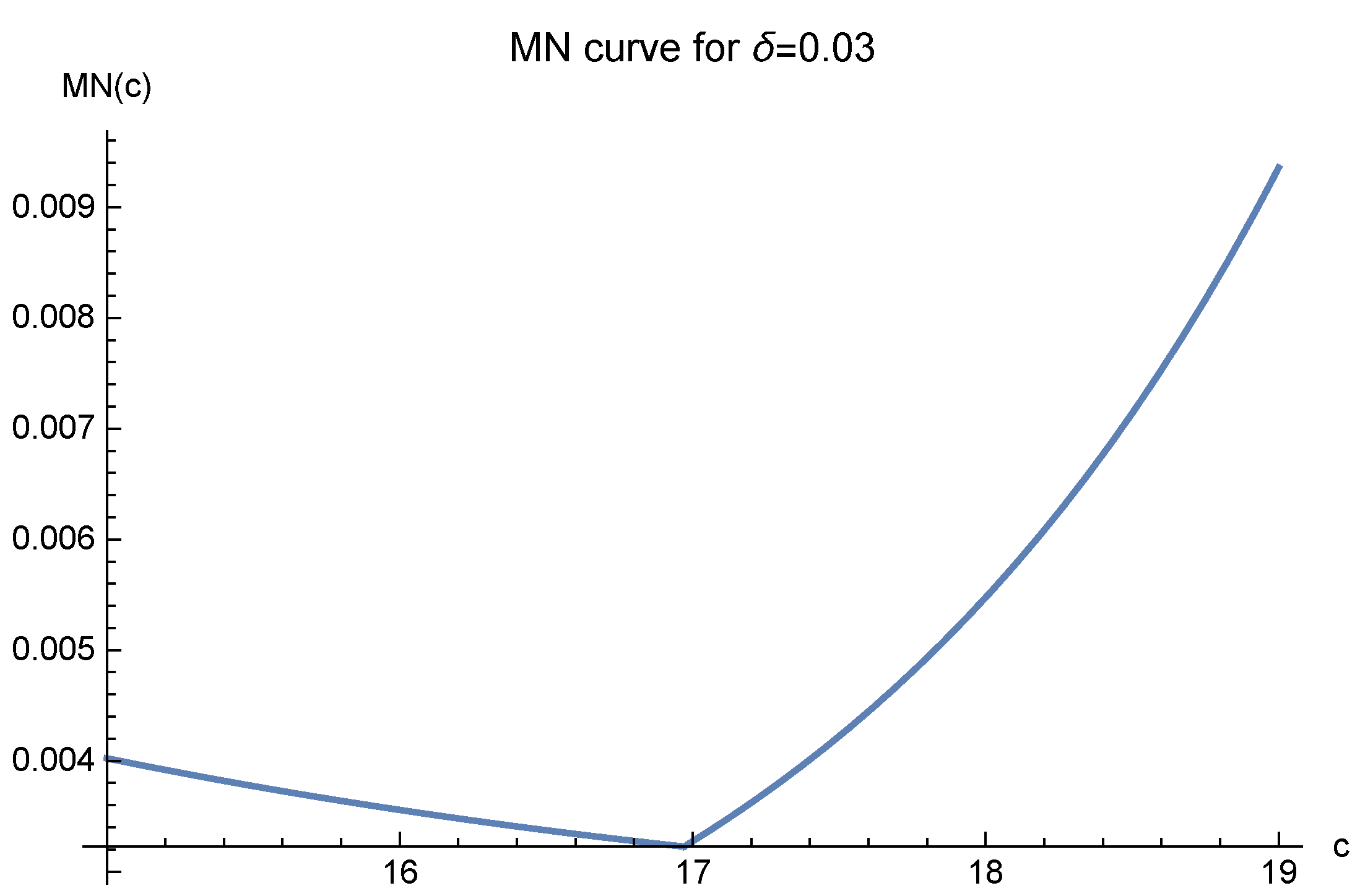
The optimal value of c minimizes the function $MN$. Although there is a restriction $c\ge c_0$, it is harmless since $c_0$ is usually very close to zero. In order to offer the reader an insight into this approach, we present in Figure 1 and Figure 2 two MN curves for Cases 1 and 2 in Luh [4]. Note that with the same fill distance $\delta$, the MN function values for $n=4$ are larger than those of $n=2$. It shows that for higher dimensions, more data points are needed in order to obtain a sharper MN curve. In fact, MN curves are very informative, as we shall see later.

2.2. The Unorthodox Approach

The reader may be frustrated by the complexity of Theorem 1 and the definition of $MN\left(c\right)$. In fact, this is not a serious issue, as will be explained in this subsection. As the inventor of this theory, the author knows that some restrictions can be relaxed, and this will greatly reduce the effort required. In Theorem 1, the parameter $b_0$ is used simply to control the size of the interpolation domain Q. Hence, one can try to let it be the diameter of the domain only. The shape of the domain is also not important. One can let it be of any shape, e.g., a cube. The parameter $\delta$ can be considered to be the widely used fill distance defined by

$$\delta =\delta (Q,X):=\underset{x\in Q}{sup}\underset{i=1,\dots ,N}{inf}\parallel x-x_i\parallel ,$$

where Q is the domain and $X=\{x_1,\dots ,x_N\}$ is the set of sample points. In fact, one can even drop the restriction of the fill distance and consider that $\delta$ is merely a positive parameter inversely proportional to the amount of data points. Then, we completely discard the severe restriction that the sample points be evenly spaced in a simplex, as defined by Definition 2. In other words, the sample points are allowed to be arbitrarily scattered in the domain. The definition of the MN functions remains unchanged as in Equations (5) and (6). All these form the so-called unorthodox approach.

In this paper, the shape parameter c is chosen by the unorthodox approach. Based on the principles introduced in Section 2.1 and the strategies introduced in this subsection, namely Section 2.2, we have a new set of criteria of choosing c, as introduced in the next two subsections.

2.3. b₀ Fixed

For $f\in E_{\sigma }$, there are two cases.

Case 1.

$\boxed{1+\lambda -n\ge 0}$For any domain of diameter $b_0>0$ and positive $\delta <\frac{b_0}{2(m+1)}$, if $1+\lambda -n\ge 0$, the optimal choice of $c\in [c_0,\infty )$ is $c^{*}\in [c_0,c_1]$, which minimizes $MN\left(c\right)$ in Equation (5) on $[c_0,c_1]$. Here, $\lambda ,n,$ and m are defined as in Equation (1).

Reason:

In this case, $MN\left(c\right)$ is increasing on $[c_1,\infty )$. Hence, its minimum value is attained in$[c_0,c_1]$.

The following case happens only when $n\ge 4$.

Case 2.

$\boxed{1+\lambda -n<0}$For any domain of diameter $b_0>0$ and positive $\delta <\frac{b_0}{2(m+1)}$, if $1+\lambda -n<0$, the optimal choice of $c\in [c_0,\infty )$ is either $c^{*}\in [c_0,c_1]$ or $c^{**}\in [c_1,\infty )$, depending on $MN\left(c^{*}\right)\le MN\left(c^{**}\right)$ or $MN\left(c^{**}\right)\le MN\left(c^{*}\right)$, where $c^{*}$ and $c^{**}$ minimize $MN\left(c\right)$ in Equation (5) on $[c_0,c_1]$ and $[c_1,\infty )$, respectively. Here, $\lambda ,n,$ and m are defined as in Equation (1).

Reason:

In this case, $MN\left(c\right)$ may not be monotonic on both $[c_0,c_1]$ and $[c_1,\infty )$.

2.4. $b_0$ Not Fixed

If the domain is unbounded and hence the sample points can be located in a bounded geometric object of arbitrarily large diameter $b_0$, then $MN\left(c\right)$ defined by Equation (6) applies. Since such $MN\left(c\right)$ is not a monotonic function, one should find $c^{*}$ that minimizes $MN\left(c\right)$ for $c\in [c_0,\infty )$ by using appropriate software, such as Mathematica or Matlab. Note that we never decrease $b_0$ because it will worsen the error bound.

3. Results

We perform a two-dimensional experiment in the unit square $\Omega =\left\{\right(x,y\left)\right|0\le x\le 1,0\le y\le 1\}$. It is shown in Madych [13] that a function $f\left(x\right)=e^{-\tilde{c}{\parallel x\parallel }^2}$ belongs to $E_{\sigma }$ if $\sigma >2\tilde{c}$. The parameter $\sigma$ greatly affects the behavior of the MN function $MN\left(c\right).$ Here, we choose $\sigma =1/10$ and $\tilde{c}=1/21$. Hence, the approximated function is $f\left(x\right)=e^{-{\parallel x\parallel }^2/21}$ for $x\in \Omega$. The radial function defined in Equation (1) is chosen to have $\lambda =2$. Thus, $m=1+\lambda /2=2$ and the interpolating function s is of the form Equation (3), where p is a two-dimensional polynomial of degree $m-1=1$. Then, we adopt the unorthodox approach to find a suitable shape parameter c.

The first step is to analyze the MN curves. The constant $\rho$ appearing in Equation (5) is only one by Definition 3, and the domain diameter $b_0$ is $\sqrt{2}$. With these understandings, we can now present the needed MN curves, as in Figure 3, Figure 4, Figure 5, Figure 6 and Figure 7.

These figures clearly show that as $\delta$ decreases, the optimal values of c move to $12b_0=16.97\approx 17$ and are fixed there. It strongly suggests that one should choose $c=17$ to make the interpolation. This method of choosing c is very reliable for the orthodox approach, as we saw in Luh [4], where the theoretically predicted optimal value coincides exactly with the experimentally optimal one. However, for the unorthodox approach, it is expected to lose some accuracy due to the removal of some severe restrictions.

In order to measure the quality of the approximation, we adopt the root-mean-square error defined by

$$RMS:=\sqrt{\sum _{i=1}^M{|f(x_i,y_i)-s(x_i,y_i)|}^2/M},$$

where $(x_i,y_i),i=1,\dots ,M,$ are test points evenly spaced in the domain $\Omega$. The number M is always chosen to be larger than the number of the randomly spaced data points (interpolating centers) N. In this section, we use $N_t$ and $N_d$ to denote M and N, respectively. We point out that the randomly spaced points are generated by the Mathematica command RandomPoint. The condition number of the interpolating matrix for establishing s is denoted by COND. As is well known, the condition number for RBF interpolation may be quite large. In order to cope with the problem of ill-conditioning, the arbitrarily precise computer software Mathematica is used. There are always enough effective digits for the calculations. For example, if COND $=1$E20, we adopt at least forty effective digits to the right of the decimal point for each step of the calculation. Hence, the results obtained are reliable. As for the crucial parameter $\delta$ contained in the MN function, we regard it as simply an indicator of the number of data points and it is inversely proportional to the data amount. When plotting the MN curves, the $\delta$s can be arbitrarily chosen, as long as their corresponding curves show clearly the trend of the optimal c values. The experimental results are presented in

Table 1. $N_d=10,N_t=441.$

c	1	17	30	50	70
RMS	$6.9\times {10}^{-4}$	$5.3\times {10}^{-4}$	$6.5\times {10}^{-4}$	$1.9\times {10}^{-4}$	$9.9\times {10}^{-5}$
COND	$4.7\times {10}^5$	$1.5\times {10}^{15}$	$6.4\times {10}^{16}$	$3.3\times {10}^{17}$	$1.8\times {10}^{17}$
c	${90}^{*}$	120	150	180	210
RMS	$6.5\times {10}^{-5}$	$1.8\times {10}^{-4}$	$1.8\times {10}^{-3}$	$2.3\times {10}^{-4}$	$2.6\times {10}^{-4}$
COND	$1.8\times {10}^{17}$	$3.4\times {10}^{17}$	$2.0\times {10}^{18}$	$3.4\times {10}^{17}$	$1.3\times {10}^{17}$

,

Table 2. $N_d=50,N_t=441.$

c	1	10*	17	30	50
RMS	$3.2\times {10}^{-6}$	$1.9\times {10}^{-7}$	$1.2\times {10}^{-6}$	$6.3\times {10}^{-5}$	$3.9\times {10}^{-5}$
COND	$9.2\times {10}^{12}$	$9.0\times {10}^{18}$	$1.0\times {10}^{19}$	$1.1\times {10}^{19}$	$7.7\times {10}^{18}$
c	70	90	120	150	180
RMS	$2.0\times {10}^{-4}$	$2.9\times {10}^{-4}$	$4.3\times {10}^{-4}$	$9.4\times {10}^{-3}$	$6.2\times {10}^{-3}$
COND	$7.5\times {10}^{19}$	$1.8\times {10}^{19}$	$5.0\times {10}^{18}$	$2.6\times {10}^{19}$	$5.0\times {10}^{19}$
c	210
RMS	$2.7\times {10}^{-3}$
COND	$2.1\times {10}^{19}$

,

Table 3. $N_d=100,N_t=441.$

c	1	10*	17	30	50
RMS	$4.4\times {10}^{-7}$	$3.7\times {10}^{-7}$	$5.6\times {10}^{-6}$	$8.1\times {10}^{-5}$	$1.1\times {10}^{-4}$
COND	$1.9\times {10}^{19}$	$4.3\times {10}^{19}$	$2.2\times {10}^{19}$	$4.4\times {10}^{19}$	$2.7\times {10}^{19}$
c	70	90	120	150	180
RMS	$1.6\times {10}^{-4}$	$1.4\times {10}^{-4}$	$6.4\times {10}^{-4}$	$1.4\times {10}^{-3}$	$2.2\times {10}^{-3}$
COND	$6.0\times {10}^{19}$	$1.8\times {10}^{19}$	$7.4\times {10}^{18}$	$2.5\times {10}^{19}$	$1.8\times {10}^{19}$
c	210
RMS	$3.7\times {10}^{-3}$
COND	$2.3\times {10}^{19}$

,

Table 4. $N_d=200,N_t=441.$

c	0.2	0.4	0.6	0.8	1
RMS	$2.8\times {10}^{-5}$	$3.4\times {10}^{-6}$	$6.7\times {10}^{-7}$	$1.7\times {10}^{-7}$	$1.3\times {10}^{-8}$
COND	$4.1\times {10}^{14}$	$8.3\times {10}^{17}$	$4.3\times {10}^{20}$	$1.3\times {10}^{20}$	$4.3\times {10}^{19}$
c	$2.2^{*}$	10	17	30	50
RMS	$3.5\times {10}^{-9}$	$8.8\times {10}^{-8}$	$1.8\times {10}^{-6}$	$1.9\times {10}^{-4}$	$1.5\times {10}^{-3}$
COND	$6.9\times {10}^{19}$	$1.4\times {10}^{20}$	$1.7\times {10}^{19}$	$2.9\times {10}^{20}$	$1.2\times {10}^{20}$
c	70	90	120	150	210
RMS	$1.6\times {10}^{-4}$	$2.1\times {10}^{-3}$	$7.2\times {10}^{-4}$	$6.0\times {10}^{-4}$	$9.9\times {10}^{-3}$
COND	$7.4\times {10}^{19}$	$4.0\times {10}^{20}$	$1.1\times {10}^{20}$	$5.5\times {10}^{19}$	$2.6\times {10}^{20}$

,

Table 5. $N_d=400,N_t=676.$

c	0.2	0.4	0.6	0.8	1
RMS	$5.4\times {10}^{-6}$	$2.2\times {10}^{-7}$	$2.8\times {10}^{-8}$	$3.1\times {10}^{-8}$	$7.1\times {10}^{-9}$
COND	$4.1\times {10}^{15}$	$1.1\times {10}^{20}$	$3.5\times {10}^{21}$	$9.0\times {10}^{20}$	$2.1\times {10}^{20}$
c	$2^{*}$	10	17	30	50
RMS	$4.1\times {10}^{-9}$	$5.7\times {10}^{-7}$	$4.7\times {10}^{-6}$	$8.4\times {10}^{-5}$	$4.2\times {10}^{-4}$
COND	$1.2\times {10}^{20}$	$7.3\times {10}^{20}$	$4.5\times {10}^{19}$	$1.0\times {10}^{20}$	$1.2\times {10}^{20}$
c	70	90	120	150	210
RMS	$1.2\times {10}^{-4}$	$5.7\times {10}^{-4}$	$8.9\times {10}^{-4}$	$3.1\times {10}^{-3}$	$9.1\times {10}^{-3}$
COND	$1.1\times {10}^{20}$	$2.4\times {10}^{20}$	$2.5\times {10}^{20}$	$4.9\times {10}^{20}$	$2.3\times {10}^{20}$

and

Table 6. $N_d=800,N_t=961.$

c	0.2	0.4	0.6	0.8	1
RMS	$3.7\times {10}^{-7}$	$1.2\times {10}^{-8}$	$1.7\times {10}^{-9}$	$6.0\times {10}^{-9}$	$1.5\times {10}^{-9}$
COND	$7.5\times {10}^{17}$	$3.6\times {10}^{21}$	$1.3\times {10}^{21}$	$8.0\times {10}^{21}$	$5.5\times {10}^{20}$
c	$4^{*}$	10	17	30	50
RMS	$1.0\times {10}^{-9}$	$5.4\times {10}^{-7}$	$2.3\times {10}^{-5}$	$2.7\times {10}^{-5}$	$1.5\times {10}^{-4}$
COND	$2.3\times {10}^{20}$	$2.2\times {10}^{22}$	$7.6\times {10}^{20}$	$3.4\times {10}^{20}$	$8.3\times {10}^{20}$
c	70	120	150	180	210
RMS	$4.4\times {10}^{-4}$	$4.5\times {10}^{-3}$	$1.4\times {10}^{-3}$	$2.3\times {10}^{-2}$	$7.4\times {10}^{-3}$
COND	$6.0\times {10}^{21}$	$2.8\times {10}^{21}$	$1.2\times {10}^{21}$	$9.7\times {10}^{20}$	$1.3\times {10}^{21}$

, where the optimal value of c is marked by the symbol ∗.

In this experiment, the most time-consuming step in solving the linear system for each c value took less than one second, even though forty effective digits were adopted for each calculation.

4. Discussion

We emphasize that our theory is reliable only when enough data points are used, and the choice of the shape parameter is determined by a series of MN curves, not only one, as stated in the third paragraph of Section 3. Moreover, our prediction may not be so accurate as in the orthodox rigorous approach of Luh [4]. These two traits can be clearly seen in these tables. However, whenever enough data points are used, our predictions are always near the experimentally optimal values and the RMSs thus obtained are satisfactory.

Note that as the number of data points increases, the RMS does seem to improve whenever the optimal c is chosen. However, if c is fixed, say $c=120$ or 210, the RMS does not improve as $N_d$ increases. This shows that increasing the number of data points is meaningful only when the shape parameter is well chosen. It may challenge the traditional concept of the convergence order based on the number of data points.

5. Conclusions

As a final conclusion, we believe that the approach presented in this paper is feasible and has greatly reduced the effort required in using the highly complicated Theorem 1 needed for the orthodox approach presented in [4]. For pure mathematicians, who insist on absolute theoretical rigor, the approach in [4] is recommended. For applied mathematicians and non-mathematicians, who emphasize practical usefulness, we strongly suggest the method presented in this paper because it is much simpler and more useful.

References

- Dyn, N. Interpolation and Approximation by Radial and Related Functions; Approximation Theory VI; Chui, C.K., Schumaker, L.L., Ward, J., Eds.; Academic Press: Cambridge, MA, USA, 1989; pp. 211–234. [Google Scholar]
- Yoon, J. Approximation in Lp(Rd) from a Space Spanned by the Scattered Shifts of a Radial Basis Function. Constr. Approx. 2001, 17, 227–247. [Google Scholar] [CrossRef]
- Yoon, J. Lp Error Estimates for `Shifted’ Surface Spline Interpolation on Sobolev Space. Math. Comput. 2003, 72, 1349–1367. [Google Scholar] [CrossRef]
- Luh, L.-T. The Shape Parameter in the Shifted Surface Spline III. Eng. Anal. Boundary Elem. 2012, 36, 1604–1617. [Google Scholar] [CrossRef]
- Abramowitz, M.; Segun, I. Handbook of Mathematical Functions. Dover Publications, Inc.: New York, NY, USA, 1970. [Google Scholar]
- Luh, L.-T. The Mystery of the Shape Parameter III. Appl. Comput. Harmon. Anal. 2016, 40, 186–199. [Google Scholar] [CrossRef]
- Wendland, H. Scattered Data Approximation; Cambridge University Press: Cambridge, UK, 2005. [Google Scholar]
- Buhmann, M. Radial Basis Functions: Theory and Implementations; Cambridge University Press: Cambridge, UK, 2003. [Google Scholar]
- Fleming, W. Functions of Several Variables, 2nd ed.; Springer: Berlin/Heidelberg, Germany, 1977. [Google Scholar]
- Luh, L.-T. The Equivalence Theory of Native Spaces. Approx. Theory Appl. 2001, 17, 76–96. [Google Scholar]
- Madych, W.R.; Nelson, S.A. Multivariate Interpolation and Conditionally Positive Definite Function. Approx. Theory Appl. 1988, 4, 77–89. [Google Scholar] [CrossRef]
- Madych, W.R.; Nelson, S.A. Multivariate Interpolation and Conditionally Positive Definite Function, II. Math. Comp. 1988, 54, 211–230. [Google Scholar] [CrossRef]
- Madych, W.R. Miscellaneous Error Bounds for Multiquadric and Related Interpolators. Comp. Math. Appl. 1992, 24, 121–138. [Google Scholar] [CrossRef] [Green Version]