Article

Multigrid Method for Solving Inverse Problems for Heat Equation

1
Department of System Programming, South Ural State University, 454080 Chelyabinsk, Russia
2
Ministry of Electricity, The State Company Electricity Production, Baghdad 10053, Iraq
3
Faculty of Science, School of Science and Technology, University of New England, Armidale, NSW 2350, Australia
4
Department of Food and Biotechnology, South Ural State University, 454080 Chelyabinsk, Russia
*
Author to whom correspondence should be addressed.
Mathematics 2022, 10(15), 2802; https://doi.org/10.3390/math10152802
Submission received: 16 July 2022 / Revised: 3 August 2022 / Accepted: 5 August 2022 / Published: 7 August 2022
(This article belongs to the Section Computational and Applied Mathematics)

Abstract

:
In this paper, the inverse problems for the boundary value and initial value in a heat equation are posed and solved. It is well known that those problems are ill posed. The problems are reformulated as integral equations of the first kind by using the separation-of-variables method. The discretization of the integral equation allowed us to reduce the integral equation to a system of linear algebraic equations or a linear operator equation of the first kind on Hilbert spaces. The Landweber-type iterative method was used in order to find an approximation solution. The V-cycle multigrid method is used to obtain more frequent and fast convergence for iteration. The numerical computation examples are presented to verify the accuracy and fast computing of the approximation solution.
MSC:
35-00; 35-01; 35-02; 35-03; 35-04; 35-06; 35-11

1. Introduction

In the early twentieth century, Hadamard [1] labeled some well-posed problems, stating that a problem is well posed when it fulfills the following points:
  • Solution exists.
  • Uniqueness—this solution is unique.
  • Stability (the given data are continuously dependent on the solution).
If at least one of the above points or conditions is not fulfilled, the problem is considered an ill-posed problem. The violations of 1 and 2 can often be improved with a small re-formulation of the problem. Violations of stability are much harder to remedy because they imply that a small disturbance in the data leads to a large disturbance in the estimated solution [2,3,4,5].
The inverse problem under the study of the heat equation can be solved by many methods. For example, the method of regularization Tikhonov A.N. [6], by the method of Lavrentiev M.M. [7], by the method of quasi-solutions Ivanov V.K. [8] and many others. Various methods and algorithms for solving IP “inverse problems” were explained and used in [9,10,11,12,13,14,15,16,17,18,19]. The success of these methods and algorithms is largely based on understanding and analyzing the mathematical problems related to the declarations of the properties in these IP “inverse problems” and identifying specific difficulties in solving them [20,21,22,23,24,25].
One of the many known methods of solving a linear operator equation is the iteration method, such us the Landweber iteration method. This method has several issues, such as initial guess, complexity, and convergence. The discretization process for the integral equation primes to a huge, sparse, and highly structured system of linear equations or linear operator equations. Inappropriately, theoretic convergence studies and mathematical experiments show that the convergence rate is slow for these iterative algorithms, leading to an amplified cost of iteration [26]. The direct iteration method suffers from some restricting boundaries. Multigrid methods advanced from efforts to overcome these limitations. Multigrid settings are largely successful when used with relaxation or iteration methods and they lead to fast and direct point-to-estimated solutions to solve the IP “inverse problems”.
Multigrid methods [27,28,29,30] are often used to accelerate the convergence rate of iterative or relaxing methods. This is an effective method for solving large systems of linear algebra equations, which results from the discretization of integral equations or PDE. Multigrid methods have been applied to least-squares wave front reconstruction [31]. This method has also been used to solve inverse problems with linear parabolic PDE constraints [32] and ODT problems [29].
In this work, we provide a new algorithm for numerical solutions to the integral equations of the first kind by using the V-cycle multigrid method and comparing it with the Landweber iteration method. In this article, we mixed between the Landweber iteration method and the multigrid method to obtain accelerated solutions
We consider the following two forms of the integral equation of the first kind that come from two inverse ill-posed heat equation problems.
A u ( t ) = a b K ( t , x ) u ( t ) d x = f ( t )
where t [ c , d ] and the kernel K ( x , t ) , K t ( x , t ) C ( [ a , b ] × [ c , d ] ) , and f ( t ) L 2 [ c , d ] , the (1) can represent the initial value problem for heat equation.
A u ( t ) = 0 t K ( t , τ ) u ( τ ) d τ = f ( t )
where t [ 0 , T ] and K ( t , τ ) corresponding the kernel function for the integral Equation (2), K ( t , τ ) , K t ( t , τ ) , K t ( t , τ ) C ( [ a , b ] × [ 0 , T ] ) ,   u ( t ) L 2 [ 0 , T ] . This type of integral equation can represent the boundary value problem for the heat equation.
Problems (1) and (2) can be reduced to the form of the leaner operator equation after applying the discretization algorithm.
A u = f
The solution vector u R n should reduce the following minimizing problem.
min u R n | | A u f | | 2
where A R n × n is a large matrix and the vector f R n represents known error-contaminated data and can be expressed as the following.
f = f t r u e + η
where f t r u e is an unknown error-free vector associated with f and η represents the error in f . The noise may stem from measurement and/or discretization errors.
| | η | | δ
where δ is given and known as error level.
The approaches proposed in this work are the Landweber-type iterative method to obtain a good approximation solution for (3). Then, the multigrid method was used to obtain a more complete and fast solution by using the Landweber type as relaxation iterative in post-smoothing and pre-smoothing parts.
All these steps are organized through the sections in this paper. Section 2 defines the linear partial differential equations and describes the solution as an integral equation of the first kind for the boundary value problem and the initial value problem of the heat equation. Section 3 describes the general notations and the iterative Landweber-type method. Section 4 describes and implements the V-cycle multigrid method. After that, in Section 5, the numerical examples are presented to explain our analysis. Finally, the explanation of the suggested method is summarized in Section 6.

2. Problem Statement

In this section, we briefly present two-class problems: the boundary value and initial value problems. Both problems can be reduced to an integral equation by using the separation-of-variables method. Then, by implementing the discretization process, we obtain the linear operator equation. The inverse ill-posed problems have been studied and solved in many works with a different method [11,12,13,14].

2.1. Inverse Boundary Value Problem

We consider the inverse boundary value problem given in [33,34] with time interval [ 0 , T ] .
u ( x , t ) t = 2 u ( x , t ) x 2 ; x ( 0 , x ) , t ( 0 , T ]
u ( x , 0 ) = 0 ;       x [ 0 , 1 ]
u ( 0 , t ) x = 0 ;     t ( 0 , T ]
u ( 1 , t ) = u ( t ) ;       t ( 0 , T ]
suppose that the u ( t ) H 4 [ 0 , T ] , is a function such that
u ( 0 ) = u ( 0 ) = u ( 0 ) = u ( T ) = u ( T ) = 0
where 0 T | u ( t ) | 2 d t r 2 ,     r known number. By using the separation-of-variables method, we obtained the following solution.
u ( x 0 , t ) = n = 0 C n ( t ) cos ( ( n + 0.5 ) π x 0 ) + u ( t )
where the x 0 ( 0 , 1 ) , t [ 0 , T ]
C n ( t ) = 2 e ( n + 0.5 ) 2 π 2 t ( n + 0.5 ) π 0 t u ( τ ) e ( n + 0.5 ) 2 π 2 τ d τ
integrating by parts the right-hand side of Formula (13) twice, we obtain
C n ( t ) = 2 ( n + 0.5 ) π 0 t u ( τ ) e ( n + 0.5 ) 2 π 2 ( t τ ) d τ + 2 ( n + 0.5 ) 3 π 3 u ( t ) [ 2 ( n + 0.5 ) 3 π 3 u ( 0 ) + 2 ( n + 0.5 ) 5 π 5 u ( t ) + 2 ( n + 0.5 ) 5 π 5 u ( 0 ) ]
C n ( t ) = 2 ( n + 0.5 ) 5 π 5 0 t u ( τ ) e ( n + 0.5 ) 2 π 2 ( t τ ) d τ [ 2 ( n + 0.5 ) 3 π 3 u ( 0 ) + 2 ( n + 0.5 ) 5 π 5 u ( 0 ) ]
where u ( 0 ) = u ( 0 ) = 0 by (11)
C n ( t ) = 2 ( n + 0.5 ) 5 π 5 0 t u ( τ ) e ( n + 0.5 ) 2 π 2 ( t τ ) d τ
From (12) and (16) we have the following integral equation of the first kind
f ( t ) = u ( x 0 , t ) = 0 t [ u ( t ) + n = 0 2 cos ( n + 0.5 ) π x 0 ( n + 0.5 ) 5 π 5 e ( n + 0.5 ) 2 π 2 ( t τ ) ] g ( τ ) d τ
where u ( τ ) = g ( τ ) . We need to define an operator B : L 2 [ a , b ] L 2 [ a , b ] by the following formula.
B g ( τ ) = u ( t ) = 0 t ( t τ ) 2 2 g ( τ ) d τ
where B g ( τ ) L 2 [ 0 , T ] .
We used the algorithm in [6] with a specified derivative term for the kernel and obtained the following.
A u ( t ) = 0 t K ( t , τ ) g ( τ ) d τ = f ( t )
where t [ 0 , T ] .
Where A is finite-dimensional operator. For the next step, we need to apply the discretization algorithm [5,6] on the integral Equation (19)
K ¯ i ( t ) = K ( t , τ i )
K ¯ i ( t ) ; τ i τ τ i + 1 ,   t [ 0 , T ] , i = 0 , 1 , , n 1
K ¯ i ( t j ) ; τ i τ τ i + 1 , t j t t j + 1 , i = 0 , 1 , , n 1 , j = 0 , 1 , , n 1
K n ( t , τ ) = K ¯ i ( t j )
A [ u ( t ) ] = 0 t K n ( t , τ ) g ( τ ) d τ = f ( t ) , t [ 0 , T ]
the value of kernel depended on the following condition.
K ¯ i ( t j ) = { K ( t j , τ i )           i j 0 ?                                   i > j
From above, we convert the boundary value problem to linear operator equation A u = f , where u = B g , by reducing the integral equation to a system of linear algebra equations.
A B [ g ( τ 0 ) g ( τ 1 ) g ( τ n 1 ) ] = [ f ( t 0 ) f ( t 2 ) f ( t n 1 ) ]
where
A = 1 n [ K ( τ 0 , t 0 ) 0 K ( τ 0 , t 1 ) K ( τ 1 , t 1 ) 0 0 K ( τ 0 , t n 1 ) K ( τ 1 , t n 1 ) K ( τ n 1 , t n 1 ) ]
The operator A in (27) is a triangular operator.

2.2. Initial Value Problem

The second inverse problem is the initial value problem for the heat equation has been described by the following linear partial differential equation.
u ( x , t ) t = 2 u ( x , t ) x 2   , x [ 0 , l ] , t ( 0 , T ]
u ( 0 , t ) = 0 , t ( 0 , T ]
u ( l , t ) = 0 , t ( 0 , T ]
u ( x , 0 ) = u ( x ) , x [ 0 , l ]
where u ( 0 , t ) and u ( l , t ) are boundary conditions, u 0 ( x ) is an initial condition, which needs to be found. This problem was solved in [35] by using Tikhonov’s regularization inversion method and it was solved by Picard’s method in [2]. In this work, we apply another numerical algorithm to obtain a more accurate solution and fast implementation with a high-scale problem. The integral form for this equation will be
A u ( x ) = 0 l K ( x , y ) u ( y ) d y = f ( x )
where the kernel K ( x , y ) is an infinite series and we cannot handle the infinite sum, so we need to make the sum of series finite to 10-times
K ( x , y ) = 2 l n = 1 10 e ( n π ) 2 T l 2 sin ( n π x l ) sin ( n π y l ) ,     T > 0
For giving the approximate solution to u ( x ) , we can rewrite the problem as linear algebraic equations where the form will be A u = f .
A [ u ( y 0 ) u ( y 2 ) u ( y n 1 ) ] = [ f ( x 0 ) f ( x 2 ) f ( x n 1 ) ]
where
A = l 0 n [ K ( x 0 , y 0 ) K ( x 0 , y 1 ) K ( x 0 , y n 1 ) K ( x 1 , y 0 ) K ( x 1 , y 1 ) K ( x 1 , y n 1 ) K ( x n 1 , y 0 ) K ( x n 1 , y 1 ) K ( x n 1 , y n 1 ) ]
The bounded operator A is ill conditioned and any numerical attempt to directly solve (35) will fail.

3. Iterative Method

We first establish the notations for the linear operator Equation (3). We used the vector u to denote the true solution and used the vector v to denote the estimate solution; perhaps v is generated by the iterative method. There are two significant measures; the first one is the error vector e ,
e = u v
Unfortunately, the error is unknown because the vector u is not given. The second measure is residual r , defining how well v approximates u ; it is given by
r = f A v
The residual is simply the amount by which the approximation v fails to satisfy the original problem (3). There is an equation defining the relationship between the error e and residual r
e = A r
In order to improve the estimation of the vector v , we solve Equation (38). After that, we compute the new estimation by using the definition of the error equation
u = e + v

Landweber-Type Method

The Landweber-type iteration method will be used in this work.
v k + 1 = v k + λ k A T M ( f A v k ) , k = 0 , 1 , ,
where λ k is the relaxation parameter and M is the symmetric positive definite operator. We used the classical Landweber method, where the operator M is defined as identity matrix [36]. The Landweber-type method has a self-regularization property. This property is very important to reduce the errors in the regularized solution by controlling the mechanism of convergence. In order to enhance convergence, we need to select λ k relaxation parameter. In [37], there is an important theorem, which proves how the value of the relaxation parameter make iterations of (40) converge to a solution of min u R n | | A u f | | 2 .
Theorem 1.
Let λ k = λ for k 0 . Then, the iterates of (40) converge to a solution ( v ) of (3) if and only if 0 < λ < 2 / σ 1 2 with σ 1 the largest singular value of M A . If, in addition, v 0 R ( A T ) then v is the unique solution with minimal norm.
This theorem was proved in [37] with a constant relaxation parameter λ k = λ . To reduce error in the iterative method (40), the following relaxation parameters are studied by [38]:
λ k = | | w k | | 2 | | M A r k | | 2
where r k = f A v k and w k = A T M r k for k = 0 , 1 , .
The following Algorithm 1 explains how to write the program code for the Landweber-type iteration method with a variable relaxation parameter.
Algorithm 1 L.T.1
For loop: k: =1, 2, 3,…
n = s i z e ( u , 1 ) ; % determine the size of domain
v = z e r o s ( n 1 , 1 ) ; % initial guess (zeros vector)
M = o n e ( n 1 , n 1 ) ; % create Identity Matrix
r = f ( A v k ) ; w = A T I r ; λ = | | w | | 2 | | I A r | | 2 ; v = v + ( λ A T M ) ( f A v ) ;
End loop
The next Algorithm 2 explains the Landweber-type iteration method with a constant relaxation parameter.
Algorithm 2 L.T.2
For loop: k: =1, 2, 3,…
n = s i z e ( u , 1 ) ; % determine the size of domain
v = z e r o s ( n 1 , 1 ) ; % initial guess (zeros vector)
M = o n e ( n 1 , n 1 ) ; % create Identity Matrix
λ = n u m b e r ; % determine the relaxation parameter
v = v + ( λ A T M ) ( f A v ) ;
End loop
Those algorithms can be used in next section as a relax function.

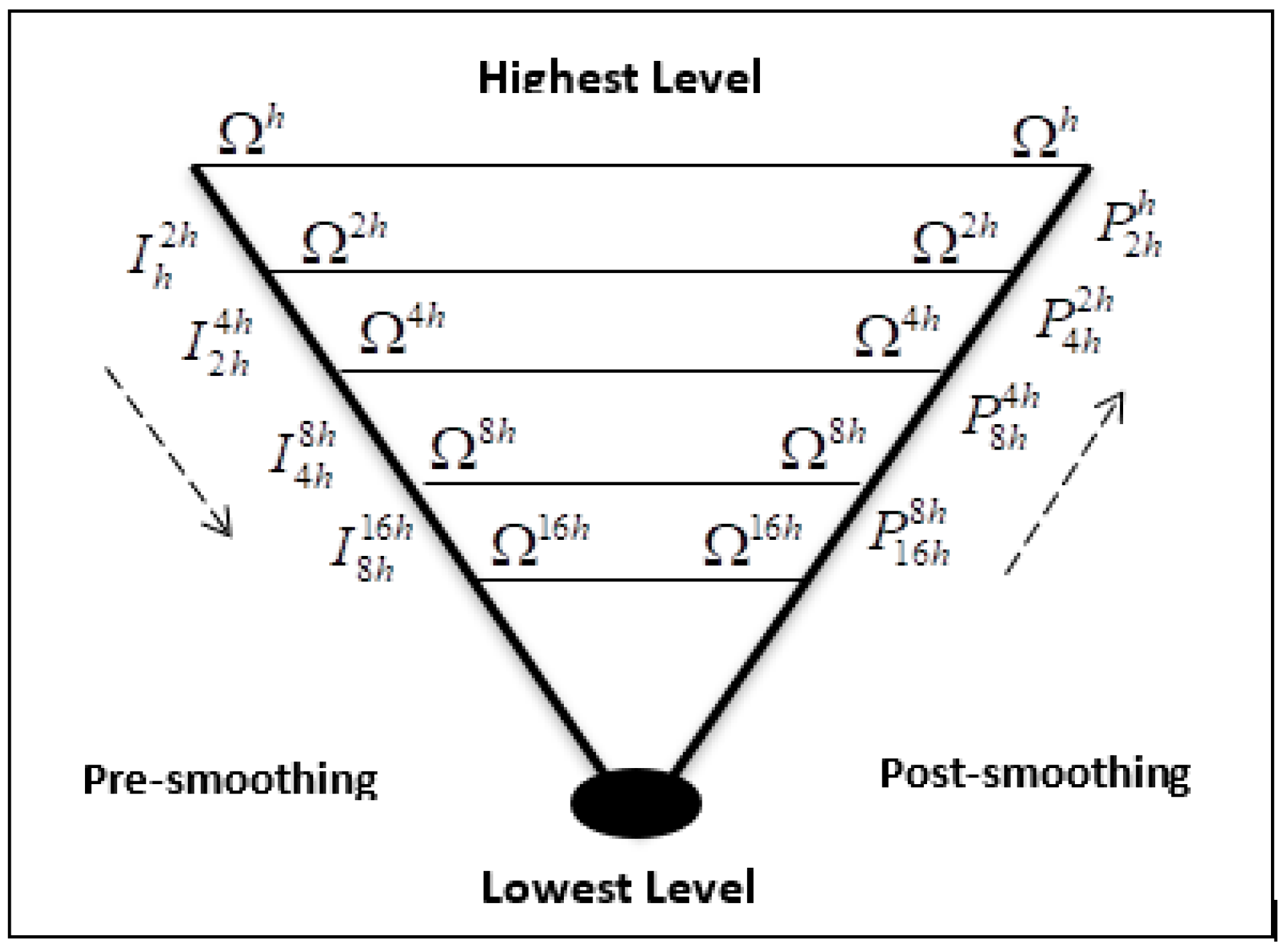
4. Multigrid Method Algorithms

The goal of the multigrid method is to recover the limitations in the iteration method, at least in its primary stages, by using a good initial guess. A well-known technique for obtaining an enhanced initial guess is by performing some preliminary iterations on a coarse grid. Iterations on a coarse grid are less expensive because there are fewer unknowns to be updated. We noted the grid name as with points. Add the new notations to (3).
A h u h = f h ,   on   Ω h
the coarse grid Ω 2 h with ( n 2 1 ) points noted as
A 2 h u 2 h = f 2 h . on   Ω 2 h
The multigrid method consists of two main steps. One is the smoothing operators and the other is the grid transfer operators. We used the Landweber method as a smoothing method in the algorithm. We named this step “relaxing”. In the grid transfer operator step, we have two types of operators: the prolongation and the interpolation operator. We used a simple method to define those operators, which is explained in [30]. The prolongation operator P takes the vector in a coarse grid and produces the fine-grid vector P 2 h h : Ω 2 h Ω h . The interpolation operator I transfer a vector from a fine grid to a coarse grid I h 2 h : Ω h Ω 2 h as shown in Figure 1.
The prolongation operator P 2 h h : Ω 2 h Ω h according to the rule P 2 h h v 2 h = v h , where
v 2 j h = v j 2 h
v 2 j + 1 h = 1 2 ( v j 2 h + v j + 1 2 h ) , 0 j n 2 1
It is clear that the P 2 h h operator is mapping from R n 2 1 to R n 1 . It has full-rank null space N = { 0 } . This operator has the general form
P 2 h h v 2 h = 1 2 [ 1 2 1 1 2 1 1 2 1 1 2 1 ] ( n 1 ) × ( n 2 1 ) [ v 1 v 2 v n 2 1 ] = [ v 1 v 2 v 3 v n 1 ] = v h
The interpolation operator I h 2 h is mapping R n 1 to R n 2 1 ,
I h 2 h v h = 1 4 [ 1 2 1 1 2 1 1 2 1 1 2 1 ] ( n 2 1 ) × ( n 1 ) [ v 1 v 2 v 3 v n 1 ] = [ v 1 v 2 v n 2 1 ] = v 2 h
In this work, we will use the V-cycle multigrid method. There are two smoothing parts: the pre-smooth and the post-smooth. We need to apply relax (iterative computing method) to each node to obtain a solution vector. We transfer the vector from fine grid to coarse grid by using an interpolation operator I in the pre-smoothing part. In the post-smoothing part, the vector transfers from coarse grid to fine grid by using the prolongation operator P , see Figure 2.
If we apply the V-cycle method twice, we get a W-cycle multigrid. The relax action was implemented by a Landweber-type iteration (40). The relax action reduces the high frequency of error and the result of the relax stage is noted as vector v L h , L = 1 , 2 , 4 , 8 , 16 , 32 , 64 , 128 , .
Pre-smoothing
  • Relax A h u h = f , initial guess v h = 0
  • Compute residual r 2 h = I h 2 h r h , r h = f h A h v h
  • Relax A 2 h e 2 h = r 2 h , initial guess v 2 h = 0
  • Compute residual r ^ 4 h = I 2 h 4 h r ^ 2 h , r ^ 2 h = r 2 h A 2 h v 2 h
  • Relax A 4 h e 4 h = r ^ 4 h , initial guess v 4 h = 0
  • Compute residual r 8 h = I 4 h 8 h r 4 h , r 4 h = r ^ 4 h A 4 h v 4 h
Lowest Level
  • Solve A L h e L h = r L h
Post-smoothing
  • correct v 4 h v 4 h + P 8 h 4 h v 8 h
  • Relax A 4 h e 4 h = r ^ 4 h , initial guess v 4 h
  • correct v 2 h v 2 h + P 4 h 2 h v 4 h
  • Relax A 2 h e 2 h = r 2 h , initial guess v 2 h
  • correct v h v h + P 2 h h v 2 h
  • Relax A h u h = f , initial guess v h
    where A 2 h = I h 2 h A h P 2 h h and A 4 h = I 2 h 4 h A 2 h P 4 h 2 h .

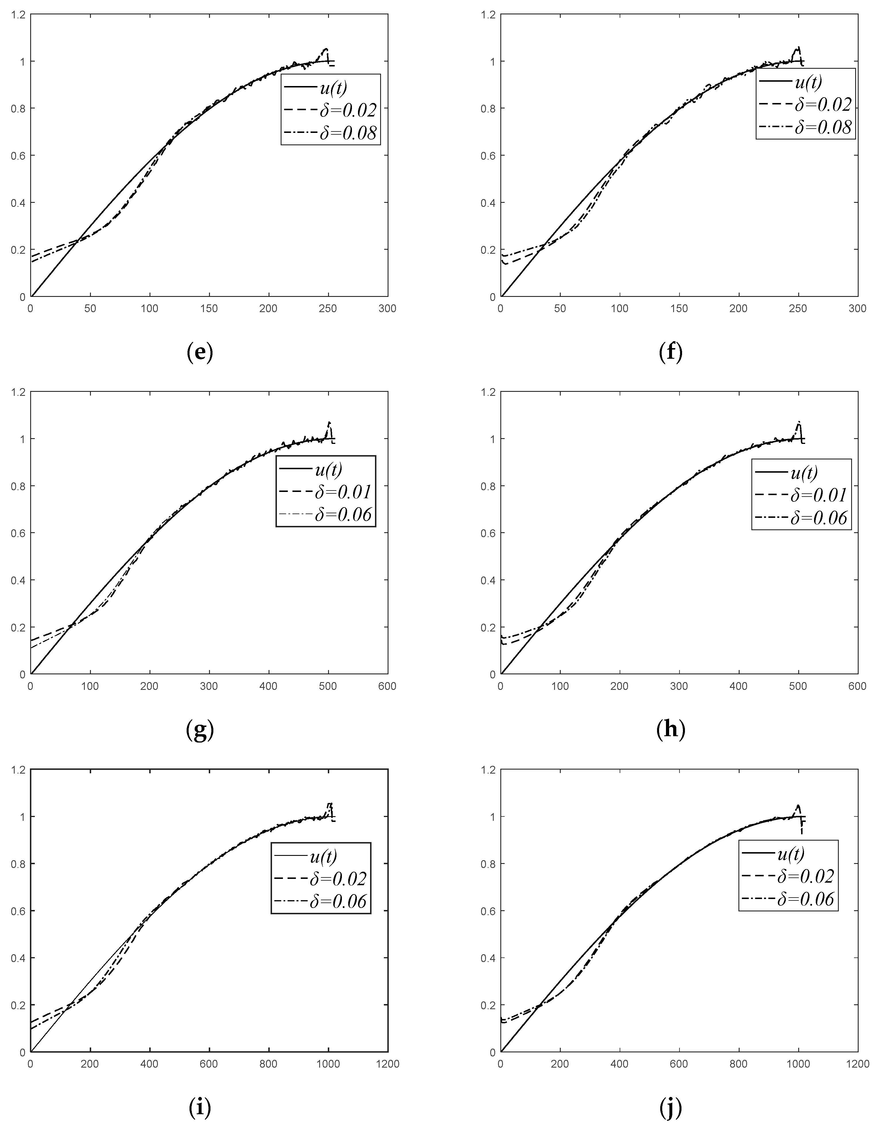
5. Numerical Results

We will compare between the Landweber-type method and V-cycle multigrid method by considering the time and error level.

5.1. Boundary Value Problem

Considering the inverse boundary value problem (7)–(11) for the heat equation, we need to find   u ( t ) H 4 [ 0 , T ] . The exact solution will be   u ( t ) , and the input function for inverse problem   u ( x 0 , t ) = f ( t ) , where the x 0 ( 0 , 1 ) , t   [ 0 ,   T ] , x 0 = 0.5 and T = 5 , as shown in Figure 3.
We tested the two algorithms in different domains Ω h with different noise levels. The results are shown in Table 1. When we called the Call Algorithm 1 L.T.1 or Algorithm 3 V.M algorithm, we used Call Algorithm 1 L.T.1 or Algorithm 1 L.T.1 in Relax ( A v = f ) step with 100 iterations.
Algorithm 3 V.M
g r i d ( A , v , f )    % define function grid with three input
n = s i z e ( v , 1 ) ; % determine the size of domain
Relax   ( A v = f ) % Call Algorithm 1 L.T.1 or Algorithm 2 L.T.2 with low iteration times
If (n > size of lowest level)
r = f A v ; % Compute Residual
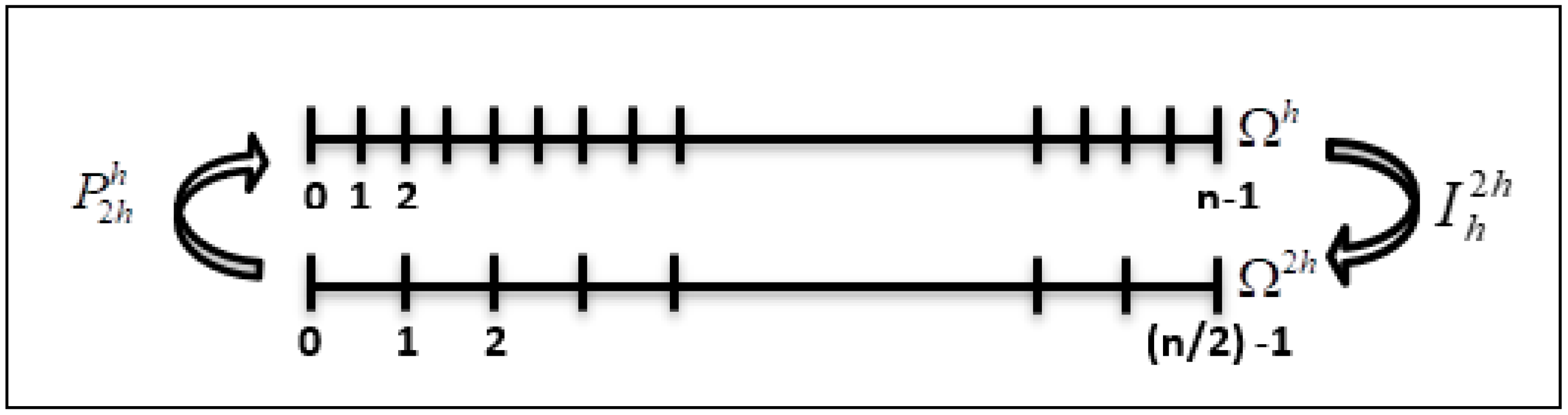
for i = 1:n % Create prolongation matrix
P(2*i − 1, i) = 1;
P(2*i, i)= 2;
P(2*i + 1, i) = 1;
End
I = P T ; % Create interpolation matrix
r _ t o _ c = 0.25 * I r ; % from fine-grid to coarse-grid
A _ n = 0.25 * I * A * 0.5 * P ;   % Create   A L h interpolation matrix
v = z e r o s ( size ( r _ t o _ c , 1 ) , 1 ) ; % initial guess (zeros vector)
e _ t o _ c = g r i d ( A _ n , v , r _ t o _ c ) ; % used recursion function
e = 0.5 * P * e _ t o _ c ; %from coarse-grid to fine-grid
v = v + e ; % correct
end
Relax   ( A v = f ) % Call Algorithm 1 L.T.1 or Algorithm 2 L.T.2 with low iteration times with low iteration times
o u t p u t = v ;
E n d _ g r i d ;
The above table shows the Algorithm 3 V.M has speeded the computation time compared with the L.T.1 algorithm. The solutions for two algorithms in Ω h are shown in Figure 4.

5.2. Initial Value Problem

Considering the inverse initial value problem (28)–(31) for the heat equation, we need to find u ( x ) L 2 [ 0 , 1 ] . The exact solution will be u ( x ) = sin π x , 0 x 1 . We created the input function for the inverse problem, as shown in Figure 5. u ( x , T ) = f ( x ) , 0 x 1 and T = 0.01 .
In this numerical example, we will use the Landweber-type method with constant relaxation parameter λ k = λ ; also, we will use the same iterative method in V-cycle multigrid with constant relaxation parameter. We compared the two algorithms with a high scale of domains Ω h . The results are shown in Table 2. When we called the V.M. algorithm, we used L.T.1 in Relax ( A v = f ) step with 10 iterations.
From the above results, we see the Algorithm 3 V.M Algorithm successfully applied to obtain a good approximating solution with low time in high-scale domains Ω h , see Figure 6.

6. Conclusions

This work deals with algorithms for solving the boundary value problem and the initial value problem for the heat equation and some results were collected. The forward problem was solved by the separation-of-variables method and then the PED is converted to an integral equation of the first kind. By using the discretization method, we converted the integral equation to a linear operator equation for the first kind. The Landweber iteration method was successfully applied to obtain an estimated solution. The V-cycle multigrid method is applied to make the computation cost for the iterative method cheap and more accurate. It is clear that the V.M. algorithm has a recursion function, named grid. W used a low number of iterations in each relaxing step inside the grid function. The results show the CPU time for solving each equation in a specific domain size is accelerated by using a low iteration number in grid function through all the low domains in V.M. algorithm. All results in this numerical example show that the multigrid method is fast, more convergent and accurate. In future work, parallel computing will be used to make the cost of computing cheaper.

Author Contributions

Data curation, H.K.I.A.-M., M.A., H.A. and A.-M.Z.T.; formal analysis, M.A., H.A., A.B. and A.K.; funding acquisition, H.A.; investigation, H.K.I.A.-M., M.A. and H.A.; methodology, H.K.I.A.-M., M.A., A.-M.Z.T. and A.B.; project administration, M.A., H.A. and A.B.; resources, A.-M.Z.T. and A.K.; software, H.K.I.A.-M. and M.A.; visualization, M.A. All authors have read and agreed to the published version of the manuscript.

Funding

The work was supported by Act 211 Government of the Russian Federation, contract No. 02.A03.21.0011. The work was supported by the Ministry of Science and Higher Education of the Russian Federation (government order FENU-2020-0022).

Conflicts of Interest

The authors declare no conflict of interest.

References

  1. Daniell, P.J.; Hadamard, J. Lectures on Cauchy’s Problem in Linear Partial Differential Equations. Math. Gaz. 1924, 12, 173–174. [Google Scholar] [CrossRef]
  2. Al-Mahdawi, H.K. Studying the Picard’s Method for Solving the Inverse Cauchy Problem for Heat Conductivity Equations. Bull. South Ural State Univ. Ser. Comput. Math. Softw. Eng. 2019, 8, 5–14. [Google Scholar] [CrossRef]
  3. Al-Mahdawi, H.K. Development the Regularization Computing Method for Solving Boundary Value Problem to Heat Equation in the Composite Materials. J. Phys. Conf. Ser. 2021, 1999, 012136. [Google Scholar] [CrossRef]
  4. Al-Mahdawi, H.K. Development the Numerical Method to Solve the Inverse Initial Value Problem for the Thermal Conductivity Equation of Composite Materials. J. Phys. Conf. Ser. 2021, 1879, 032016. [Google Scholar] [CrossRef]
  5. Al-Mahdawi, H.K.; Sidikova, A.I. An approximate solution of fredholm integral equation of the first kind by the regularization method with parallel computing. Turk. J. Comput. Math. Educ. 2021, 12, 4582–4591. [Google Scholar]
  6. Tikhonov, A.N. On the regularization of ill-posed problems. Proc. USSR Acad. Sci. 1963, 153, 49–52. [Google Scholar]
  7. Lavrentiev, M.M. The inverse-problem in potential theory. Dokl. Akad. Nauk. SSSR 1956, 106, 389–390. [Google Scholar]
  8. Ivanov, V.K. The application of Picard’s method to the solution of integral equations of the first kind. Bull. Inst. Politenn. Iasi. 1968, 14, 71–78. [Google Scholar]
  9. Tanana, V. Completeness of the system of eigenfunctions of the Sturm-Liouville problem with the singularity. Vestn. Udmurt. Univ. Mat. Mekhanika. Komp’yuternye Nauk. 2020, 30, 59–63. [Google Scholar] [CrossRef] [Green Version]
  10. Tanana, V.P.; Sidikova, A.I. Optimal Methods for Ill-Posed Problems: With Applications to Heat Conduction; Walter de Gruyter GmbH & Co. KG: Berlin, Germany, 2018; Volume 62. [Google Scholar]
  11. Tanana, V.P. Optimization of Methods for Solving Inverse Problems. In Proceedings of the 2018 International Russian Automation Conference (RusAutoCon), Chelyabinsk, Russia, 9–16 September 2018; pp. 1–7. [Google Scholar]
  12. Tanana, V.P.; Markov, B.A. The control problem for the heat equation in the case of a composite material. J. Phys. Conf. Ser. 2021, 1715, 012049. [Google Scholar] [CrossRef]
  13. Tanana, V.P.; Sidikova, A.I.; Ershova, A.A. A numerical solution to a problem of crystal energy spectrum determination by the heat capacity dependent on a temperature. Eurasian J. Math. Comput. Appl. 2017, 5, 87–94. [Google Scholar] [CrossRef]
  14. Tanana, V.P.; Rudakova, T.N. The optimum of the MM Lavrent’ev method. J. Inverse Ill-Posed Probl. 2011, 18. [Google Scholar] [CrossRef]
  15. Ivanov, V.K.; Vasin, V.V.; Tanana, V.P. Theory of Linear Ill-Posed Problems and Its Applications; Walter de Gruyter: Berlin, Germany, 2013; Volume 36. [Google Scholar]
  16. Tanana, V.P. A comparison of error estimates at a point and on a set when solving ill-posed problems. J. Inverse Ill-Posed Probl. 2017, 26, 541–550. [Google Scholar] [CrossRef]
  17. Tanana, V.P. On Reducing an Inverse Boundary-Value Problem to the Synthesis of Two Ill-Posed Problems and Their Solution. Numer. Anal. Appl. 2020, 13, 180–192. [Google Scholar] [CrossRef]
  18. Tanana, V.P.; Vishnyakov, E.Y.; Sidikova, A.I. An approximate solution of a Fredholm integral equation of the first kind by the residual method. Numer. Anal. Appl. 2016, 9, 74–81. [Google Scholar] [CrossRef]
  19. Tanana, V.P.; Markov, B.A. Uniqueness, existence and solution of the direct boundary heat exchange problem for a weakly non-linear temperature conductivity coefficient. J. Phys. Conf. Ser. 2021, 1715, 012050. [Google Scholar] [CrossRef]
  20. Glasko, V.B.; Kulik, N.I.; Shklyarov, I.N.; Tikhonov, A.N. An inverse problem of heat conductivity. Zhurnal Vychislitel’Noi Mat. I. Mat. Fiz. 1979, 19, 768–774. [Google Scholar]
  21. Belonosov, A.S.; Shishlenin, M.A. Continuation problem for the parabolic equation with the data on the part of the boundary. Siber. Electron. Math. Rep. 2014, 11, 22–34. [Google Scholar]
  22. Kabanikhin, S.I.; Hasanov, A.; Penenko, A.V. A gradient descent method for solving an inverse coefficient heat conduction problem. Numer. Anal. Appl. 2008, 1, 34–45. [Google Scholar] [CrossRef]
  23. Yagola, A.G.; Stepanova, I.E.; Van, Y.; Titarenko, V.N. Obratnye zadachi i metody ikh resheniya. Prilozheniya k geofizike. In Inverse Problems and Methods for their Solution: Applications to Geophysic; Binom. Laboratoriya Znanii: Moscow, Russia, 2014. [Google Scholar]
  24. Kabanikhin, S.I.; Krivorot’Ko, O.I.; Shishlenin, M.A. A numerical method for solving an inverse thermoacoustic problem. Numer. Anal. Appl. 2013, 6, 34–39. [Google Scholar] [CrossRef]
  25. Tanana, V.P. On the order-optimality of the projection regularization method in solving inverse problems. Sib. Zh. Ind. Mat. 2004, 7, 117–132. [Google Scholar]
  26. Gaspar, F.J.; Rodrigo, C. Multigrid Waveform Relaxation for the Time-Fractional Heat Equation. SIAM J. Sci. Comput. 2017, 39, A1201–A1224. [Google Scholar] [CrossRef] [Green Version]
  27. Stüben, K.; Trottenberg, U. Multigrid methods: Fundamental algorithms, model problem analysis and applications. In Multigrid Methods; Springer: Berlin/Heidelberg, Germany, 1982; pp. 1–176. [Google Scholar] [CrossRef]
  28. Wesseling, P. Introduction to Multigrid Methods; Institute for Computer Applications in Science and Engineering: Hampton, VA, USA, 1995. [Google Scholar]
  29. Ye, J.C.; Bouman, C.; Webb, K.; Millane, R. Nonlinear multigrid algorithms for Bayesian optical diffusion tomography. IEEE Trans. Image Process. 2001, 10, 909–922. [Google Scholar] [CrossRef]
  30. Briggs, W.L.; Henson, V.E.; McCormick, S.F. A Multigrid Tutorial; SIAM: Philadelphia, PA, USA, 2000. [Google Scholar]
  31. Vogel, C.R.; Yang, Q. Multigrid algorithm for least-squares wavefront reconstruction. Appl. Opt. 2006, 45, 705–715. [Google Scholar] [CrossRef] [PubMed]
  32. Adavani, S.S.; Biros, G. Multigrid Algorithms for Inverse Problems with Linear Parabolic PDE Constraints. SIAM J. Sci. Comput. 2008, 31, 369–397. [Google Scholar] [CrossRef] [Green Version]
  33. Al-Mahdawi, H.K. Solving of an Inverse Boundary Value Problem for the Heat Conduction Equation by Using Lavrentiev Regularization Method. J. Phys. Conf. Ser. 2021, 1715, 012032. [Google Scholar] [CrossRef]
  34. Sidikova, A.I. A Study of an Inverse Boundary Value Problem for the Heat Conduction Equation. Numer. Anal. Appl. 2019, 12, 70–86. [Google Scholar] [CrossRef]
  35. Al-Mahdawi, H.K. Development of a Numerical Method for Solving the Inverse Cauchy Problem for the Heat Equation. Bull. South Ural State Univ. Ser. Comput. Math. Softw. Eng. 2019, 8, 22–31. [Google Scholar] [CrossRef] [Green Version]
  36. Landweber, L. An Iteration Formula for Fredholm Integral Equations of the First Kind. Am. J. Math. 1951, 73, 615. [Google Scholar] [CrossRef]
  37. Mesgarani, H.; Azari, Y. Numerical investigation of Fredholm integral equation of the first kind with noisy data. Math. Sci. 2019, 13, 267–278. [Google Scholar] [CrossRef] [Green Version]
  38. Nikazad, T.; Abbasi, M.; Elfving, T. Error minimizing relaxation strategies in Landweber and Kaczmarz type iterations. J. Inverse Ill.-Posed Probl. 2017, 25, 35–56. [Google Scholar] [CrossRef] [Green Version]
Figure 1. The fine grid and the coarse grid.
Mathematics 10 02802 g001
Figure 2. The V-cycle multigrid method.
Mathematics 10 02802 g002
Figure 3. The boundary value problem for heat equation: (a) the exact solution u ( t ) ; (b) u ( x , t ) = f ( t ) where t [ 0 , T ] , x = 0.5 and T = 5 .
Mathematics 10 02802 g003
Figure 4. Approximation solutions where (a) algorithm 1 L.T.1 in Ω h = 64, (b) algorithm 3 V.M in Ω h = 64, (c) algorithm 1 L.T.1 in Ω h = 128, (d) algorithm 3 V.M in Ω h = 128, (e) algorithm 1 L.T.1 in Ω h = 256, (f) algorithm 3 V.M in Ω h = 256, (g) algorithm 1 L.T.1 in Ω h = 512, (h) algorithm 3 V.M in Ω h = 512, (i) algorithm 1 L.T.1 in Ω h = 1024, (j) algorithm 3 V.M in Ω h = 1024.
Mathematics 10 02802 g004aMathematics 10 02802 g004b
Figure 5. The exact solution for inverse problem and input function.
Mathematics 10 02802 g005
Figure 6. Approximation solutions in Ω h by Algorithm 3 V.M, (a) Ω h = 512, (b) Ω h = 1024, (c) Ω h = 2048 and (d) Ω h = 4096.
Mathematics 10 02802 g006
Table 1. Results for boundary value problem in different Ω h .
Ω h Algorithm δ CPU Time Seconds | | A v f | | 2 No. of Iterations
64Algorithm 1
L.T.1
0.010.0420.001400
0.040.0410.02
Algorithm 3
V.M
0.010.0390.015
0.040.0350.024
128Algorithm 1
L.T.1
0.020.1320.016300
0.050.1470.029
Algorithm 3
V.M
0.020.1220.019
0.050.1030.032
256Algorithm 1
L.T.1
0.020.460.02200
0.080.4810.04
Algorithm 3
V.M
0.020.5930.026
0.080.5660.05
512Algorithm 1
L.T.1
0.0110.980.023500
0.0611.030.039
Algorithm 3
V.M
0.014.9140.027
0.064.8380.03
1024Algorithm 1
L.T.1
0.0263.6360.034500
0.0666.030.042
Algorithm 3
V.M
0.0231.380.033
0.0632.040.041
Table 2. Results for initial value problem in different Ω h .
Ω h Algorithm δ CPU Time SecondsNo. of Iterations | | A v f | | 2
512Algorithm 2
L.T.2
0.0640.760770.041
Algorithm 3
V.M
0.127
1024Algorithm 2
L.T.2
0.094.405840.0567
Algorithm 3
V.M
0.684
2048Algorithm 2
L.T.2
0.1328.718910.0816
Algorithm 3
V.M
4.026
4096Algorithm 2
L.T.2
0.18252.611020.115
Algorithm 3
V.M
28.381
Publisher’s Note: MDPI stays neutral with regard to jurisdictional claims in published maps and institutional affiliations.

