Article

Statistical Inference on a Finite Mixture of Exponentiated Kumaraswamy-G Distributions with Progressive Type II Censoring Using Bladder Cancer Data

1
Department of Mathematical Sciences, College of Science, Princess Nourah Bint Abdulrahman University, Riyadh 11671, Saudi Arabia
2
Department of Statistics, King Abdulaziz University, Jeddah 21589, Saudi Arabia
3
Department of Statistical, Faculty of Business Administration, Delta University for Science and Technology, Gamasa 11152, Egypt
4
Department of Mathematical Statistical, Faculty of Graduate Studies for Statistical Research, Cairo University, Cairo 12613, Egypt
5
The Scientific Association for Studies and Applied Research, Al Manzalah 35646, Egypt
6
Department of Statistics, Al-Azhar University, Cairo 11751, Egypt
7
Department of Mathematics and Statistics, University of North Carolina, Wilmington, NC 27599, USA
*
Author to whom correspondence should be addressed.
Mathematics 2022, 10(15), 2800; https://doi.org/10.3390/math10152800
Submission received: 6 May 2022 / Revised: 18 July 2022 / Accepted: 19 July 2022 / Published: 7 August 2022
(This article belongs to the Special Issue New Advances in Distribution Theory and Its Applications)

Abstract

:
A new family of distributions called the mixture of the exponentiated Kumaraswamy-G (henceforth, in short, ExpKum-G) class is developed. We consider Weibull distribution as the baseline (G) distribution to propose and study this special sub-model, which we call the exponentiated Kumaraswamy Weibull distribution. Several useful statistical properties of the proposed ExpKum-G distribution are derived. Under the classical paradigm, we consider the maximum likelihood estimation under progressive type II censoring to estimate the model parameters. Under the Bayesian paradigm, independent gamma priors are proposed to estimate the model parameters under progressive type II censored samples, assuming several loss functions. A simulation study is carried out to illustrate the efficiency of the proposed estimation strategies under both classical and Bayesian paradigms, based on progressively type II censoring models. For illustrative purposes, a real data set is considered that exhibits that the proposed model in the new class provides a better fit than other types of finite mixtures of exponentiated Kumaraswamy-type models.

1. Introduction

The utility of mixture distributions during the last decade or so have provided a mathematical-based strategy to model a wide range of random phenomena effectively. Statistically speaking, the mixture distributions are a useful tool and have greater flexibility to analyze and interpret the probabilistic alias random events in a possibly heterogenous population. In modeling real-life data, it is quite normal to observe that the data have come from a mixture population involving of two or more distributions. One may find ample evidence(s) in terms of applications of finite mixture models not limited to but including in medicine, economics, psychology, survival data analysis, censored data analysis and reliability, among others. In this article, we are going to explore such a finite mixture model based on bounded (on (0,1)) univariate continuous distribution mixing with another baseline (G) continuous distribution and will study its structural properties with some applications. Next, we provide some useful references related to finite mixture models that are pertinent in this context. Ref. [1] introduced the classical and Bayesian inference on the finite mixture of exponentiated Kumaraswamy Gompertz and exponentiated Kumaraswamy Fréchet (MEKGEKF) distributions under progressively type II censoring with applications and it appears that this MEKGEKF distribution might be useful in analyzing certain dataset(s), for which either or both of its component distributions will be inadequate to completely explain the data. Consequently, this also serves as one of the main purposes for the current work.
In recent years, there has been a lot of interest in the art of parameter(s) induction to a baseline distribution. The addition of one or more extra shape parameter(s) to the baseline distribution makes it more versatile, particularly for examining the tail features. This parameter(s) induction also improved the goodness-of-fit of the proposed generalized family of distributions, despite the computational difficulty in some cases. Over two decades, there have been numerous generalized G families of continuous univariate distributions that have been derived and explored to model various types of data adequately. The exponentiated family, Marshall–Olkin extended family, beta-generated family, McDonald-generalized family, Kumaraswamy-generalized family, and exponentiated generalized family are among the well-known and widely recognized G families of distributions that are addressed in [2]. Some Marshall–Olkin extended variants and the Kumaraswamy-generalized family of distributions are proposed. For the exponentiated Kumaraswamy distribution and its log-transform, one can refer to [3]. Refs. [4,5] defined the probability density function (pdf) of exponentiated Kumaraswamy G (henceforth, in short, EKG) distributions, which is as follows:
f ( x ) = a b c g ( x ) G a 1 ( x ) [ 1 G a ( x ) ] b 1 { 1 [ 1 G a ( x ) ] b } c 1
where a , b , c are all positive parameters and x > 0 .
The associated cumulative distribution function (cdf) is given by
F ( x ) = { 1 [ 1 G a ( x ) ] b } c ,   x > 0 .
If u ( 0 , 1 ) , the associated quantile function is given by
x ( u ) = G 1 { 1 [ 1 u 1 c ] 1 b } 1 a
In this paper, we consider a finite mixture of two independent EKW distributions with mixing weights and consider an absolute continuous probability model, namely the two-parameter Weibull, as a baseline model.
The rest of this article is organized as follows. In Section 2, we provide the mathematical description of the proposed model. In Section 3, some useful structural properties of the proposed model are discussed. The maximum likelihood function of the mixture exponentiated Kumaraswamy-G distribution based on progressively type II censoring is given in Section 4. Section 5 deals with the specific distribution of the mixture of exponentiated Kumaraswamy-G distribution when the baseline (G) is a two parameter Weibull, henceforth known as EKW distribution. In Section 6, we provide a general framework for the Bayes estimation of the vector of the parameters and the posterior risk under different loss functions of the exponentiated Kumaraswamy-G distribution. In Section 7, we consider the estimation of the EKW distribution under both the classical and Bayesian paradigms via a simulation study and under various censoring schemes. For illustrative purposes, an application of the EKW distribution is shown by applying the model to bladder cancer data in Section 8. Finally, some concluding remarks are presented in Section 9.

2. Model Description

A density function of the mixture of two components’ densities with mixing proportions p [ 0 , 1 ] and q = 1 p of EKG distributions is given as follows:
f ( x ) = p f 1 ( x ) + q f 2 ( x ) ,
where
f j ( x ) = a j b j c j g ( x ) G a j 1 ( x ) [ 1 G a j ( x ) ] b j 1 { 1 [ 1 G a j ( x ) ] b j } c j 1
for x > 0 , with a j b j c j > 0 , and j = 1 , 2 , the j-th component and the pdf of the mixture of the two EKG distributions is given by
f ( x ) = p a 1 b 1 c 1 g ( x ) G a 1 1 ( x ) [ 1 G a 1 ( x ) ] b 1 1 { 1 [ 1 G a 1 ( x ) ] b 1 } c 1 1 + q a 2 b 2 c 2 g ( x ) G a 2 1 ( x ) [ 1 G a 2 ( x ) ] b 2 1 { 1 [ 1 G a 2 ( x ) ] b 2 } c 2 1   I ( 0 < x < ) ,
meaning the associated cdf of the distribution is
F ( x ) = p F 1 ( x ) + q F 2 ( x )
i . e . , F ( x ) = p { 1 [ 1 G a 1 ( x ) ] b 1 } c 1 + q { 1 [ 1 G a 2 ( x ) ] b 2 } c 2 ,   x > 0 .
The component wise cdf can be obtained as
F j ( x ) = { 1 [ 1 G a j ( x ) ] b j } c j ,   x > 0 .
For the density in Equation (3),   ( a 1 , b 1 ) ,   ( a 2 , b 2 ) , are all playing the role of shape parameters. Consequently, for the varying choices of a 1 , b 1 , a 2 and b 2 one may obtain various possible shapes of the pdf, as well as for the hrf function.

3. Structural Properties

We begin this section by discussing the asymptotes and shapes of the proposed mixture model in Equation (3).
  • Result 1: Shapes. The cdf in Equation (3) can be obtained analytically. The critical points of the pdf are the roots of the following equation:
x [ p a 1 b 1 c 1 g ( x ) G a 1 1 ( x ) [ 1 G a 1 ( x ) ] b 1 1 { 1 [ 1 G a 1 ( x ) ] b 1 } c 1 1 + q a 2 b 2 c 2 g ( x ) G a 2 1 ( x ) [ 1 G a 2 ( x ) ] b 2 1 { 1 [ 1 G a 2 ( x ) ] b 2 } c 2 1 ] = 0 , = p a 1 b 1 c 1 [ A 1 ( x ) ] + ( 1 p ) a 2 b 2 c 2 [ A 2 ( x ) ] = 0 ,
where
A 1 ( x ) = g ´ ( x ) G a 1 1 ( x ) [ 1 G a 1 ( x ) ] b 1 1 { 1 [ 1 G a 1 ( x ) ] b 1 } c 1 1 + g ( x ) ( a 1 1 ) G a 1 2 ( x ) g ( x ) [ 1 G a 1 ( x ) ] b 1 1 { 1 [ 1 G a 1 ( x ) ] b 1 } c 1 1 , = a 1 ( b 1 1 ) g ( x ) G a 1 1 ( x ) [ 1 G a 1 ( x ) ] b 1 2 g ( x ) { 1 [ 1 G a 1 ( x ) ] b 1 } c 1 1 + g ( x ) G a 1 1 ( x ) g ( x ) [ 1 G a 1 ( x ) ] b 1 1 ( c 1 1 ) { 1 [ 1 G a 1 ( x ) ] b 1 } c 1 2 { b 1 [ 1 G a 1 ( x ) ] b 1 1 } a 1 g ( x ) G a 1 ( x ) , = G a 1 1 ( x ) [ 1 G a 1 ( x ) ] b 1 1 g ( x ) { 1 [ 1 G a 1 ( x ) ] b 1 } c 1 1 { ( a 1 1 ) g 2 ( x ) G ( x ) a 1 ( b 1 1 ) g 2 ( x ) G a 1 1 ( x ) [ 1 G a 1 ( x ) ] + a 1 b 1 ( c 1 1 ) g 2 ( x ) G a 1 1 ( x ) [ 1 G a 1 ( x ) ] b 1 1 1 [ 1 G a 1 ( x ) ] b 1 } ,
Similarly,
A 2 ( x ) = G a 2 1 ( x ) [ 1 G a 2 ( x ) ] b 2 1 { 1 [ 1 G a 2 ( x ) ] b 2 } c 2 1 { ( a 2 1 ) g 2 ( x ) G ( x ) a 2 ( b 2 1 ) g 2 ( x ) G a 2 1 ( x ) [ 1 G a 2 ( x ) ] + a 2 b 2 ( c 2 1 ) g 2 ( x ) G a 2 1 ( x ) [ 1 G a 2 ( x ) ] b 2 1 1 [ 1 G a 2 ( x ) ] b 2 } ,
There may be more than one root to the Equation (5). If x = x* is the root of the equation, it corresponds to a local maximum, or a local minimum or a point of inflexion depending on ξ ( x * ) < 0 ,   ξ ( x * ) = 0 ,   o r   ξ ( x * ) > 0 , where ξ ( x * ) = 2 x 2 [ f ( x ) ] | x = x * .
  • Result 2: Mixture Representation
A random variable is said to have the exponentiated-G distribution with parameter a > 0 if y ~ E x p G ( a ) and if its pdf and cdf is given by f ( y ) = a   g ( x ) G a ( x ) and F ( y ) = G a ( x ) , as shown in [6,7].
If one considers the following, we have the following equations:
f 1 ( x ) = a 1 b 1 c 1 g ( x ) G a 1 1 ( x ) [ 1 G a 1 ( x ) ] b 1 1 { 1 [ 1 G a 1 ( x ) ] b 1 } c 1 1 = a 1 b 1 c 1 g ( x ) G a 1 1 ( x ) [ 1 G a 1 ( x ) ] b 1 1 j 1 = 0 ( 1 ) j 1 ( c 1 1 j 1 ) [ 1 G a 1 ( x ) ] j 1 b 1 = a 1 b 1 c 1 j 1 = 0 ( 1 ) j 1 j 2 = 0 ( 1 ) j 2 ( c 1 1 j 1 ) ( b 1 ( j 1 + 1 ) 1 j 2 ) g ( x ) G a 1 1 ( x ) G a 1 j 2 ( x ) , = a 1 b 1 c 1 j 1 = 0 j 2 = 0 ( 1 ) j 1 + j 2 ( c 1 1 j 1 ) ( b 1 ( j 1 + 1 ) 1 j 2 ) a 1 ( j 2 + 1 ) G a 1 ( j 2 + 1 ) ( x ) .
Likewise,
f 2 ( x ) = a 2 b 2 c 2 j 1 = 0 j 2 = 0 ( 1 ) j 1 + j 2 ( c 2 1 j 1 ) ( b 2 ( j 2 + 1 ) 1 j 2 ) a 2 ( j 2 + 1 ) G a 2 ( j 2 + 1 ) ( x ) .
Therefore,
f ( x ) = p ( a 2 b 2 c 2 ) 1 j 1 = 0 j 2 = 0 Ψ 1 ( j 1 , j 2 , b 1 , c 1 ) G a 1 ( j 2 + 1 ) ( x ) + q ( a 2 b 2 c 2 ) 1 j 1 = 0 j 2 = 0 Ψ 2 ( j 1 , j 2 , b 2 , c 2 ) G a 2 ( j 2 + 1 ) ( x )
where Ψ 1 ( j 1 , j 2 , b 1 , c 1 ) = ( 1 ) j 1 + j 2 a 1 ( j 2 + 1 ) ( c 1 1 j 1 ) ( b 1 ( j 1 + 1 ) 1 j 2 ) and Ψ 2 ( j 1 , j 2 , b 2 , c 2 ) = ( 1 ) j 1 + j 2 a 2 ( j 2 + 1 ) ( c 2 1 j 1 ) ( b 2 ( j 2 + 1 ) 1 j 2 ) .
Note that if b 1 , c 1 , b 2 ,   c 2 are integers, then the repective sums will stop at b 1 , c 1 , b 2 and c 2 .
The above expression shows the fact that the pdf of the finite mixture of EKG can be represented as the finite mixture of infinite exponentiated-G distribution with parameters a 1 ( j 2 + 1 ) and a 2 ( j 2 + 1 ) , respectively.
Therefore, structural properties, such as moments, entropy, etc., of this model can be obtained from the knowledge of the exponentiated-G distribution and one can refer to [8] for some pertinent details.
  • Result 3: Simulation Strategy
Method 1. Direct cdf inversion method
Step 1: Generate U ~ U n i f o r m   ( 0 , 1 ) .
Step 2: Then, set X i = p i { 1 [ 1 U i 1 c i ] 1 b i } 1 a i ,   i = 1 2 p i = 1 , f o r ( a i , b i , c i ) > 0     i = 1 , 2 .
Method 2. Via acceptance-rejection sampling plan
This will work if a 1 ,   b 1 ,   c 1 .
One must define D 1 = a 1 b 1 c 1 b 1 ( a 1 1 ) 1 1 a 1 ( b 1 1 ) b 1 1 ( c 1 1 ) c 1 1 ( a 1 b 1 c 1 1 ) c 1 1 a 1 b 1
and D 2 = a 2 b 2 c 2 b 2 ( a 2 1 ) 1 1 a 2 ( b 2 1 ) b 2 1 ( c 2 1 ) c 2 1 ( a 2 b 2 c 2 1 ) c 2 1 a 2 b 2 .
M = m a x { D 1 , D 2 } . Then, the following scheme will work:
(i)
Simulate X = x from the pdf in Equation (3).
(ii)
Simulate Y = U M g ( x ) , where U ~ U n i f o r m   ( 0 , 1 ) .
(iii)
Accept X = x as a sample from the target density if y < f ( x ) . If y f ( x ) , one must go to step (ii).
One may obtain an expression of the reliability function of mixture EKG, which takes the following form:
R ( x ) = p R 1 ( x ) + q R 2 ( x )
where the component-wise reliability function of the mixture model is given by
R j ( x ) = 1 { 1 [ 1 G a j ( x ) ] b j } c j ,   x > 0 .
The density in Equation (1) is flexible in the sense that one can obtain different shapes of hazard rate function (hrf) of the mixture model, which is given by
h j ( x ) = a j b j c j g ( x ) [ 1 G a j ( x ) ] b j 1 { 1 [ 1 G a j ( x ) ] b j } c j 1 1 { 1 [ 1 G a j ( x ) ] b j } c j .
The quantile function of the mixture model is given by
q ( x ) = p G 1 { 1 [ 1 U 1 c 1 ( x ) ] 1 b 1 } 1 a 1 + q G 1 { 1 [ 1 U 1 c 2 ( x ) ] 1 b 2 } 1 a 2 .
For example, the median, x m , of f ( x ) for U = 0.5 will be
x m = p G 1 { 1 [ 1 0.5 1 c 1 ( x ) ] 1 b 1 } 1 a 1 + q G 1 { 1 [ 1 0.5 1 c 2 ( x ) ] 1 b 2 } 1 a 2 ,
The various shapes of the pdf and the hrf when the baseline distribution (G) is Weibull is provided in Figure 1. In the next section, we discuss the maximum likelihood estimation strategy for the finite mixture of exponentiated Kumaraswamy-G (EKG) distribution under the progressive type-II censoring scheme. For more details, one can refer to [9]. The necessary and sufficient conditions for identifiability and identifiability properties are discussed in the Appendix A.

4. Maximum Likelihood Estimation of EKG Distribution under Progressive Type-II Censoring

One must suppose that n units are put on life test at time zero and the experimenter decides beforehand the quantity m, the number of failures to be observed. At the time of first failure, R 1 units are randomly removed from the remaining n-1 surviving units. At the second failure, R 2 units from the remaining n 2 R 1 units are randomly removed. The test continues until the mth failure. At this time, all remaining R m = n m R 1 R 2 R m 1 units are removed. In this censoring scheme, R i and m are prefixed. The resulting m is ordered. Values, which are obtained as a consequence of this type of censoring, are appropriately referred to as progressive type II censored ordered statistics. One must note that if R 1 = R 2 = = R m 1 = 0 , so that R m = n m , this scheme reduces to a conventional type II on the stage right censoring scheme.
One must also note that if R 1 = R 2 = = R m = 0 , so that m = n, the progressively type II censoring scheme reduces to the case of a complete sample (the case of no censoring).
One must allow ( X 1 : m : n , X 2 : m : n , , X m : m : n ) to be a progressively type II censored sample, with ( R 1 , R 2 , , R m ) being the progressive censoring scheme. The likelihood function based on the progressive censored sample of EKG distributions is given by
L ( x _   | a j , b j , c j , s j , r j , p , q ) = K i = 1 m g ( X i : m : n ) [ 1 G ( X i : m : n ) ] R i
where k = n ( n 1 R 1 ) ( n 1 R 2 ) ( n m + 1 R 1 R m ) , g(x) and G(x) are given in Equations (3) and (4) and we obtain the log likelihood function without the constant term, which is is given by
L ( x _   | a j , b j , c j , s j , r j , p , q ) i = 1 m g j ( X i : m : n ) [ 1 G j ( X i : m : n ) ] R i
To simplify, we take the logarithm of the likelihood function, ı , and for illustration purposes, let g j ( X i : m : n ) = f j ( X i : m : n ) and G j ( X i : m : n ) = F j ( X i : m : n ) as follows:
ı i = 1 m l o g [ f j ( X i : m : n ) ] + R i l o g [ 1 F j ( X i : m : n ) ]  
Next, for illustrative purposes, we consider the baseline (G) distribution to be a two parameter Weibull distribution on the EKG distribution and discuss its estimation under both the classical and Bayesian set up.

5. Finite Mixture of Exponentiated Kumaraswamy Weibull Distribution

Exponentiated Kumaraswamy Weibull (EKW) distribution is a special case that can be generated from exponentiated Kumaraswamy -G distributions. The EKW distribution is found by taking G(x) of the Weibull distribution in Equation (1). One of the most important advantages of the EKW distribution is its capacity to fit data sets with a variety of shapes, as well as for censored data, compared to the component distributions. One must let G be the Weibull distribution with the pdf and the cdf are given by
g ( x ) = r s ( x s ) r 1 e x p [ ( x s ) r ] , x > 0 ,
and
G ( x ) = ( 1 e x p [ ( x s ) r ] ) .
The inverse of the cdf is given by
s ( l n ( 1 G ( u ) ) ) 1 r = Q ( u )
The pdf of a mixture of two component densities with mixing proportions, ( p j ,   j = 1 , 2 ) for q = 1 − p of the exponentiated Kumaraswamy Weibull distribution (henceforth, in short is MKEW) is given by
f ( x ) = p a 1 b 1 c 1 r 1 s 1 ( x s 1 ) r 1 1 e x p [ ( x s 1 ) r 1 ] [ 1 e x p ( ( x s 1 ) r 1 ) ] a 1 1 [ 1 [ 1 e x p ( ( x s 1 ) r 1 ) ] a 1 ] b 1 1 [ 1 [ 1 [ 1 e x p ( ( x s 1 ) r 1 ) ] a 1 ] b 1 ] c 1 1 + q a 2 b 2 c 2 r 2 s 2 ( x s 2 ) r 2 1 e x p [ ( x s 2 ) r 2 ] [ 1 e x p ( ( x s 2 ) r 2 ) ] a 2 1 [ 1 [ 1 e x p ( ( x s 2 ) r 2 ) ] a 2 ] b 2 1 [ 1 [ 1 [ 1 e x p ( ( x s 2 ) r 2 ) ] a 2 ] b 2 ] c 2 1 ,   x > 0
For the pdf in Equation (6), the following is noted:
(i)
s 1   and   s 2 are the scale parameters and r 1   and   r 2 are the shape parameters for the Weibull component.
(ii)
  a 1 ,   a 2 ,   b 1   and   b 2 , are the shape parameters arising from the finite mixture pdf in Equation (4);
(iii)
p ,   and   q are the mixing proportions ,where p + q = 1 .
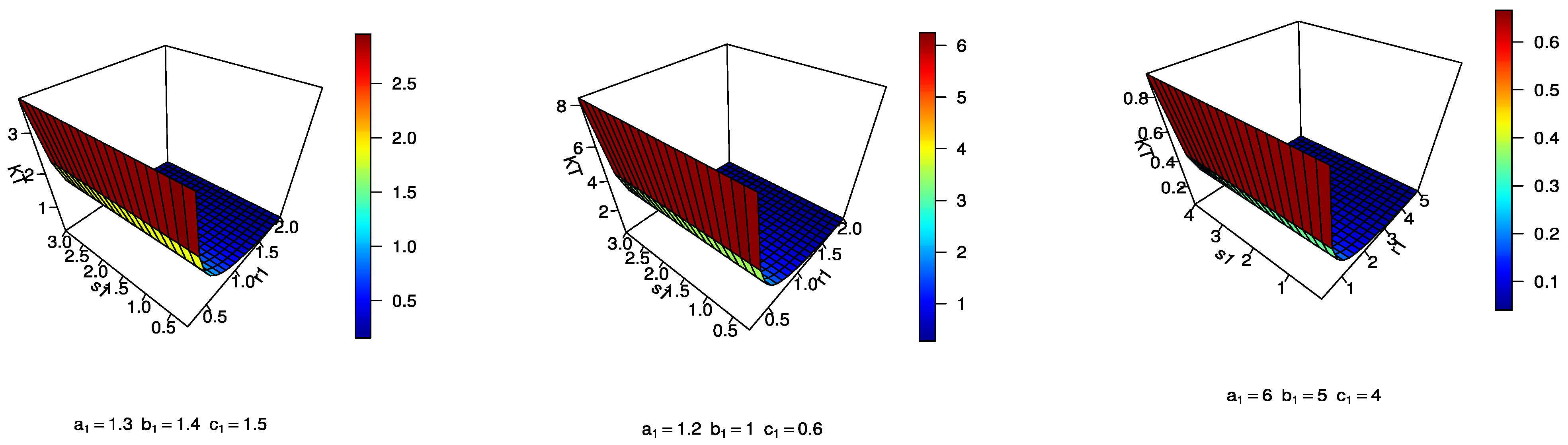
Depending on the different values of the parameters, different shapes of the pdf and the hrf of the MEKW distribution are shown in Figure 1. From Figure 1 (left panel), it appears that the MEKW pdf can include symmetric, asymmetric, right-skewed, and decreasing shapes, depending on the values of parameters. From Figure 1 (right panel), one can observe that the hrf may assume shapes with constants and that are down-upward and increasing.
The associated cdf is given by
F ( x ) = p [ 1 [ 1 [ 1 e x p ( ( x s 1 ) r 1 ) ] a 1 ] b 1 ] c 1 + q [ 1 [ 1 [ 1 e x p ( ( x s 2 ) r 2 ) ] a 2 ] b 2 ] c 2
The hazard rate function of MEKW, h r ( x ) , model is flexible, as it allows for different shapes, which is given by
h r ( x ) = f ( x ) S ( x ) = p f 1 ( x ) + q f 2 ( x ) p S 1 ( x ) + q S 2 ( x ) .
The quantile function is given by
Q j ( u ) = p G 1 { 1 [ 1 u 1 c 1 ] 1 b 1 } 1 a 1 + q G 1 { 1 [ 1 u 1 c 2 ] 1 b 2 } 1 a 2 .
In the next section, by using a quantile function-based formula for skewness and kurtosis, we plot the coefficients of skewness and kurtosis for the MEKW distribution for different values of the parameters, as shown in Figure 2. From Figure 2, one can observe that the distribution can be positively skewed, negatively skewed, and could also assume platykurtic and mesokurtic shapes.
In the next section, we discuss a strategy of estimating parameters for the EKG model under the Bayesian paradigm using independent gamma priors.

5.1. Bayesian Estimation Using Gamma Priors for the Finite Mixture of Exponentiated Kumaraswamy-G Family

In this section, we consider the Bayes estimates of the model parameters that are obtained under the assumption that the component random variables for the random vector Φ = [ a j , b j , c j , s j , r j , p , q , ] ,   f o r   j = 1 ,   2 , have independent gamma priors with hyper parameters a k   and   Ø k   ,   k = 1 , 2 , 3 , 4 , 5 , 6 , 7 , which is given by
f ( Φ ; a , Ø ) = Ø k a k Γ a k Φ a k 1 e Ø k Φ , Φ > 0 ,
By multiplying Equation (6) with the joint posterior density of the vector Φ , given the data, we can obtain the following:
π ( Φ | x _ ) L ( x | Φ ) f ( Φ ; a k , Ø k ) i = 1 m [ a 1 b 1 c 1 p g ( X i : m : n ) G a 1 1 ( X i : m : n ) [ 1 G a 1 1 ( X i : m : n ) ] b 1 1 { [ 1 G a 1 1 ( X i : m : n ) ] b 1 1 } c 1 1 [ 1 [ [ 1 G a 1 1 ( X i : m : n ) ] b 1 1 ] } c 1 ] R i + q a 2 b 2 c 2 p g ( X i : m : n ) G a 2 1 ( X i : m : n ) [ 1 G a 2 1 ( X i : m : n ) ] b 2 1 [ [ 1 G a 2 1 ( X i : m : n ) ] b 2 1 ] c 2 1 [ 1 [ [ 1 G a 2 1 ( X i : m : n ) ] b 2 1 ] c 2 ] R i ] Ø k a k Γ a k Φ a k 1 e Ø k Φ ,   I ( Φ > 0 ) .
Marginal posterior distributions of Φ can be obtained by integrating out the nuisance parameters. Next, we consider the loss function that will be used to derive the estimators from the marginal posterior distributions.

5.2. Bayes Estimation of the Vector of Parameters and Evaluation of Posterior Risk under Different Loss Functions

This section spotlights the derivation of the Bayes estimator (BE) under different loss functions and their respective posterior risks (PR). For a detailed study on different loss error functions, one can refer to [10]. The Bayes estimators are evaluated using the squared error loss function (SELF), weighted squared error loss function (WSELF), precautionary loss function (PLF), modified (quadratic) squared error loss function (M/Q SELF), logarithmic loss function (LLF), entropy loss function (ELF), and K-Loss function. The K-loss function proposed by [11] is well fitted for a measure of inaccuracy for an estimator of a scale parameter of a distribution defined by R + = ( 0 , ) ; this loss function is called the K-loss function (KLF). Table 1 shows the Bayes estimators and the associated posterior risks under each specific loss functions considered in this paper.
Next, we derive the Bayes estimators of the model parameters under different loss functions. They were originally used in estimation problems when the unbiased estimator of Φ was being considered. Another reason for its popularity is due to its relationship to the least squares theory. The SEL function makes the computations simpler. Under the SEL, WSEL, Q M S E L , PL, LL, EL and KL functions in Table 1, the Bayesian estimation for the random vector Φ = ( a j , b j , c j , s j , r j , p , q ) , for j = 1 , 2 , and under various loss functions, it can be obtained as follows.
Φ ^ S E L = E ( Φ | x _ ) = Φ ( Φ Φ ^ ) 2 π ( Φ | x _ ) d Φ .
Φ ^ W S E L = E ( Φ | x _ ) = Φ ( Φ Φ ^ ) 2 Φ π ( Φ | x _ ) d Φ .
Φ ^ Q M S E L = E ( Φ | x _ ) = Φ ( 1 Φ ^ Φ ) 2 π ( Φ | x _ ) d Φ .
Φ ^ P L = E ( Φ | x _ ) = Φ ( Φ Φ ^ ) 2 Φ ^ π ( Φ | x _ ) d Φ .
Φ ^ L L = E ( Φ | x _ ) = Φ ( l o g Φ l o g Φ ^ ) 2 π ( Φ | x _ ) d Φ .
Φ ^ K L = E ( Φ | x _ ) = Φ ( Φ ^ Φ Φ Φ ^ ) 2 π ( Φ | x _ ) d Φ .
It is evident that each of the integrals in the above section have no closed form for the resulting joint posterior distribution as given in Equation (9). Therefore, they need to be solved analytically. Consequently, the MCMC technique is proposed to generate samples from the posterior distributions and then the Bayes estimates of the parameter vector Φ are computed under progressively type II censored samples. Next, we provide the general form of the Bayesian credible intervals.

5.3. Credible Intervals

In this subsection, asymmetric 100 ( 1 τ   ) % two-sided Bayes probability interval estimates of the parameter vector Φ , denoted by [ L Φ , U Φ ] , are obtained by solving the following expression:
p [ L ( t _ ) < Φ < U ( t _ ) ] = L ( t _ ) U ( t _ ) π ( θ , β , λ | t _ ) d Φ = 1 τ .
Since it is difficult to find the interval L Φ and U Φ analytically, we apply suitable numerical techniques to solve Equation (11).

6. Bayesian Estimation of the Exponentiated Kumaraswamy Weibull Distribution

G is assumed to be the Weibull distribution with pdf and cdf, which are given by
g ( x ) = r s ( x s ) r 1 e x p [ ( x s ) r ] ,
where r is the shape parameter ( r > 0 ) , and s is the scale parameter ( s > 0 ) and
G ( x ) = ( 1 e x p [ ( x s ) r ] ) , x > 0 .  
The joint posterior density for the parameter vector Φ , given the data, becomes the following:
π ( Φ | x _ ) L ( x | Φ ) f ( Φ ; a k , Ø k ) i = 1 m [ a 1 b 1 c 1 p r 1 s 1 ( x s 1 ) r 1 1 e x p [ ( x s 1 ) r 1 ] [ 1 e x p [ ( x s 1 ) r 1 ] ] a 1 1 [ 1 [ 1 e x p [ ( x s 1 ) r 1 ] ] a 1 1 ] b 1 1 ] { [ 1 [ 1 e x p [ ( x s 1 ) r 1 ] ] a 1 1 ] b 1 1 } c 1 1 [ 1 [ [ 1 [ 1 e x p [ ( x s 1 ) r 1 ] ] a 1 1 ] b 1 1 ] c 1 ] R i + q a 2 b 2 c 2 r 2 s 2 ( x s 2 ) r 2 1 e x p [ ( x s 2 ) r 2 ] [ 1 e x p [ ( x s 2 ) r 2 ] ] a 2 1 [ 1 [ 1 e x p [ ( x s 2 ) r 2 ] ] a 2 1 ] b 2 1 [ [ 1 [ 1 e x p [ ( x s 2 ) r 2 ] ] a 2 1 ] b 2 1 ] c 2 1 [ 1 [ [ 1 [ 1 e x p [ ( x s 2 ) r 2 ] ] a 2 1 ] b 2 1 ] c 2 ] R i Ø k a k Γ a k Φ a k 1 e Ø k Φ ,   I ( Φ > 0 )
Marginal distributions of the parameter vector Φ can be obtained by integrating the nuisance parameters. Next, we consider the loss function that will be used to derive the estimators from the marginal posterior distributions.

7. Simulation Study

In this section, we evaluate the performance of the maximum likelihood and the Bayesian estimation methods to estimate the parameters using Monte Carlo simulations. We conduct the simulations using the (Maxlik) package in R software, as shown in [12]. The values of the biases, and the relative mean square errors (RMSEs) in the results indicate that the maximum likelihood and the Bayesian estimation methods performs quite well to estimate the model parameters.

Simulation Study for MEKW

In this subsection, we evaluate the performance of the maximum likelihood method and Bayesian estimation method to estimate the parameters for the MEKW model using Monte Carlo simulations. Based on progressively type II censored samples selected from the MEKW pdf in Equation (3), a total of eight parameter combinations, and assuming the sample sizes n = 25, 50, censored at 60% and 80% of the sample size, are considered. The process is repeated 1000 times and the biases (estimate–actual), RMSEs and length of confidence intervals (CI) of the estimates are reported in Table 2, Table 3, Table 4, Table 5, Table 6 and Table 7. In computing the length of CI, we obtain length asymptotic CI (LACI) for the likelihood estimators, and also obtain the length credible CI (LCCI) for the Bayesian estimators. In addition, we compared the performance of the estimation by considering the following schemes.
Scheme 1.
R k ı = 0 ,   ı = 1 , ,   n k m k
Scheme 2.
R k ı = { n k m k ,   ı = 1 0 ,   ı = 2 , , m k  
Scheme 3.
R k ı = { n k m k ,   ı = m k 0 ,   ı = 1 , , m k 1  
MLE, average bias Abs(Bias) and the RMSE for the MLE of the parameters are presented for different sample sizes and different sampling schemes
For Case 1, the selected initial values are as follows: a1 = 1.4, b1 = 1.5, c1 = 1.35, r1 = 1.7, s1 = 1.2, a2 = 1.4, b2 = 1.5, c2 = 1.35, r2 = 1.5, s2 = 1.3; p = 0.7.
For Case 2, the initial values are a1 = 1.8, b1 = 0.2, c1 = 3.5, r1 = 1.2, s1 = 1.5, a2 = 4, b2 = 0.1, c2 = 0.65, r2 = 1.5, s2 = 1.3, p = 0.6.

8. Application on Bladder Cancer Data

In this section, we provide a real data analysis to illustrate some practical applications of the proposed distributions. The data are from [13], which correspond to the remission times (in months) of a random sample of n = 128 bladder cancer patients. These data are given as follows:
0.08, 2.09, 3.48, 4.87, 6.94, 8.66, 13.11, 23.63, 0.20, 2.23, 3.52, 4.98, 6.97, 9.02, 13.29, 0.40, 2.26, 3.57, 5.06, 7.09, 9.22, 13.80, 25.74, 0.50, 2.46, 3.64, 5.09, 7.26, 9.47, 14.24, 25.82, 0.51, 2.54, 3.70, 5.17, 7.28, 9.74, 14.76, 26.31, 0.81, 2.62, 3.82, 5.32, 7.32, 10.06, 14.77, 32.15, 2.64, 3.88, 5.32, 7.39, 10.34, 14.83, 34.26, 0.90, 2.69, 4.18, 5.34, 7.59, 10.66, 15.96, 36.66, 1.05, 2.69, 4.23, 5.41, 7.62, 10.75, 16.62, 43.01, 1.19, 2.75, 4.26, 5.41, 7.63, 17.12, 46.12, 1.26, 2.83, 4.33, 5.49, 7.66, 11.25, 17.14, 79.05, 1.35, 2.87, 5.62, 7.87, 11.64, 17.36, 1.40, 3.02, 4.34, 5.71, 7.93, 11.79, 18.10, 1.46, 4.40, 5.85, 8.26, 11.98, 19.13, 1.76, 3.25, 4.50, 6.25, 8.37, 12.02, 2.02, 3.31, 4.51, 6.54, 8.53, 12.03, 20.28, 2.02, 3.36, 6.76, 12.07, 21.73, 2.07, 3.36, 6.93, 8.65, 12.63, 22.69.
Before proceeding further, we fitted the mixture EKW distribution to the complete data set. Table 8 reports the ML and Bayesian estimates for the parameters for the complete bladder cancer data. Figure 3 represents the overall fit of EKW for these data.
The validity of the fitted model is assessed by computing the Kolmogorov–Smirnov distance (KSD) statistics with p-Value KS (PVKS) in Table 8. In addition, we plotted the fitted cdf and the empirical cdf, as shown in Figure 3. This was conducted by replacing the parameters with their ML (in red) estimates, as shown in Figure 3. The KSD statistics for ML are 0.0443 and the corresponding p-value is 0.9629. Therefore, the KS test, along with Figure 3, indicate that the EKW distribution provides the best fit for this data set.
Next, we fitted the MEKW distribution to the complete data set. Table 9 reports the ML and Bayesian estimates for the parameters for the complete bladder cancer data.
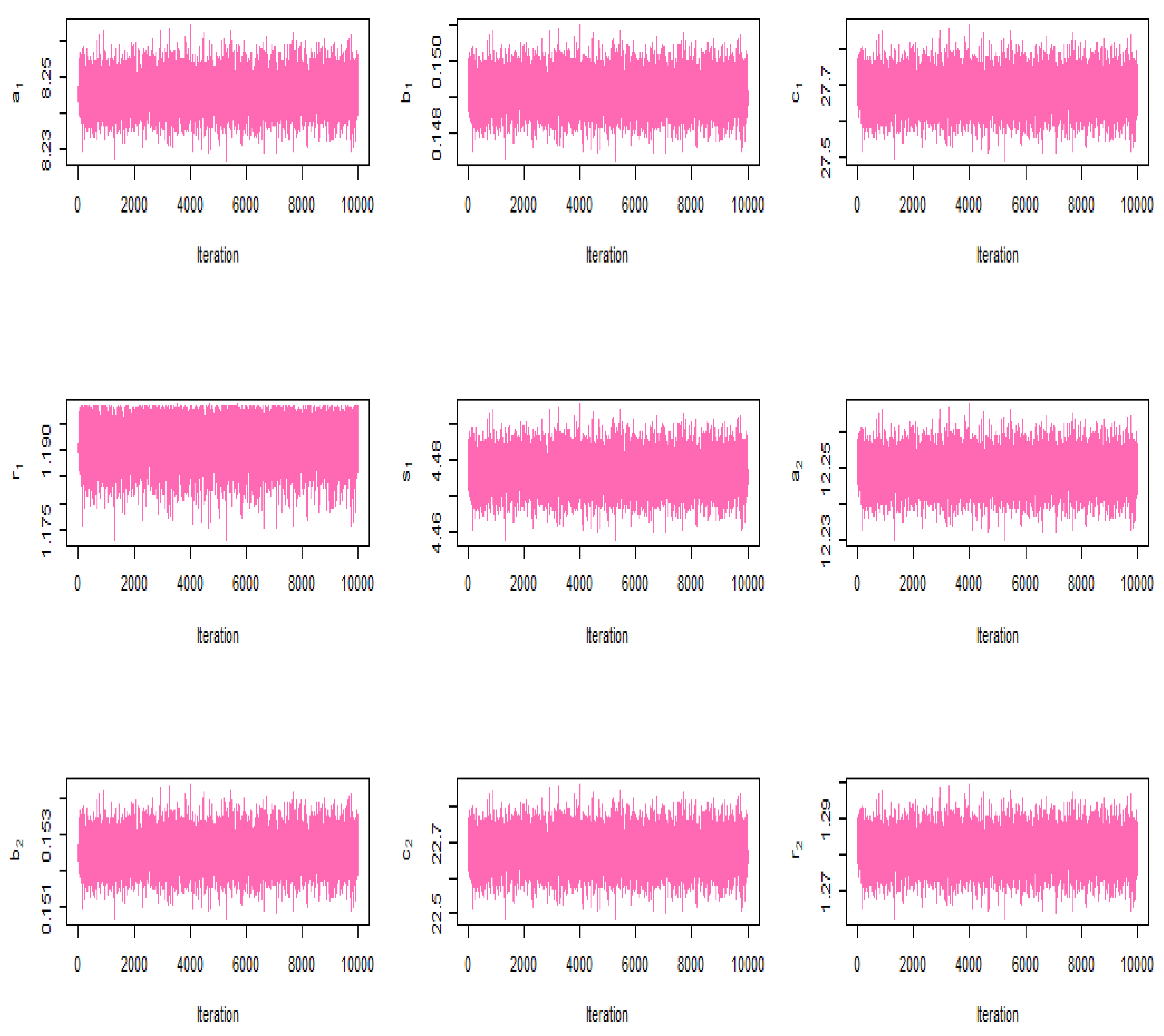
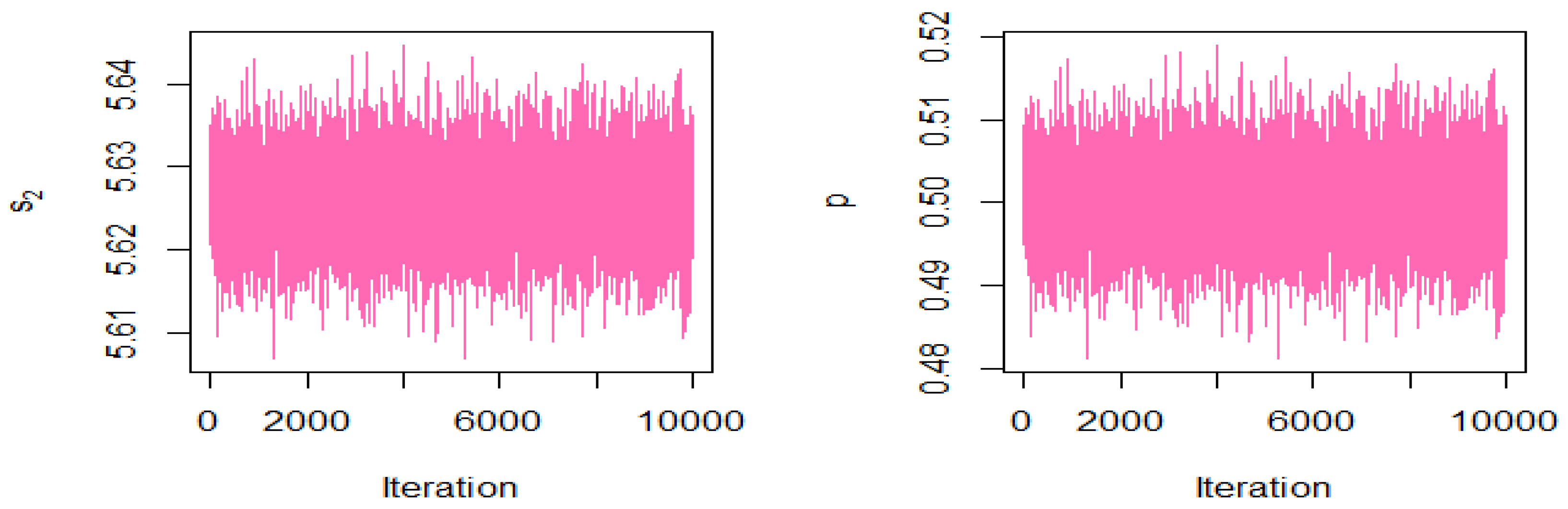
In Figure 4 and Figure 5, we provide the trace plots of the MCMC results, showing the MCMC procedure converges. Figure 6 and Figure 7 show the MCMC density and HDI intervals for the results of the Bayesian estimation of the MEKW model for the complete sample. Therefore, we will use the estimate for the mixing parameter ρ ^ = 0.5004 in computing the ML and Bayesian estimates for other parameters when using complete samples.
Two different sampling schemes are used to generate the progressively censored samples from the bladder cancer data with m = 100, which are as follows:
Strategy 1: (99*0,28); R k ı = { n k m k ,   ı = 1 0 ,   ı = 2 , , m k   (type II censoring scheme).
Strategy 2: (28,99*0); R k ı = { n k m k ,   ı = m k 0 ,   ı = 1 , , m k 1   .
In both cases, we have considered the optimization algorithm to compute the ML estimates. Table 10 shows the ML estimates for these two schemes.
For Case 1, where m = 100 and under the Scheme 1, the following can be noted: 0.08 0.20 0.40 0.50 0.51 0.81 0.90 1.05 1.19 1.26 1.35 1.40 1.46 1.76 2.02 2.02 2.07 2.09 2.23 2.26 2.46 2.54 2.62 2.64 2.69 2.69 2.75 2.83 2.87 3.02 3.25 3.31 3.36 3.36 3.48 3.52 3.57 3.64 3.70 3.82 3.88 4.18 4.23 4.26 4.33 4.34 4.40 4.50 4.51 4.87 4.98 5.06 5.09 5.17 5.32 5.32 5.34 5.41 5.41 5.49 5.62 5.71 5.85 6.25 6.54 6.76 6.93 6.94 6.97 7.09 7.26 7.28 7.32 7.39 7.59 7.62 7.63 7.66 7.87 7.93 8.26 8.37 8.53 8.65 8.66 9.02 9.22 9.47 9.74 10.06 10.34 10.66 10.75 11.25 11.64 11.79 11.98 12.02 12.03 12.07.
For Case 2, where m = 100 and under the Scheme 2, the following can be noted: 0.08 0.20 0.40 0.50 0.90 1.05 1.19 1.35 1.40 1.46 1.76 2.02 2.09 2.23 2.26 2.46 2.64 2.69 2.69 2.75 2.83 3.02 3.25 3.31 3.36 3.36 3.48 3.52 3.57 3.64 3.82 4.18 4.23 4.26 4.33 4.34 4.40 4.50 4.51 4.87 4.98 5.06 5.09 5.17 5.32 5.32 5.41 5.41 5.49 5.62 5.71 6.25 6.54 6.76 6.93 6.94 6.97 7.09 7.28 7.32 7.39 7.59 7.62 7.63 7.66 8.37 8.53 8.65 9.02 9.47 9.74 10.06 10.66 10.75 11.25 11.64 11.79 11.98 12.02 12.07 12.63 13.29 14.24 14.77 16.62 17.12 17.36 18.10 19.13 20.28 22.69 23.63 25.74 25.82 26.31 34.26 36.66 43.01 46.12 79.05.
In addition, Bayesian credible interval estimates of the parameters are obtained numerically using Markov chain Monte Carlo (MCMC) techniques. That is, samples are simulated from the joint posterior distribution in Equation (12) using the Metropolis–Hasting algorithm to obtain the posterior mean values of the estimates of the parameters by MCMC. Table 10 reports the estimates of the MEKW parameters with the corresponding SE and credible confidence intervals using the HDI algorithm of the Bayesian estimators.

9. Concluding Remarks

Finite mixture models under both the continuous and the discrete domain have received considerable attention over the last decade or so due to its flexibility of modeling an observed phenomenon when each component cannot adequately explain the entire nature of the data. In this paper, we have developed and studied a finite mixture of exponentiated Kumaraswamy-G distribution under a progressively type II censored sampling scheme, when the baseline distribution (G) is a two parameter Weibull. The efficacy of the proposed model has been established through applying it to model data from the healthcare domain. From the simulation study as well as from the application, it has been observed that, depending on the censoring scheme, either of the two estimation methods (i.e., maximum likelihood and the Bayesian estimation under independent gamma priors) could be useful. Among the various loss functions assumed for the Bayesian estimation, the results based on the small simulation study are inconclusive as to which loss function will be the most suitable for this type of finite mixture models. Most likely, a full-scale simulation study with varying parameter choices and a wide range of censoring schemes would give us an idea. Currently, we are working on this and it will be published when it is ready for submission.

Author Contributions

Conceptualization, R.A., L.A.B., E.M.A., M.K., I.G. and H.R.; Data curation, R.A.; Formal analysis, R.A., L.A.B., E.M.A., M.K. and H.R.; Funding acquisition, R.A.; Investigation, I.G.; Methodology, R.A., L.A.B., E.M.A., M.K., I.G. and H.R.; Resources, R.A.; Software, L.A.B., M.K. and H.R.; Supervision, L.A.B. and E.M.A.; Validation, L.A.B., E.M.A., I.G. and H.R.; Visualization, R.A., M.K., I.G. and H.R.; Writing—original draft, R.A., L.A.B., E.M.A., M.K., I.G. and H.R.; Writing—review & editing, I.G. All authors have read and agreed to the published version of the manuscript.

Funding

This research was funded by Princess Nourah bint Abdulrahman University Researchers Supporting Project number (PNURSP2022R50), Princess Nourah bint Abdulrahman University, Riyadh, Saudi Arabia.

Institutional Review Board Statement

Not applicable.

Informed Consent Statement

Not applicable.

Data Availability Statement

The data used to support the findings of this study are included within the article.

Acknowledgments

Princess Nourah bint Abdulrahman University Researchers Supporting Project number (PNURSP2022R50), Princess Nourah bint Abdulrahman University, Riyadh, Saudi Arabia).

Conflicts of Interest

The authors declare no conflict of interest.

Appendix A

A parameter point ε 0 in A is said to be identifiable if there is no other ε in A , which is observed to be equivalent, as shown in [14].

Appendix A.1. Necessary and Sufficient Conditions for Identifiability

(i)
Assumption 1: The structural parameters space A is an open set in m ;   = ( , + ) . This true in our case, as for Equation (3), the mixture model density. The associated parameter vector, Δ = ( a 1 , b 1 , c 1 , a 2 , b 2 , c 2 , r 1 , r 2 , s 1 , s 2 , p , q   ) , with the parameter space Ψ = { ( a 1 , a 2 ) 1 ; ( b i , c i ) ( 0 , 1 ] i = 1 , 2 ,   ( r i , s i ) + ; ( p , q ) ( 0 , 1 ] } and the associated support parameters space show that Ψ is an open set in 12 . Then, the function f is a proper density.
(ii)
Assumption 2: Functions for every Ψ . In particular, f is non-negative and the equation   f ( y ; Δ ) d y = 1 ,   holds for all Δ in Ψ . This is true for the density in Equation (3).
(iii)
Assumption 3: The sample space of y, say B, for which f is strictly positive, is the same for all Δ in the parameter space Ψ . This is also true and immeditely holds for the density in Equation (3).
(iv)
Assumption 4: For all Δ in a convex set containing Ψ and for all y in the sample space B, the functions f ( y ; Δ ) and l o g e [ f ( y ; Δ ) ] are continuously differentiable, with respect to each element in Δ . This is also true for the density in Equation (3).
(v)
Assumption 5: The elements of the information matrix (FIM) (in this case, the observed Fisher information matrix), R ( Δ ) = [ l o g f Δ i , l o g f Δ j ] , exists and are continuous functions of Δ everywhere in Ψ for the density in Equation (3); the associated log-likelihood function will be (for a single observation)
l o g [ f ( x ; Δ ) ] = l o g [ p a 1 b 1 c 1 r 1 s 1 ( x s 1 ) r 1 1 e x p [ ( x s 1 ) r 1 ] [ 1 e x p ( ( x s 1 ) r 1 ) ] a 1 1 ] [ 1 [ 1 e x p ( ( x s 1 ) r 1 ) ] a 1 ] b 1 1 [ 1 [ 1 [ 1 e x p ( ( x s 1 ) r 1 ) ] a 1 ] b 1 ] c 1 1 + q a 2 b 2 c 2 r 2 s 2 ( x s 2 ) r 2 1 e x p [ ( x s 2 ) r 2 ] [ 1 e x p ( ( x s 2 ) r 2 ) ] a 2 1 [ 1 [ 1 e x p ( ( x s 2 ) r 2 ) ] a 2 ] b 2 1 [ 1 [ 1 [ 1 e x p ( ( x s 2 ) r 2 ) ] a 2 ] b 2 ] c 2 1 ]
For illustrative purposes, we will discuss one element from the observed FIM of dimension 12 × 12. The proof of existence of the remaining elements and continuity can be similarly established. For brevity, the complete details are avoided. It is available upon request to the authors. Next, one must consider
2 l o g f a 1 a 2 = D 1 D 2
where
D 1 = [ b 1 b 2 c 1 c 2 e x p [ ( x s 1 ) r 1 + ( x s 2 ) r 2 ] [ 1 e x p ( ( x s 1 ) r 1 ) ] a 1 [ 1 e x p ( ( x s 2 ) r 2 ) ] a 2 [ 1 [ 1 e x p ( ( x s 1 ) r 1 ) ] a 1 ] b 1 2 [ 1 [ 1 e x p ( ( x s 2 ) r 2 ) ] a 2 ] b 2 2 [ 1 [ 1 [ 1 e x p ( ( x s 1 ) r 1 ) ] a 1 ] b 1 ] c 1 1 [ 1 [ 1 [ 1 e x p ( ( x s 2 ) r 2 ) ] a 2 ] b 2 ] c 2 2 p q r 1 r 2 ( x s 1 ) r 1 ( x s 2 ) r 2 ( 1 + [ 1 e x p ( ( x s 1 ) r 1 ) ] a 1 ) ( 1 + [ 1 [ 1 e x p ( ( x s 1 ) r 1 ) ] a 1 ] b 1 ) + a 1 ( 1 [ 1 [ 1 e x p ( ( x s 1 ) r 1 ) ] a 1 ] b 1 ) + b 1 [ 1 e x p ( ( x s 1 ) r 1 ) ] a 1 ( 1 + c 1 [ 1 [ 1 e x p ( ( x s 1 ) r 1 ) ] a 1 ] b 1 ) l o g [ 1 e x p ( ( x s 1 ) r 1 ) ] ( 1 + [ 1 e x p ( ( x s 2 ) r 2 ) ] a 2 ) ( 1 + [ 1 [ 1 e x p ( ( x s 2 ) r 2 ) ] a 2 ] b 2 ) a 2 b 2 ( 1 [ 1 [ 1 e x p ( ( x s 2 ) r 2 ) ] a 2 ] b 2 ) + l o g [ 1 e x p ( ( x s 2 ) r 2 ) ] ( 1 + c 2 [ 1 [ 1 e x p ( ( x s 2 ) r 2 ) ] a 2 ] b 2 ) ] ,
D 2 = ( 1 + e x p ( ( x s 1 ) r 1 ) ) ( 1 + e x p ( ( x s 2 ) r 2 ) ) [ p r 1 a 1 b 1 c 1 [ 1 e x p ( ( x s 1 ) r 1 ) ] a 1 1 [ 1 [ 1 e x p ( ( x s 1 ) r 1 ) ] a 1 ] b 1 1 [ 1 [ 1 [ 1 e x p ( ( x s 1 ) r 1 ) ] a 1 ] b 1 ] c 1 1 ( x s 1 ) r 1 + q r 2 a 2 b 2 c 2 [ 1 e x p ( ( x s 2 ) r 2 ) ] a 2 1 [ 1 [ 1 e x p ( ( x s 2 ) r 2 ) ] a 2 ] b 2 1 [ 1 [ 1 [ 1 e x p ( ( x s 2 ) r 2 ) ] a 2 ] b 2 ] c 2 1 ( x s 2 ) r 2 ] 2
From Equation (A1), it is obvious that these derivatives exist for all possible choices of the parameter vector Δ and for the parameter space Ψ , as well as for all possible values of x ( 0 , ) . This derivative function is also continuous. The proof is simple, and thus excluded.
  • Identifiability of the MEKW Model
Before considering the aspect of estimation and associated inference and classification of random variables, which are based on observations from a mixture, it is necessary to address the subject of identifiability of the mixture(s) and possibly its components. We suggest our readers to refer to the following pertinent reference: [14] for more information on the identifiability of mixture distributions. The identification of a mixture for two EK (with the same baseline G’s as given in (2)) components will now be explored.
We begin with the combination of two survival functions. One must consider a linear combination of two separate distributions, one of which is EKW ( a 1 , b 1 , c 1 , s 1 , r 1 ) distribution, and the other distribution is EKW ( a 2 , b 2 , c 2 , s 2 , r 2 ) , as shown below.
i = 0 2 p i S i ( x ) = 0 ,
where S 1 ( x ) = 1 [ 1 [ 1 [ 1 e x p ( ( x s 1 ) r 1 ) ] a 1 ] b 1 ] c 1 ,   0 < x < ,   a 1 , b 1 , c 1 , s 1 , r 1 > 0 , S 2 ( x ) = 1 { 1 [ 1 ( 1 e x p [ ( x s 2 ) r 2 ] ) a 2 ] b 2 } c 2 ,   0 < x < ,   a 2 , b 2 , c 2 , s 2 , r 2 > 0 , and p 1 and p 2 are the mixing weights, such that p 1 + p 2 = 1 and 0 < p i < 1     i = 1 , 2 . The finite mixture of EKW ( a 1 , b 1 , c 1 , s 1 , r 1 ) , and EKW ( a 2 , b 2 , c 2 , s 2 , r 2 ) distributions are identifiable, if S 1 ( x ) ,   S 2 ( x ) are linearly independent. This means, if ( a 1 , b 1 , c 1 , s 1 , r 1 ) ( a 2 , b 2 , c 2 , s 2 , r 2 ) , this implies p 1 = p 2 = 0 .
If x = 0 , then S 1 ( 0 ) = S 2 ( 0 ) = 1   p 1 + p 2 = 0 p 1 = p 2 .
Then,
1 [ 1 [ 1 [ 1 e x p ( ( x s 1 ) r 1 ) ] a 1 ] b 1 ] c 1 = 1 { 1 [ 1 ( 1 e x p [ ( x s 2 ) r 2 ] ) a 2 ] b 2 } c 2 ,
[ 1 [ 1 [ 1 e x p ( ( x s 1 ) r 1 ) ] a 1 ] b 1 ] c 1 = { 1 [ 1 ( 1 e x p [ ( x s 2 ) r 2 ] ) a 2 ] b 2 } c 2 ,
i 1 = 0 ( c 1 i 1 ) ( 1 ) i 1 ( 1 ( 1 e x p ( ( x s 1 ) r 1 ) ) a 1 ) b 1 i 1 = i 2 = 0 ( c 2 i 1 ) ( 1 ) i 1 ( 1 ( 1 e x p ( ( x s 2 ) r 2 ) ) a 2 ) b 2 i 1 ,
i 1 = 0 ( c 1 i 1 ) i 2 = 0 ( b 1 i 1 i 2 ) ( 1 ) i 1 + i 2 ( 1 e x p ( ( x s 1 ) r 1 ) ) a 1 i 2 = i 1 = 0 ( c 2 i 1 ) i 2 = 0 ( b 2 i 1 i 2 ) ( 1 ) i 1 + i 2 [ e x p ( ( x s 2 ) r 2 ) ] a 2 i 2 ,
i 1 = 0 ( c 1 i 1 ) i 2 = 0 ( b 1 i 1 i 2 ) ( 1 ) i 1 + i 2 i 3 = 0 ( a 1 i 2 i 3 ) ( 1 ) i 1 + i 2 + i 3 ( e x p ( ( x s 1 ) r 1 ) ) = i 1 = 0 ( c 2 i 1 ) i 2 = 0 ( b 2 i 1 i 2 ) ( 1 ) i 1 + i 2 i 3 = 0 ( a 2 i 2 i 3 ) ( 1 ) i 1 + i 2 + i 3 ( e x p ( ( x s 2 ) r 2 ) ) ,
i 1 = 0 ( c 1 i 1 ) i 2 = 0 ( b 1 i 1 i 2 ) ( 1 ) i 1 + i 2 i 3 = 0 ( a 1 i 2 i 3 ) ( 1 ) i 1 + i 2 + i 3 ( x s 1 ) r 1 = i 1 = 0 ( c 2 i 1 ) i 2 = 0 ( b 2 i 1 i 2 ) ( 1 ) i 1 + i 2 i 3 = 0 ( a 2 i 2 i 3 ) ( 1 ) i 1 + i 2 + i 3 ( x s 2 ) r 2
where i 1 ! = i 1 ( i 1 1 ) ( i 1 2 ) .3.2.1 , i 1 = i 2 = i 3 , and the coefficients of x on both sides are compared and it is discovered that a 1 = a 2 ,   b 1 = b 2 ,   c 1 = c 2 ,   s 1 = s 2   ,   r 1 = r 2 ,   and p 1 = p 2 = 0 .
S 1 ( x ) and S 2 ( x ) are, thus, linearly independent. As a result, the EKW ( a 1 , b 1 , c 1 , s 1 , r 1 ) and EKW ( a 2 , b 2 , c 2 , s 2 , r 2 ) distributions can be identified as a finite mixture.

References

  1. Al Alotaibi, R.; Almetwally, E.M.; Ghosh, I.; Rezk, H. Classical and Bayesian inference on finite mixture of exponentiated Kumaraswamy Gompertz and exponentiated Kumaraswamy Frechet distributions under progressive Type II censoring with applications. Mathematics 2022, 10, 1496. [Google Scholar] [CrossRef]
  2. Tahir, M.H.; Nadarajah, S. Parameter induction in continuous univariate distributions: Well-established G families. Ann. Braz. Acad. Sci. 2015, 87, 539–568. [Google Scholar] [CrossRef] [PubMed]
  3. Lemonte, J.A.; Barreto-Souza, W.; Cordeiro, M.G. The exponentiated Kumaraswamy distribution and its log-transform. Braz. J. Probab. Stat. 2003, 27, 31–53. [Google Scholar] [CrossRef]
  4. Alzaghal, A.; Felix, F.; Carl, L. Exponentiated T-X family of distributions with some applications. Int. J. Stat. Probab. 2013, 2, 31–49. [Google Scholar] [CrossRef] [Green Version]
  5. Nadarajah, S.; Rocha, R. Newdistns: An R Package for new families of distributions. J. Stat. Softw. 2016, 69, 1–32. [Google Scholar] [CrossRef] [Green Version]
  6. Mudholkar, G.S.; Srivastava, D.K.; Kollia, G.D. A generalization of the Weibull distribution with application to the analysis of survival data. J. Am. Stat. Assoc. 1996, 91, 1575–1583. [Google Scholar] [CrossRef]
  7. Gupta, R.C.; Gupta, P.L.; Gupta, R.D. Modeling failure time data by Lehman alternatives. Comm. Statist. Theory Methods 1998, 27, 887–904. [Google Scholar] [CrossRef]
  8. Nadarajah, S.; Bakouch, H.S.; Tahmabi, R. Ageneralized Lindley distribution. Sankhya B 2011, 73, 331–359. [Google Scholar] [CrossRef]
  9. Blanchet, J.H.; Sigman, K. On exact sampling of stochastic perpetuilies. J. Appl. Probab. 2011, 48A, 165–182. [Google Scholar] [CrossRef] [Green Version]
  10. Ali, S.; Aslam, M.; Mohsin, S.; Kazmi, A. A study of the effect of the loss function on Bayes estimate, posterior risk and hazard function for Lindley distribution. Appl. Math. Model. 2013, 23, 6068–6078. [Google Scholar] [CrossRef]
  11. Wasan, M.T. Parametric Estimation; Mcgraw-Hill: New York, NY, USA, 1970. [Google Scholar]
  12. R Core Team. R: A Language and Environment for Statistical Computing; R Foundation for Statistical Computing: Vienna, Austria, 2019; Available online: https://www.R-project.org/ (accessed on 12 July 2022).
  13. Lee, E.T.; Wang, J. Statistical Methods for Survival Data Analysis; John Wiley & Sons: New York, NY, USA, 2003; 476p. [Google Scholar]
  14. Rothenberg, T.J. Identification in Parametric Models. Econometrica 1971, 39, 577–591. [Google Scholar] [CrossRef]
Figure 1. The pdf and hrf of the MEKW model for different values of its parameters.
Mathematics 10 02800 g001
Figure 2. Coefficients of skewness and kurtosis for EKW distribution.
Mathematics 10 02800 g002aMathematics 10 02800 g002b
Figure 3. ML estimates of the EKW parameters for the complete bladder cancer data.
Mathematics 10 02800 g003
Figure 4. MCMC trace for results of Bayesian estimation of model for complete Bladder data for first 9 parameters.
Mathematics 10 02800 g004
Figure 5. MCMC trace for results of Bayesian estimation of model for complete Bladder data for the last two parameters.
Mathematics 10 02800 g005
Figure 6. MCMC density and HDI intervals for results of Bayesian estimation of model for complete Bladder data for 9 parameters.
Mathematics 10 02800 g006
Figure 7. MCMC density and HDI intervals for the Bayesian estimation of model for complete Bladder data for the last two parameters.
Mathematics 10 02800 g007
Table 1. Bayes estimator and posterior risk under different loss functions.
Loss FunctionBayes Estimator (BE)Posterior Risk (PR)
L 1 = S E L = ( Φ Φ ^ ) 2 E ( Φ | X ) V ( Φ | X )
L 2 = W S E L = ( Φ Φ ^ ) 2 Φ [ E ( Φ 1 | X ) ] 1 E ( Φ | X ) [ E ( Φ 1 | X ) ] 1
L 3 = Q M S E L = ( 1 Φ ^ Φ ) 2 E ( Φ 1 | X ) E ( Φ 2 | X ) 1 E ( Φ 1 | X ) 2 E ( Φ 2 | X )
L 4 = P L = ( Φ Φ ^ ) 2 Φ ^ E ( Φ 2 | X ) 2 [ E ( Φ 2 | X ) E ( Φ | X ) ]
L 5 = L L = ( l o g Φ l o g Φ ^ ) 2 e x p [ E ( l o g Φ | X ) ] V ( l o g Φ | X )
L 6 = E L = ( Φ ^ Φ l o g Φ Φ ^ 1 ) [ E ( Φ 1 | X ) ] 1 E ( l o g Φ | X ) l o g E ( Φ 1 | X )
L 7 = K L = ( Φ ^ Φ Φ Φ ^ ) 2 E ( Φ | X ) E ( Φ 1 | X ) 2 [ E ( Φ | X ) E ( Φ 1 | X ) 1 ]
Table 2. Bias, RMSE and length of CI for the MLE and Bayesian estimates of the parameters are presented for different sample sizes: Scheme 1 (complete sample), Case 1.
MLEBayesian
n BiasRMSELACIBiasRMSELCCI
25a10.13630.74672.88090.07430.25690.9628
b1−0.21610.77582.92360.10910.22750.7848
c10.13740.94823.68140.09410.29200.9927
r10.68831.25194.10300.14410.27830.8962
s1−0.10830.38191.43690.02430.14260.5350
a20.21190.88363.36590.10800.24990.8166
b2−0.29850.84083.08420.14320.31191.0558
c20.29081.03643.90340.03800.22240.8259
r20.77341.40024.58010.14380.28550.9685
s2−0.20230.50341.80880.00520.03350.1289
p−0.01120.09520.3710−0.03420.08850.3028
50a10.03250.62532.45020.03640.16480.6325
b1−0.18650.64402.41850.06020.13330.4764
c10.00060.74572.92590.02620.16340.6277
r10.58670.99233.14010.11020.18350.5522
s1−0.03600.30251.17840.01030.08980.3480
a20.10640.75232.92250.03640.13890.5130
b2−0.19270.66042.47840.11010.22160.7209
c20.15010.89133.44750.03960.14700.5468
r20.60111.06773.46250.09780.17560.5552
s2−0.10980.41711.57900.00000.02190.0854
p−0.00120.06480.2540−0.01460.06220.2353
100a1−0.07760.50131.94340.01560.12050.4462
b1−0.16080.54002.02280.05060.11930.4208
c1−0.14540.57452.18090.01360.14120.5552
r10.63210.91612.60220.10300.16090.4740
s10.03690.26111.0143−0.00100.07010.2702
a20.05650.64702.52890.01620.10040.3790
b2−0.12450.60242.31280.06730.15830.5709
c20.00530.77043.02300.02030.11380.4199
r20.50950.91322.97410.07130.13960.4697
s2−0.02140.36871.4443−0.00050.01790.0671
p0.00190.05210.2043−0.00500.04970.1896
Table 3. Bias, RMSE and length of CI for the MLE and Bayesian estimates of the parameters are presented for different schemes: Case 1 and n = 25.
MLEBayesian
Schemen, m BiasRMSELACIBiasRMSELCCI
225, 15a10.20860.69352.59500.11570.27750.9395
b1−0.35160.78582.75760.09110.22820.7983
c10.15110.75692.91010.07650.26760.9211
r10.59211.18014.00560.14780.35111.1950
s1−0.24180.43281.40850.03660.22400.8323
a20.34630.94753.46050.02170.22950.8224
b2−0.41460.93813.30210.21700.42211.4613
c20.25050.89013.35150.04710.25190.9327
r21.11891.57924.37270.14650.29420.9666
s2−0.45160.64201.7906−0.00910.04360.1606
p0.02320.21150.8248−0.00540.18030.5545
25, 20a10.17070.68972.56220.04550.14390.5135
b1−0.34380.77052.70600.05000.13410.4665
c10.03160.74942.90380.04360.15660.5762
r10.65381.03143.34740.05710.20670.7663
s1−0.17990.40671.31440.04040.14910.5154
a20.27470.87313.25210.03710.15070.5460
b2−0.31550.80022.88540.10400.25570.8661
c20.20940.80933.05560.03540.14280.5314
r20.96091.26343.01200.09990.19880.6814
s2−0.29520.51441.6531−0.00300.02500.0908
p0.00990.13390.5238−0.01690.11430.4068
325, 15a10.11610.71572.77130.09090.25820.9175
b1−0.39360.78692.67370.09940.22080.7204
c10.16170.85773.30510.06830.26320.9451
r10.62091.28264.40380.10230.28850.9627
s1−0.17450.43391.55870.07540.17320.6193
a20.29770.89053.29330.08590.23250.8070
b2−0.34940.81022.86820.11310.31681.0870
c20.35930.95703.48060.09300.25290.8532
r20.74861.28814.11320.13100.28760.9885
s2−0.25230.50781.72930.00910.03470.1240
p−0.01100.21580.8458−0.03550.18840.5606
25, 20a10.16070.71282.72500.05630.14890.5512
b1−0.21650.70842.51940.05020.12470.4392
c10.12490.81003.07880.04700.16340.6065
r10.59431.03223.63340.06500.19160.6970
s1−0.15540.40231.45620.02350.10690.4019
a20.18880.86843.26220.05520.13650.4698
b2−0.29370.81152.69680.06140.19840.6992
c20.29930.80633.00350.04730.14000.5285
r20.58071.04574.07570.07320.18290.6418
s2−0.16630.50841.48850.00480.02000.0761
p−0.01070.14190.5554−0.03540.12670.4211
Table 4. Bias, RMSE and length of CI for the MLE and Bayesian estimates of the parameters are presented for different schemes: Case 1 and n = 50.
MLEBayesian
Schemen, m BiasRMSELACIBiasRMSELCCI
250, 30a10.17400.64642.44280.09850.26860.9424
b1−0.28390.68502.44610.10490.26270.9051
c10.05350.66842.61430.08150.28620.9613
r10.45361.03293.64130.13230.37221.2898
s1−0.17680.39141.37010.04620.23670.8292
a20.15380.78033.0018−0.00470.24900.9586
b2−0.31400.74852.66610.32060.54881.6380
c20.06640.75852.96490.02450.25440.9684
r21.12361.61304.54120.21030.36691.1379
s2−0.35360.54991.6526−0.02640.06370.2052
p0.02730.19370.75270.01090.17740.5251
50, 40a10.13850.60582.35260.03780.15150.5607
b1−0.32160.68632.37920.03570.14020.5168
c10.04960.58072.51460.03180.17570.6541
r10.45280.91193.59980.06710.22310.7929
s1−0.14350.37821.37320.04880.15140.5324
a20.16690.77592.97310.01340.15140.5693
b2−0.17640.74962.58590.17890.33020.9973
c2−0.01990.73982.90200.01290.14120.5300
r21.04211.55714.53990.14200.25640.8151
s2−0.20030.42521.4718−0.01210.03420.1166
p0.02610.11700.44750.00950.10470.3537
350, 30a10.10310.64982.51740.07790.26540.9538
b1−0.21740.66652.47240.09680.24330.8425
c10.15990.78873.03060.08040.30271.0356
r10.38910.99083.57570.08070.25520.9065
s1−0.11310.37221.39150.05460.15870.5932
a20.20470.71342.68170.09210.23520.7769
b2−0.18240.69742.64140.08140.28370.9804
c20.20890.85283.24430.05720.23730.8509
r20.40220.91463.22310.11080.27150.9205
s2−0.14850.43581.60760.01240.03680.1380
p−0.00580.20600.8079−0.01900.19040.5459
50, 40a10.19190.60642.49340.04570.14690.5373
b1−0.13600.62662.40020.05010.13530.4797
c10.20240.63062.92150.03710.16460.6183
r10.25770.87363.27530.04440.17670.6505
s1−0.11010.36091.34850.03330.09970.3671
a20.18380.70482.58440.03890.13820.5167
b2−0.18980.69132.60810.05030.18260.6657
c20.22090.84923.15140.03550.14050.5139
r20.48170.90323.15830.06660.17640.6511
s2−0.13630.40601.57240.00400.02330.0878
p−0.01060.11940.4667−0.02380.11200.3631
Table 5. Bias, RMSE and length of CI for the MLE and Bayesian estimates of the parameters are presented for different sample sizes: Scheme 1 (complete sample), Case 2.
MLEBayesian
n BiasRMSELACIBiasRMSELCCI
25a10.49501.25855.90780.10460.27250.9632
b10.00250.09740.38190.06910.08110.3175
c10.33921.25564.74360.06630.17570.6258
r10.11660.24920.8640−0.01890.14580.5568
s10.13380.45681.71380.18190.28230.8286
a20.08501.90857.48140.03980.10790.3711
b20.04610.12450.45400.03120.06750.2063
c20.25990.56431.96560.04750.23130.7513
r20.09840.34441.2950−0.05340.19930.7545
s2−0.00480.36951.44970.02160.03820.1283
p−0.00350.09200.3607−0.01160.08160.3071
50a10.25321.07814.91560.06150.17270.6082
b10.00390.07740.30320.04250.07780.2230
c10.32671.09004.08060.03390.11890.4407
r10.07740.15880.5440−0.01280.10090.3987
s10.10670.43141.64010.09850.17550.5609
a2−0.16251.48095.77590.02990.07810.2910
b20.04570.11830.42810.02960.05150.1509
c20.24150.46341.82990.04100.16410.5968
r20.03690.23090.8944−0.06550.13060.4482
s20.03140.30731.45690.01570.02650.0823
p−0.00360.06920.2712−0.00940.06480.2451
100a10.10000.95193.71450.03970.15580.5863
b10.00540.05220.20370.02490.05390.1661
c10.28330.79832.92860.03490.11580.4385
r10.05340.11290.39030.00630.07760.3142
s10.06880.31421.20300.06580.14100.4920
a2−0.17311.15504.48110.01990.07320.2684
b20.03960.09850.35410.02330.03810.1088
c20.13590.30421.06770.01740.10190.3844
r20.00060.13040.5117−0.05660.09780.3237
s20.03630.23201.24650.01140.02540.0740
p−0.00140.04850.1903−0.00310.04720.1834
Table 6. Bias, RMSE and length of CI for the MLE and Bayesian estimates of the parameters are presented for different schemes: Case 2 and n = 25.
MLEBayesian
Schemen, m BiasRMSELACIBiasRMSELCCI
225, 15a10.32191.50065.75110.08900.26090.9529
b1−0.01400.10610.41250.04090.10460.3430
c10.24751.30185.01490.03030.16800.6187
r10.30450.60542.05330.10030.25110.8449
s10.17600.58712.19800.14230.25440.7830
a2−0.10572.03647.98000.03730.10590.3868
b20.05330.21030.79820.02600.06790.2227
c20.25140.61902.21980.04910.21890.7067
r20.24210.58002.0680−0.00260.23040.9165
s20.12300.57062.18650.02030.03620.1182
p−0.02300.15440.5992−0.03200.13710.5096
25, 20a10.44501.27724.72920.05020.14320.5073
b1−0.00710.10400.40720.03910.09900.3048
c10.27641.20674.60920.02350.10100.3778
r10.19540.40301.38300.03090.17680.6555
s10.14610.50491.89650.08190.15890.5218
a20.19442.04507.98800.02350.06270.2217
b20.03410.13790.52420.02390.05810.1891
c20.22560.60542.20440.05510.20440.7016
r20.15820.40931.4811−0.05060.17080.6461
s20.07120.43721.69250.01270.02230.0712
p−0.02000.11780.4557−0.03140.10560.3854
325, 15a10.37561.54665.88710.09770.24910.8675
b10.00860.11490.44970.07280.10160.3220
c10.24021.16524.47400.04070.15760.6094
r10.15130.28970.9695−0.02670.14920.5809
s10.21960.56392.03820.15170.26450.8215
a20.02201.82207.14900.04730.11380.3973
b20.04560.15890.59710.02890.06580.2128
c20.26860.60842.14200.09570.25100.8332
r20.24900.47891.6053−0.01770.21340.8030
s20.10150.46971.79950.02460.04060.1244
p−0.17500.20050.3840−0.15990.18140.3204
25, 20a10.33451.43885.49090.05560.15090.5303
b10.00260.10350.40580.05040.09420.2754
c10.35661.02764.28070.02910.10150.3685
r10.14130.26190.8653−0.01600.12500.4882
s10.18980.55212.03460.09600.16260.5275
a20.20651.78825.33900.02420.06220.2171
b20.05230.14220.51900.02180.05660.1773
c20.32280.54612.02350.06670.20280.7112
r20.15090.41651.5231−0.03440.15650.5786
s20.05760.41801.62470.01280.02320.0730
p−0.08590.12940.3797−0.07730.11710.3043
Table 7. Bias, RMSE and length of CI for the MLE and Bayesian estimates of the parameters are presented for different schemes: Case 2 and n = 50.
MLEBayesian
Schemen, m BiasRMSELACIBiasRMSELCCI
I50, 30a10.16071.16244.51750.09500.27560.9877
b1−0.01560.09260.35830.04250.11560.3975
c10.14100.95503.70640.03400.18040.7061
r10.35820.69972.35860.13900.31041.0253
s10.16870.61282.31150.13470.27300.8936
a2−0.39251.42245.36480.04660.11480.4057
b20.04440.15380.57790.02330.06430.2126
c20.17070.40401.43680.06210.21320.7099
r20.26140.65992.37760.03530.25890.9918
s20.18040.67392.54790.01920.03940.1334
p−0.04400.20160.7719−0.04790.18590.5668
50, 40a10.13221.03654.20450.06160.18230.6517
b1−0.00610.09030.35360.02180.08000.2685
c10.14060.90283.69850.02140.11050.4222
r10.16190.36061.26420.06060.18100.6664
s10.12290.43181.62430.06730.15320.5163
a2−0.20441.35524.50380.02190.06980.2580
b20.02860.11660.44350.02240.04980.1704
c20.16820.37411.40340.05000.17030.5965
r20.12310.34051.2457−0.02940.15680.6370
s20.06470.48491.88590.01070.02380.0771
p−0.01170.10500.4094−0.01710.09960.3911
II50, 30a10.34281.24794.70830.11730.30371.1006
b10.00190.08560.33570.06510.10780.2946
c10.26101.05484.01040.06310.18390.6537
r10.12520.22710.7435−0.01330.12840.5061
s10.16250.40281.44610.17080.28070.7910
a2−0.01891.23754.85530.05950.12380.4057
b20.03000.09860.36840.03440.06260.1887
c20.16870.37441.31150.11120.23000.7343
r20.13280.30411.0733−0.06240.16940.5980
s20.08930.34741.31740.03020.04800.1460
p−0.24140.25010.2563−0.22610.23450.2025
50, 40a10.13230.95044.62440.06020.17190.6060
b10.00840.08550.33370.04880.08860.2672
c10.27950.81443.83520.03550.11760.4267
r10.09500.18490.6223−0.01750.10770.4235
s10.15390.39121.41140.09580.17420.5624
a2−0.15100.94354.59930.02800.07480.2571
b20.04060.09140.34400.02390.04830.1573
c20.12760.34281.25320.05240.16990.6015
r20.10080.29561.0090−0.04750.13780.4887
s20.08800.30421.24620.01330.02580.0864
p−0.12120.13660.2472−0.11480.12980.1923
Table 8. ML estimates of the EKW parameters with the corresponding bladder data.
abcrsKSDPVKSCVMAD
Estimates3.65373.11791.13110.45785.28730.04430.96290.04080.2700
Table 9. ML estimates of the MEKW parameters for the complete sample of the bladder data.
MLEBayesian
EstimatesSELowerUpperEstimatesSELowerUpper
a18.24590.01718.21258.27948.32970.00758.23108.2601
b10.14910.01230.12500.17330.18660.00080.14770.1506
c127.68257.531412.920842.444127.25780.197527.532727.8240
r11.19250.00151.18961.19541.14560.00151.18001.1984
s14.47700.00144.47424.47984.30290.00034.46204.4911
a212.24920.007912.233712.264812.22000.007512.234312.2634
b20.15260.01260.12790.17730.22070.00080.15110.1540
c222.67635.806311.296034.056722.67200.075422.526622.8179
r21.28100.00241.27631.28580.30400.00141.26611.2952
s25.62610.00265.62105.63130.19220.00255.61155.6406
p0.50040.03470.43250.56840.60390.00750.48580.5149
Table 10. ML estimates of the MEKW parameters for different censoring schemes of the bladder data.
MLEBayesian
m EstimatesSEEstimatesSELowerUpper
100I10.77980.66662.33790.14432.08312.5781
20.37010.29451.40050.11411.10891.5987
31.58901.56421.02170.09290.87471.2007
41.04760.31450.67160.06070.56070.8075
52.59981.46556.16280.13885.93276.4243
60.35850.40150.40150.06890.25640.5199
70.09100.15590.33540.05650.25260.4543
82.27881.92974.15020.12573.92164.3922
90.88010.26300.65980.04610.57200.7408
100.32630.41070.70230.10300.48120.8705
110.49960.03120.49780.03070.43200.5622
II13.10951.21152.98650.85781.38654.5300
25.43661.21155.57200.59854.74507.8209
31.61541.57052.07210.98250.42633.9153
40.38950.54880.39890.08170.24330.5639
59.47013.054610.12712.19455.807714.0496
63.13910.20303.22030.15362.17663.9201
75.38164.73746.04172.59531.847711.4996
81.60351.57621.85111.12090.44484.2545
90.38910.35440.41270.14050.19920.7092
109.22415.637611.13514.86383.141819.6341
110.50000.03120.50310.02450.41460.5892
Publisher’s Note: MDPI stays neutral with regard to jurisdictional claims in published maps and institutional affiliations.

