A Novel Divisional Bisection Method for the Symmetric Tridiagonal Eigenvalue Problem

Abstract

The embarrassingly parallel nature of the Bisection Algorithm makes it easy and efficient to program on a parallel computer, but with an expensive time cost when all symmetric tridiagonal eigenvalues are wanted. In addition, few methods can calculate a single eigenvalue in parallel for now, especially in a specific order. This paper solves the issue with a new approach that can parallelize the Bisection iteration. Some pseudocodes and numerical results are presented. It shows our algorithm reduces the time cost by more than 35–70% compared to the Bisection algorithm while maintaining its accuracy and flexibility.

1. Introduction

The symmetric tridiagonal matrices often arise as primary data in many computational quantum physical [1,2], mathematical [3,4,5], dynamical [6,7], computational quantum chemical [8,9], signal processing [10], or even medical [11] problems and hence are important. The current software reduces the generalized and the standard symmetric eigenproblems to a symmetric tridiagonal eigenproblem as a common practice [10,12,13]. What is more interesting is that the opposite path is also productive. Marques [14] computes the SVD of a bidiagonal matrix through the eigenpairs of an associated symmetric tridiagonal matrix. In this paper, we focus on symmetric eigenvalue solving.

People desire a parallel algorithm of good performance and flexibility, especially today as CPU cores and massively parallel technology have skyrocketed. We noticed that in many application scenes of eigenvalue computation, for example, in dynamics, it is often necessary to solve only the first few orders of eigenvalues of a large matrix. The desire for the largest eigenvalue is also common in practice [15,16,17]. However, the current QR, MRRR (Multiple Relatively Robust Representations), DC (Divided and Conquer), and Bisection algorithms do not seem to perform sufficient parallel operations if the number of CPU cores (say, 40) is significantly larger than the number of eigenvalues (say, 1) to be solved.

The most popular algorithm at present for a symmetric eigenproblem is the QR algorithm because of its stability and computational efficiency [18,19,20]. When only eigenvalues are desired, all square roots can be eliminated in the QR transformation. This was first observed by Ortega and Kaiser in 1963 [21] and a fast, stable algorithm was developed by Pal, Walker, and Kahan (PWK) in 1969 [22]. However, the parallelization of the QR algorithm is a problem, in this case, requiring more than a straightforward transcription of serial code to parallel code. Many researchers have made attempts, such as blocking the given matrix [23], look-ahead strategies [24], load-balancing schemes [25], pipelining of iterations [20,26], or dimensional analysis [27]. However, few seem adequate for the symmetric tridiagonal matrices because most of those attempts are for dense matrices. One more essential trouble is that the QR algorithm is unsuitable for computing one or several selected eigenvalues. The MRRR algorithm [28] has a similar disadvantage as it is based on the DQDS algorithm [29,30] to compute the eigenvalues. In detail, both QR and DQDS algorithms use a designed shift, for example, Wilkinson’s shift, to obtain a high-order asymptotic convergence rate. As a consequence, the order of eigenvalue convergence is not manageable.

The DC algorithm [31] is easily parallelizable and has developed well in recent years [32,33]. However, efficient parallel implementations are not straightforward to program, and the decision to switch from task to data parallelism depends on the characteristics of the underlying machine. Its space complexity is also an obvious shortcoming. In fact, even the “dstedc” routine corresponding to the DC algorithm in LAPACK calls “dsterf” when only eigenvalues are computed, i.e., the PWK version of the QR algorithm. The DC algorithm also does not support the computation of eigenvalues of a specific order or within a particular interval, let alone parallelization.

The Bisection method [34] calculates eigenvalues in any order or interval with a variable precision, which is suitable and handy for the mixed precision calculation [35]. Its embarrassingly parallel nature and high accuracy make it implemented in current software libraries for distributed memory computers. In addition, the Bisection method has a parallelizing efficiency of 1 (unless the number of computational cores is larger than the matrix dimension, which is rare) and little communication cost, which makes it highly advantageous in massively parallel computations. However, parallel Bisection can only be implemented if the number of unsolved eigenvalues is no less than the number of CPU cores. In addition, the computational efficiency of the Bisection method disconcerts.

We briefly summarize here: QR, DC, and MRRR algorithms are only available for obtaining all the eigenvalues. The Bisection method has excellent accuracy and flexibility but with limited efficiency when computing all the eigenvalues. All existing methods fail to calculate a single eigenvalue in parallel. Therefore, this paper has two goals: (1) to give a new Bisection method that can perform parallel operations with any number of threads when computing one specific eigenvalue; (2) to improve the efficiency of the Bisection method when calculating a major set of or all eigenvalues.

Section 2 presents some theorems, lemmas, corollaries, and equations. They are demonstrated for the design of Algorithms 4 and 5 and the accuracy analyses in Section 5. The big view of our method for one specific eigenvalue is dividing the matrix for parallel computing and merging them for the final result, with an insignificant time cost in the merging process. For the Bisection method to retain its ability to compute eigenvalues of any order, our strategy is to make the underlying iteration loop parallelizable. Instead of counting Sturm sequences iteratively, Algorithm 4 (provided in Section 3) distributes the task into the submatrices, which can be fulfilled independently. To merge these submatrices, in Section 2, we give a special determinant Formula (2) (with our new proof inspired by Maxwell’s reciprocity theorem), Corollary 1, and Theorem 3.

We give Algorithm 5 in Section 4 as a modified Bisection method for all the eigenvalues. To reduce the number of iterations, the key is called a faster root-finder, which has less than $20\%$ time cost of the traditional Bisection iteration process. However, it can only work when an isolating interval, i.e., an interval within only one eigenvalue, is obtained. Theorem 3 provides an excellent approach to such an interval, and the calculation is executed by dividing and merging. To accelerate convergence, we prove Theorem 4 in Section 4 and utilize the deflation property in Algorithm 5.

In Section 5, we analyze the accuracy and present the numerical experiments. Section 5.2 shows the accuracy results and Section 5.3 shows the efficiency result. In Section 5.3, diversified computing tasks are discussed and the feasibility is analyzed. The results show that the new Divisional Bisection method can substantially improve the efficiency of the Bisection algorithm while maintaining its accuracy and flexibility.

2. Dividing the Matrix

The sequential principal minors of an ST (Symmetric Tridiagonal) matrix form a Sturm Chain, which is the key to the Bisection algorithm. We denote the ith sequential principal minor of a matrix A by $A_{1:i}$, which is similar to the conventions in Matlab. The submatrix of A in rows i through j will be denoted by $A_{i:j}$; A is determinant by $det\left(A\right)$. We denote the characteristic polynomial $det(A-uI)$ by $C_{1:n}$, $C_{1:n}\left(u\right)$, or $C_{1:n}^A\left(u\right)$ if necessary.

Let A be an $n\times n$ unreduced ST matrix (all ST matrices discussed in this paper are unreduced), ${\lambda }_i$ be its ith eigenvalue, $v_i$ be its ith eigenvector and $v_{ij}$ be the jth component of $v_i$. Then, we have the iterative formulae of the ST determinants from [34] as

$$\begin{array}{c}{q}_0=1,q_1=a_1-u,q_i=a_i-u-b_{i-1}^2/q_{i-1},\\ p_0=1,p_1=a_n-u,p_i=a_{n+1-i}-u-b_{n+1-i}^2/p_{i-1},\end{array}$$

(1)

where $q_i=C_i/C_{i-1}$ and $p_i=C_{n-i+1}/C_{n-i+2}$.

The Bisection method counts Sturm sequences by q or p. The number of eigenvalues that are less than u is equal to the number of negative q values, while the number of ${\lambda }_i>u$ is equal to the non-negative q’s. The neighboring $C_i$ and $q_i$ have the following theorem from [12].

Theorem 1

(Root Separation Theorem).

$C_i$ has only simple roots, which are separated strictly by the roots of $C_{i-1}$, for $i=2,\cdots ,n$.

From Theorem 1, we have the following corollary.

Corollary 1.

The signs of $C_{i-1}$ and $C_i$ in the intervals separated by their roots can be expressed as

$$\begin{array}{c}+s_1-s_2+s_3-\cdots \\ +{\lambda }_1-{\lambda }_2+{\lambda }_3-{\lambda }_4+\cdots \end{array}$$

where $s_k(k=1,\cdots ,i-1)$ denotes the kth root of $C_i-1$ and ${\lambda }_k(k=1,\cdots ,i)$ denotes the kth root of $C_i$.

Proof. 

As $C\left(u\right)={\prod }_{i=1}^n({\lambda }_i-u)$, we have

$$Sign\left(C\left(u\right)\right)=\left\{\begin{array}{cc}1,\hfill & u\to -\infty \hfill \\ {(-1)}^n.\hfill & u\to +\infty \hfill \end{array}\right.$$

Considering that $C_i$ has only simple roots (Theorem 1), the result shows.    □

We stress Theorem 1 and Corollary 1 here because they are not only the basis for the following Theorems 2 and 3 but also support our subsequent algorithms and analyses. When merging the submatrices, we use Corollary 1 and the signs of $C_i$ values to decide the global $\zeta$ in Algorithm 4. The accuracy of original iterations in Algorithm 5 is analyzed through Theorem 1 and Corollary 1, which guarantee that the original results can be checked and fixed with an acceptable iteration number (this process is carried by Algorithm 7). See more details in Section 3 and Section 5.

Recall that our task is to count Sturm sequences in submatrices; then, it is convenient to calculate q values and p values from both ends of A. A specific determinant formula shows the connection between $det\left(A\right)$ and $det\left(A_{1:k}\right)$ and $det\left(A_{k+1:n}\right)$ or $q_i$ and $p_i$, which is from [36]. Here, we present a new proof inspired by Maxwell’s reciprocity theorem.

According to Maxwell’s reciprocity theorem, the output at j caused by input at any point i in a linear system is equal to the output at i caused by equal input at j. If we consider the ST matrix A to be a dynamical system, the following lemma holds.

Lemma 1.

For an invertible symmetry matrix A, if $Ax=e_i$ and $Ay=e_j$ then $x_j=y_i$, where x and y are both column vectors.

Proof. 

It can be easily established by symmetry.    □

Theorem 2

(Determinant Formula).

Let a be the diagonal of an unreduced ST matrix A and b be the sub-diagonal, we have

$$\begin{array}{cc}\hfill C_{1:n}& =det(A-uI)\hfill \\ \hfill & =-b_{k-1}^2{C}_{1:k-2}{C}_{k+1:n}+(a_k-u)C_{1:k-1}{C}_{k+1:n}-b_k^2{C}_{1:k-1}{C}_{k+2:n}\hfill \\ \hfill & =C_{1:k-1}{C}_{k+1:n}(C_{1:k}/C_{1:k-1}-b_k^2{C}_{k+2:n}/C_{k+1:n})\hfill \\ \hfill & =C_{1:k-1}{C}_{k+1:n}(C_{k:n}/C_{k+1:n}-b_{k-1}^2{C}_{1:k-2}/C_{1:k-1}).\hfill \end{array}$$

(2)

Proof. 

Let:

$$\begin{array}{cc}\hfill x& ={\left[1,C_{1:1}/-b_1,\cdots ,C_{1:n-1}/\left(\prod _{t=1}^{n-1}-b_t\right)\right]}^T;\hfill \\ \hfill y& ={\left[C_{2:n}/\left(\prod _{t=1}^{n-1}-b_t\right),\cdots ,C_{n:n}/-b_{n-1},1\right]}^T,\hfill \end{array}$$

(3)

substitute them into (1), then we have

$$\begin{array}{cc}\hfill (A-uI)x& ={\left[0,\cdots ,0,F_1\right]}^T;\hfill \\ \hfill (A-uI)y& ={\left[F_1,0,\cdots ,0\right]}^T;\hfill \\ \hfill F_1& =C_{1:n}/{\prod }_{i=1}^{n-1}\left(-b_i\right)\hfill \end{array}$$

(4)

when uniting (1) and (3).

Construct a vector z so that

$$\begin{array}{cc}\hfill z_{1:k}& =x_{1:k};\hfill \\ \hfill z_{k:n}& =\eta \times y_{k:n};\hfill \\ \hfill (A-uI)z& ={[0,\cdots ,F_2,\cdots ,0]}^T,\hfill \end{array}$$

(5)

where $\eta$ is a nonzero scalar.

As $z_k=x_k$, we have

$$\eta =\frac{C_{1:k-1}/\left({\prod }_{t=1}^{k-1}-b_t\right)}{C_{k+1:n}/\left({\prod }_{t=k}^{n-1}-b_t\right)}.$$

According to Lemma 1,

$$\frac{x_k}{F_1}=\frac{z_n}{F_2}.$$

(6)

Unite (4)–(6); then, the result shows.    □

Remark 1.

(2) can also be expressed as

$$C_{1:n}=C_{1:k-1}{C}_{k+1:n}(q_k-b_k^2/p_{n-k}).$$

In addition, although u should not be an eigenvalue of A in Lemma 1, (2) also holds for all ${\lambda }_i$ valuesof A. To prove this, we need to check the existence of x and y first, as $A-{\lambda }_{i}I$ is a singular matrix. We have $F_1=0$ in (4), which means x and y are both eigenvectors. Consider the eigenvectors-from-eigenvalues formula (see [37])

$$v_{ij}^2\prod _{k=1;k\ne i}^n({\lambda }_i-{\lambda }_k)=\prod _{k=1}^{n-1}({\lambda }_i-{\lambda }_k\left(A_{\ominus j}\right)),$$

(7)

where $A_{\ominus j}$ denotes the $n-1\times n-1$ minor formed from A by deleting the jth row and column of A. As A is symmetric and tridiagonal, (7) can be expressed as

$$v_{ij}^2\prod _{k=1;k\ne i}^n({\lambda }_k-{\lambda }_i)=C_{1:j-1}\left({\lambda }_i\right)C_{j+1:n}\left({\lambda }_i\right).$$

(8)

Let $i=n$, from (8) we have

$$v_{nj}^2\prod _{k=1}^{n-1}({\lambda }_k-{\lambda }_n)=C_{1:n-1}\left({\lambda }_n\right).$$

Consider Theorem 1; then, it shows that the eigenvector of an ST matrix has no zero components at both ends. So, existence is guaranteed. Then, the result can be easily verified by the continuous prolongation theorem.

Remark 2.

The determinant formula is introduced in [36] (page 518, Equation (5)), which gives a form of a general tridiagonal matrix, not having to be symmetric. (2) is the specific form for symmetry. Nevertheless, we insist on presenting this different proof here because some intermediate products of the derivation process consist of the basis of Theorem 4, which is one key technology to accelerate Algorithm 5. See more details in Section 4.

Theorem 3

(Interlacing Property). If $C_{1:k-1}$ and $C_{k:n}$ do not have a common root, the roots of $C_{1:k-1}{C}_{k:n}$ (i.e., the eigenvalues of $A_{\ominus k}$) separate the eigenvalues of A strictly; if not, the common roots are some eigenvalues of A and the others still separate strictly. In addition, Corollary 1 also holds for $C_{1:k-1}{C}_{k:n}$ and $C_{1:n}$.

Proof. 

According to [12,38], we have

$${\lambda }_1\le s_1\le {\lambda }_2\le s_2\le \cdots \le s_{n-1}\le {\lambda }_n$$

(9)

where $s_i(i=1,\cdots ,n-1)$ denotes the ith eigenvalue of $A_{\ominus k}$.

If $C_{1:k-1}$ and $C_{k:n}$ have a common root, it can be easily seen from (2) that $C_{1:n}=0$; if not, we have $C_{1:n}\ne 0$ similarly.

So, the equal signs hold if and only if $C_{1:k-1}$ and $C_{k:n}$ have a common root.    □

With Theorem 2 and 3, we now divide the unreduced ST matrix A into $A_{1:k-1}$ and $A_{k+1:n}$, and we count the negative Sturm sequences of a tentative eigenvalue u independently. In $A_{1:k-1}$, ${\zeta }_1$ is the number of negative $q_i$ values ($i=1,\cdots ,k-1$) and ${\zeta }_2$ is the negative $p_i$ values ($i=1,\cdots ,n-k$) in $A_{k+1:n}$. Let $\zeta ={\zeta }_1+{\zeta }_2$; apparently, it is equal to the number of eigenvalues of $A_{\ominus k}$ that are less than u. Thus, the sign of $C_{1:k-1}{C}_{k:n}$ is ${(-1)}^{\zeta }$. According to Theorem 3, this also means $u\in ({\lambda }_{\zeta },{\lambda }_{\zeta +2})$. Theorem 2 shows the connection between the sign of $C_{1:k-1}{C}_{k:n}$ and the sign of $C_{1:n}$. Thus, the final $\zeta$, which is either equal to the previous ${\zeta }_1+{\zeta }_2$ or ${\zeta }_1+{\zeta }_2+1$, can be concluded with a cheap merging calculation. See more details in the next section.

3. Computing One ST Eigenvalue

We now consider more details of the Divisional Bisection method. First, we introduce Algorithm 1 for computing $q_i$, $\zeta$ and $C_{1:n}$ in an unreduced $n\times n$ ST matrix A according to [34], and the simplified variant Algorithm 2, for the determinant only.

Algorithm 1: Bisection Iteration

Algorithm 2: Computing ST Determinant

If $u\in ({\lambda }_{\zeta },{\lambda }_{\zeta +2})$ as discussed in Section 2, we have

$$sign\left(C_{1:n}\right)=\left\{\begin{array}{cc}{(-1)}^{\zeta },\hfill & q_k>b_k^2/p_{n-k};\hfill \\ {(-1)}^{\zeta +1},\hfill & q_k<b_k^2/p_{n-k};\hfill \\ 0,\hfill & q_k=b_k^2/p_{n-k},\hfill \end{array}\right.$$

(10)

according to (2) and Corollary 1. Then, we have

$$\zeta =\left\{\begin{array}{cc}\zeta ,\hfill & q_k⩾b_k^2/p_{n-k};\hfill \\ \zeta +1,\hfill & q_k<b_k^2/p_{n-k},\hfill \end{array}\right.$$

(11)

and $u={\lambda }_{\zeta +1}$ when $q_k=b_k^2/p_{n-k}$. When $q_k{p}_{n-k}=0$, which means (10) cannot be calculated, we directly obtain $\zeta =\zeta$ according to Theorem 3. Similarly, we have $u={\lambda }_{\zeta +1}$ if $q_k$ and $p_{n-k}$ are both zeros.

In the lower level, $A_{1:k-1}$ is divided into $A_{1:t-1}$ and $A_{t+1:k-1}$. Independently, we calculate

1.

${\zeta }_{1:t-1}$, $q_t\left(A_{1:k-1}\right)$, and $C_{1:t-1}$ in $A_{1:t-1}$ by Algorithm 1;

2.

${\zeta }_{t+1:k-1}$, $p_{k-t-1}\left(A_{1:k-1}\right)$ and $C_{t+1:k-1}$ in $A_{t+1:k-1}$ by Algorithm 1;

3.

$C_{t+2:k-2}$ and $C_{t+1:k-2}$ in $A_{t+1:k-2}$ by Algorithm 2.

And the same in $A_{k+1:n}$.

By substituting these outputs into (2), (10) and (11),

1.

${\zeta }_{1:k-1}$, ${\zeta }_{k+1:n}$;

2.

$C_{1:k-1}$, $q_k$;

3.

$C_{k+1:n}$, $p_{n-k}$.

These are determined, and then, we have ${\zeta }_{1:n}$ finally, completing one Bisection iteration. The new Divisional Bisection iteration method is given by Algorithm 3.

Algorithm 3: Divisional Bisection Iteration

Algorithm 3 calls Algorithm 2 to compute $p-2$ extra determinants of the submatrices compared to the traditional method. So, the parallel efficiency of Algorithm 3 is $p/(2p-2)$, given that the cost of the merging part is negligible compared to the cost of Algorithms 1 and 2 called during computation. It should be noted that counting non-negative q values instead is more efficient if a high-order eigenvalue is desired. By replacing the iterative process, we give the new Divisional Bisection Algorithm 4 for computing one ST eigenvalue.

Algorithm 4: Computing One ST Eigenvalue

In addition, it can be predicted that a considerable number of Divisional Bisection iterations will end early, especially for the lower or higher order eigenvalues. To find the smallest eigenvalue of a matrix, for example, we can break the iteration in advance if any ${\zeta }_i\ge 1$, which means the final number will inevitably exceed 1 according to Theorem 3. This strategy can save substantial time in the early computation and more if a larger p is available.

4. Computing All ST Eigenvalues

The Bisection algorithm has many practical advantages but earns the disrepute of being slow when computing all ST eigenvalues. A significant contributor is the excessive number of iterations. The Bisection algorithm permits an eigenvalue to be computed with 53 iterations in IEEE double-precision arithmetic. When an eigenvalue is isolated in an interval, we have some faster root-finders such as Laguerre’s method [12,39], the Zeroin scheme [40,41] and the fzero scheme [42] (‘fzero’ function in Matlab). These competitors can finish the work in less than 10 iterations but seem to stumble when eigenvalues cluster. Another trouble is that so much more has to be completed in the inner loop [39,43] to obtain isolating intervals, costing embarrassingly more time.

Our strategy is to obtain isolating intervals by the eigenvalues of $A_{\ominus k}$. These eigenvalues can be obtained by QR or a Bisection algorithm on each submatrix. The clustering eigenvalues, which can be challenging problems otherwise, accelerate the calculation in our method according to Theorem 3. The submatrix under continuing division (if necessary) has no eigenvalues clustered eventually. Then, we can compute all the eigenvalues by dividing and merging. For convenience, we choose the ‘fzero’ function in Matlab as the root-finder, which requires an average of 7.5 iterations per root. Our numerical experience supports this conclusion.

It has been found in [31,38] that the deflation properties and techniques of the DC algorithm allow it to converge quickly when the eigenvalues of submatrices cluster or the eigenvectors have zero ends in finite precision arithmetic. These deflation cases are quite common in ST matrices and should be utilized in the Divisional Bisection algorithm. Let $tol$ be the expected precision and $s_i(i=1,\cdots ,n-1)$ be the eigenvalues of $A_{\ominus k+1}$, which can be divided into $T_1$ and $T_2$. From [38] we have

$$\begin{array}{cc}\hfill A& =QD{Q}^T\hfill \\ \hfill & =\left[\begin{array}{ccc}0& Q_1& 0\\ 1& 0& 0\\ 0& 0& Q_2\end{array}\right]\left[\begin{array}{ccc}{a}_{k+1}& b_k{l}_k^T& b_{k+1}{r}_1^T\\ b_k{l}_k& D_1& 0\\ b_{k+1}{r}_1& 0& D_2\end{array}\right]\left[\begin{array}{ccc}0& 1& 0\\ Q_1^T& 0& 0\\ 0& 0& Q_2^T\end{array}\right]\hfill \end{array}$$

(12)

where

• $T_1=Q_1{D}_1{Q}_1^T$ and $T_2=Q_2{D}_2{Q}_2^T$ are the eigendecomposition of $T_1$ and $T_2$;
• $l_k^T$ is the last row of $Q_1$;
• $r_1^T$ is the first row of $Q_2$;
• the diagonals of $D_1$ and $D_2$ are arranged in ascending order.

Now, consider how deflation occurs during the calculation and how our algorithm can perceive it. In (12), the close eigenvalues of $D_1$ and $D_2$ can be easily detected, since we do the calculation by dividing and merging. However, the connection between zero ends of $b_k{l}_k$ or $b_{k+1}{r}_1$ and the intermediate results of Bisection iterations are not easily accessible. Therefore, we give Theorem 4, especially Theorem 4b, to show the deflation properties and to suggest an approach to detecting. First, we introduce the following Lemma 2 as an auxiliary for our proof of Theorem 4.

Lemma 2.

Let $A_1$ and $A_2$ be $n\times n$ real symmetric matrices with eigenvalues ${\lambda }_1^{A_1},\cdots ,{\lambda }_n^{A_1}$ and ${\lambda }_1^{A_2},\cdots ,{\lambda }_n^{A_2}$, respectively. Then

$$\underset{i}{max}|{\lambda }_i^{A_1}-{\lambda }_i^{A_2}|\le {\parallel A_1-A_2\parallel }_2.$$

Proof. 

See [44].    □

Theorem 4

(Deflation Properties).

• If $|{\overline{s}}_{i+1}-{\overline{s}}_i|\le tol$ where ${\overline{s}}_i$ and $\overline{s}$ are arithmetic approximations of $s_i$ and $s_{i+1}$, then ${\overline{s}}_i$ or ${\overline{s}}_{i+1}$ is an arithmetic approximation of ${\lambda }_{i+1}$;
• Let u be an arithmetic approximation to $s_i$ which is one of the $s_j^{T_1}$’s and $s_i=s_h^{T_1}(h\in [1,k])$. If

  (1)

  $(C_{1\to k-1}^{T_1}\left(u\right)/C_{1\to k}^{T_1}\left(u\right))(s_i-u)<0$;

  (2)

  $\left|b_k\right|\sqrt{\left(1/g-\left|C_{1\to k-1}^{T_1}\left(u\right)/C_{1\to k}^{T_1}\left(u\right)\right|\right)}<\sqrt{tol}$,

  where $g=\underset{j\ne t}{min}|s_j^{T_1}-u|$, then u is an arithmetic approximate eigenvalue of A, and the similar holds in $T_2$.

Proof. 

• It can be easily seen from Theorem 3.
• Without loss of generality, we assume $s_i$ is an isolated eigenvalue of $A_{\ominus k+1}$ because if not, we can turn to Theorem 4a.

From (3) and (4), it shows $1/q_k^{T_1}\left(u\right)=(C_{1\to k-1}^{T_1}\left(u\right)/C_{1\to k}^{T_1}\left(u\right))$ is the last component on the diagonal of ${(T_1-uI)}^{-1}$. Then, we have

$$\begin{array}{cc}\hfill 1/q_k^{T_1}\left(u\right)& =e_k^T{(T_1-uI)}^{-1}{e}_k,\hfill \\ \hfill \Rightarrow 1/q_k^{T_1}\left(u\right)& =e_k^{T}Q{(D_1-uI)}^{-1}{Q}^T{e}_k,\hfill \\ \hfill \Rightarrow 1/q_k^{T_1}\left(u\right)& =\sum _{j=1}^k{v}_{jk}^2\frac{1}{s_j^{T_1}-u}\hfill \end{array}$$

(13)

where $v_j$ is the jth eigenvector of $T_1$.

As $C_{1\to k}^{T_1}\left(u\right)$ is the determinant of $T_1-uI$, $q_k^{T_1}$ should be close to zero when $u\to s_i$. However, in IEEE double precision arithmetic, this is not true if $v_{ik}^2$ is also small when compared to $s_i-u$. (13) can be expressed as

$$1/q_k^{T_1}\left(u\right)=\frac{v_{ik}^2}{s_i-u}+\sum _{j=1\ne i}^k{v}_{jk}^2\frac{1}{s_j-u}=v_{ik}^2/\left(s_i-u\right)+R_i,$$

(14)

where apparently (recall that $g={min}_{j\ne t}|s_j^{T_1}-u|$)

$$\left|R_i\right|\in \left[0,\frac{1}{g}\right).$$

(15)

Given that u is the previous computation result, we have $|s_i-u|\le tol$. When $q_k^{T_1}\left(u\right)(s_i-u)>0$, (14) and (15) can be united as

$$\begin{array}{c}\hfill \left|v_{ik}^2/\left(s_i-u\right)\right|<1/g+\left|1/q_k^{T_1}\right|,\\ \hfill \Rightarrow |v_{ik}|<\sqrt{(1/q_k^{T_1}+1/g)tol}.\end{array}$$

(16)

In addition, we have

$$|v_{ik}|<\sqrt{(1/q_k^{T_1}-1/g)tol}$$

(17)

similarly when $q_k^{T_1}\left(u\right)(s_i-u)<0$.

The condition of Theorem 4b shows $|b_k{v}_{ik}|<tol$ according to (17). By taking a review of (12) and Lemma 2, the proof is completed.    □

Theorem 4 is satisfying because $q_i$ values of $T_1$ and $p_i$ values of $T_2$ happen to be accompanying products of Algorithm 2, which can be utilized as the basic iteration of the ‘fzero’ scheme. The condition of Theorem 4b is sufficient but not necessary, as there are many other possibilities that make $|v_{ik}|<tol$, even when $(C_{1\to k-1}^{T_1}\left(u\right)/C_{1\to k}^{T_1}\left(u\right))(s_i-u)\ge 0$. A trivial plan is to calculate and check $v_{ik}$ once one $s_i$ is solved and the accompanying $|1/q_i^{T_1}|$ is suspiciously small. Although this idea already saves a large number of unnecessary computations compared to the DC algorithm, we are still concerned that it is too expensive to call the Inverse Iteration algorithm here.

Our scheme is to mark those suspicious small $|1/q_i^{T_1}|$ values by a rough discriminant, for example $|1/q_i^{T_1}|<1$, then to substitute the corresponding ${\overline{s}}_i\pm tol$ values into Algorithm 1 to check if deflation is available. We have found in our numerical experiments that it is difficult to cover all the deflation situations by this method, even if we set the discriminant quite loosely. Even filtrating directly by $|v_{ik}|$, as in the DC algorithm, would still leave some out. We applied these methods to 20 randomly generated $2001\times 2001$ matrices for computation, where $T_1$ and $T_2$ are both $1000\times 1000$ matrices. The averages were calculated and are shown in

Table 1. Comparison of deflation detecting methods (average of 20 $2001\times 2001$ matrices).

Methods	Time Cost (s)	Hit Rate	Average Error ($\times {10}^{-16}$)	Maximum Error ($\times {10}^{-16}$)
DC algorithm	/	58.5	1.39	4.44
plan 1	0.30	62.1	1.32	4.44
plan 2	0.19	62.1	0.91	1.00

. We collected the hit rate of the DC algorithm by checking how many ${\overline{s}}_i$ values, which had negligible corresponding $v_{ik}$ values, were really close to ${\lambda }_i$ values. In Table 1, the plan 1 refers to “rough discriminant + Inverse Iteration algorithm”, the plan 2 refer to “rough discriminant + Algorithm 1”, and the hit rates of them were collected similarly. It can be seen that the hit rate and accuracy of our method are acceptable or at least no worse than the DC algorithm. The errors in Table 1 refer to the difference between ${\overline{s}}_i$ values selected during deflations and ${\overline{\lambda }}_i$ values obtained by the Bisection method. The data were collected on an Intel Core i5-4590 3.3 GHz CPU and 16 GB RAM machine. All codes were written in Matlab2017b and executed in IEEE double precision. The machine precision is $eps\approx 2.2\times {10}^{-16}$.

We give the Divisional Bisection method for all eigenvalues by Algorithm 5 and the following subroutine Algorithm 6.

Algorithm 5: Computing all ST Eigenvalues

Algorithm 6: Fzero by Determinant

Input: a, $b^2$, n, V, $tol$ //$\phantom{(}$ searh one root in a isolating interval V$\phantom{(}$ Output: x, $q_n$ 2 call Algorithm 2 ⇐a, $b^2$, n 3 call ‘fzero’ function in Matlab ⇐ Algorithm 2, V, $tol$ 4 then get x 5 save $q_n$ of the last iteration.

5. Accuracy Analysis and Numerical Results

5.1. Accuracy Analysis

After the eigenvalues of the original submatrices are calculated by the QR Algorithm, as shown by line 3 in Algorithm 5, it is not safe to take $({\overline{s}}_i-{\overline{s}}_{i-1})/2$ as a ${\lambda }_i$ if one ${\overline{s}}_i-{\overline{s}}_{i-1}\le tol$, because the QR algorithm is not always as accurate as the Bisection method or fzero scheme. So, in practice, we do an extra check for the selected $\overline{s_i}$ values by Theorem 4a when checking deflation from results of the QR Algorithm. Suppose m sub-eigenvalues (denoted by $s_1,\cdots ,s_m$) cluster in the interval $[x,y]$ where $y-x\le tol$; the process is shown as Algorithm 7.

Algorithm 7: Recheck the Results of QR

In Algorithm 7, $10tol$ is a pessimistic estimation of QR algorithm error, which means it decuples that of the Bisection error. The data in

Table 2. Accuracy Result.

Method	Time Cost (s)	Average Error $\times \mathit{eps}$	Maximum Error $\times \mathit{eps}$
QR	0.10	4.2	32.0
PWK QR	0.09	3.9	32.0
MRRR	0.13	15.1	34.0
Bisection	1.55	1.0	6.0
Our method	0.41	1.0	6.0

, which are present in a later paragraph, supports our point. Line 2 in Algorithm 7 costs 2 Bisection iterations for $w-1$$\lambda$ values and line 10 costs 3 to 4 per $\lambda$ compared to about 7.5 iterations per $\lambda$ in Algorithm 6 and 53 iterations per $\lambda$ in the Bisection algorithm.

When arithmetic approximations ${\overline{s}}_i$ are treated as the boundaries of isolating intervals in the next level, they do not affect the accuracy because if the number of $\lambda$’s in an interval is not one, Algorithm 6 fails. The troublesome number could be 0 or 2, but it is certainly not bigger than 3. When there are 4 or more $\lambda$’s in an interval, it means there are clustering ${\overline{s}}_i$’s of the previous results which can be perceived during the deflation check. For example, if 4 $\lambda$’s lie in $[{\overline{s}}_j,{\overline{s}}_{j+1}]$ as

$${\overline{s}}_j<{\lambda }_{j-1}<s_{j-1}<{\lambda }_j<s_j<{\lambda }_{j+1}<s_{j+1}<{\lambda }_{j+2}<{\overline{s}}_{j+1},$$

(18)

we have $s_{j-1}-\overline{s_j}<ϵ$ where $ϵ$ is the previous computation error. (18) shows that ${\overline{s}}_{j-1}$ and ${\overline{s}}_j$ both lie in $(s_{j-1}-ϵ,s_{j-1}]$, which could not happen because we do the deflation check previously.

We regard this as a beneficial situation. It can be seen in (18) that the troublesome number arises only when ${\overline{s}}_j<{\lambda }_j$ (or ${\overline{s}}_j>{\lambda }_{j+1}$), contrary to Theorem 3. As the accurate $s_j>{\lambda }_j$ and $s_j-{\overline{s}}_j\le ϵ$, we have ${\lambda }_j-{\overline{s}}_j\le ϵ$ and then can speed up the calculation. Finally, the accuracy of Theorem 5 is as good as the Bisection algorithm.

We checked the accuracy of Algorithm 5 by computing the eigenvalues of a $2001\times 2001$ Toeplitz ST matrix, which has all 2’s on its diagonal and all $-1$’s on its sub-diagonal. The results of each method were then compared with the exact value, i.e., ${\lambda }_i=2-2cos(i\pi /2002)$, and are shown in Table 2. In addition, all eigenvalues of 20 randomly generated matrices were calculated for testing the efficiency on serial machines, and we show the average results of 20 in

Table 3. Time Cost Result.

Method	Time Cost (s) of
	$2500\times 2500$ Matrix	$5000\times 5000$ Matrix	10,000 × 10,000 Matrix
QR	0.16	0.86	2.30
PWK QR	0.13	0.77	1.96
MRRR	0.17	0.92	2.55
Bisection	2.25	12.49	34.10
Our method	0.61	2.30	9.21

. We set $p=2$ in Algorithm 5 for the serial execution.

Table 2 demonstrates that our method substantially improves the speed of the Bisection method without losing accuracy. In addition, Table 3 confirms that Algorithm 5 is $O\left(n^2\right)$ as its iteration based on Algorithm 2. In the following subsections, we illustrate more test results of several different types of matrices. All results in Section 5 were collected on an Intel Core i5-4590 3.3-GHz CPU and 16-GB RAM machine, except for the last figure, which will be introduced in Section 5.4 specifically. All codes were written in Matlab2017b and executed in IEEE double precision. The machine precision is $eps\approx 2.2\times 1-16$.

5.2. Matrices Introduction and Accuracy Test

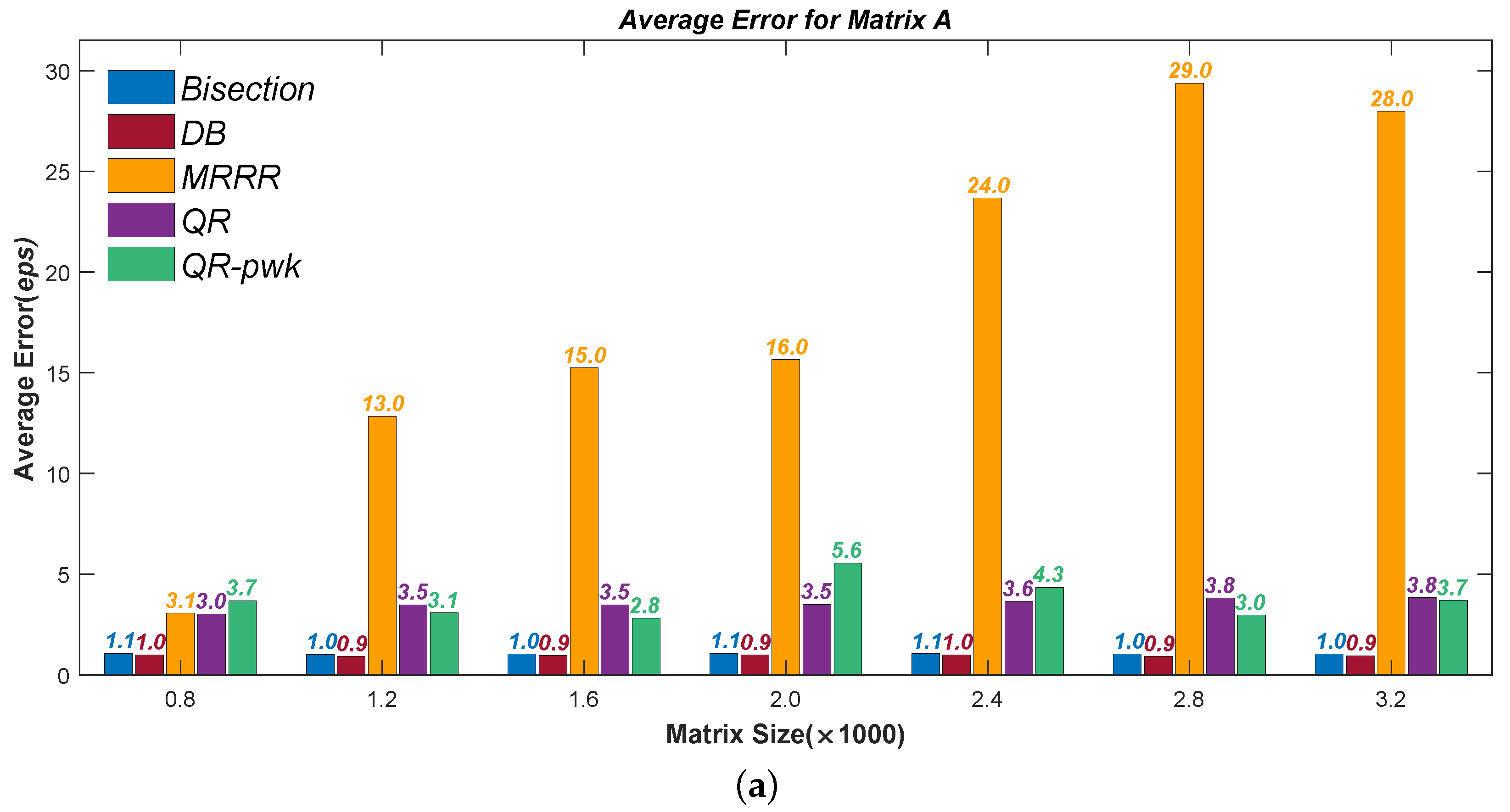
In the following subsections, we present a numerical comparison among the Divisional Bisection algorithm and four other algorithms for solving the ST eigenvalue problem:

1.

Bisection, by calling subroutine ‘dstebz’ from LAPACK in Matlab;

2.

MRRR, by calling subroutine ‘dstegr’ from LAPACK in Matlab;

3.

QR, by calling subroutine ‘dsteqr’ from LAPACK in Matlab;

4.

PWK version of QR (which would be denoted by QR-pwk in the figures), by calling subroutine ‘dsterf’ from LAPACK in Matlab.

We use the following sets of test $n\times n$ matrices:

1.

Matrix A:

$$\mathrm{Matrix}\mathrm{A}=\mathrm{tridiagonal}\left[\begin{array}{ccccccc}& 1& & 1& & \cdots & 1\\ 2& & 2& & \cdots & & & 2\\ & 1& & 1& & \cdots & 1\end{array}\right],$$

i.e., the Toeplitz matrix [1,2,1] to test the accuracy and efficiency, which has ${\lambda }_i=2-2cos(i\pi /(n+1))$;

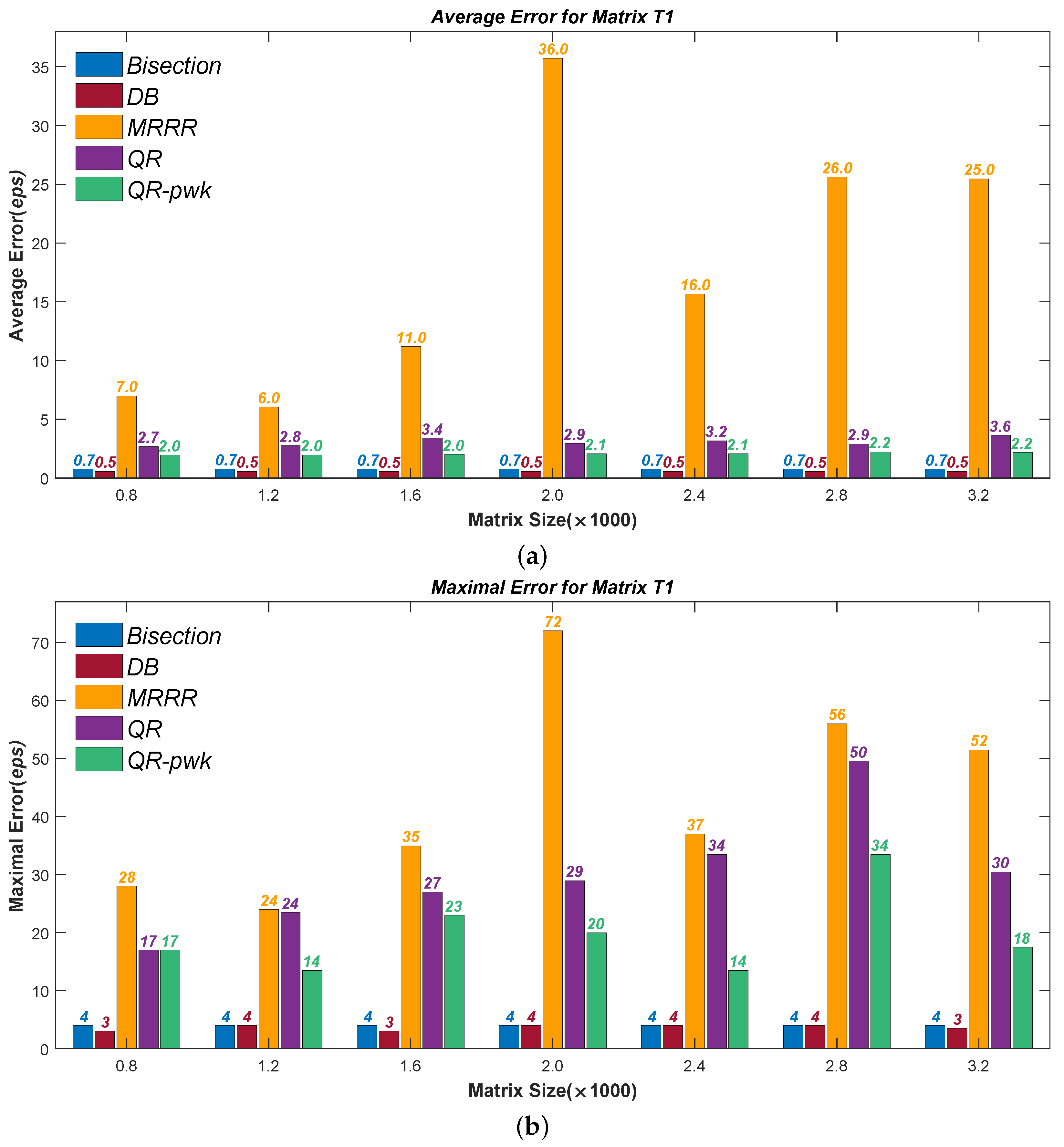
2.

Matrix T1:

$$\mathrm{Matrix}\mathrm{T}1=\mathrm{tridiagonal}\left[\begin{array}{ccccccc}& 1& & 1& & \cdots & 1\\ 1& & 0& & \cdots & & & 0\\ & 1& & 1& & \cdots & 1\end{array}\right],$$

to test the accuracy and efficiency, which has ${\lambda }_i=-2cos(2i\pi /(2n+1))$. Matrix T1 is from [45], as well as the following Matrix T2 and T3;

3.

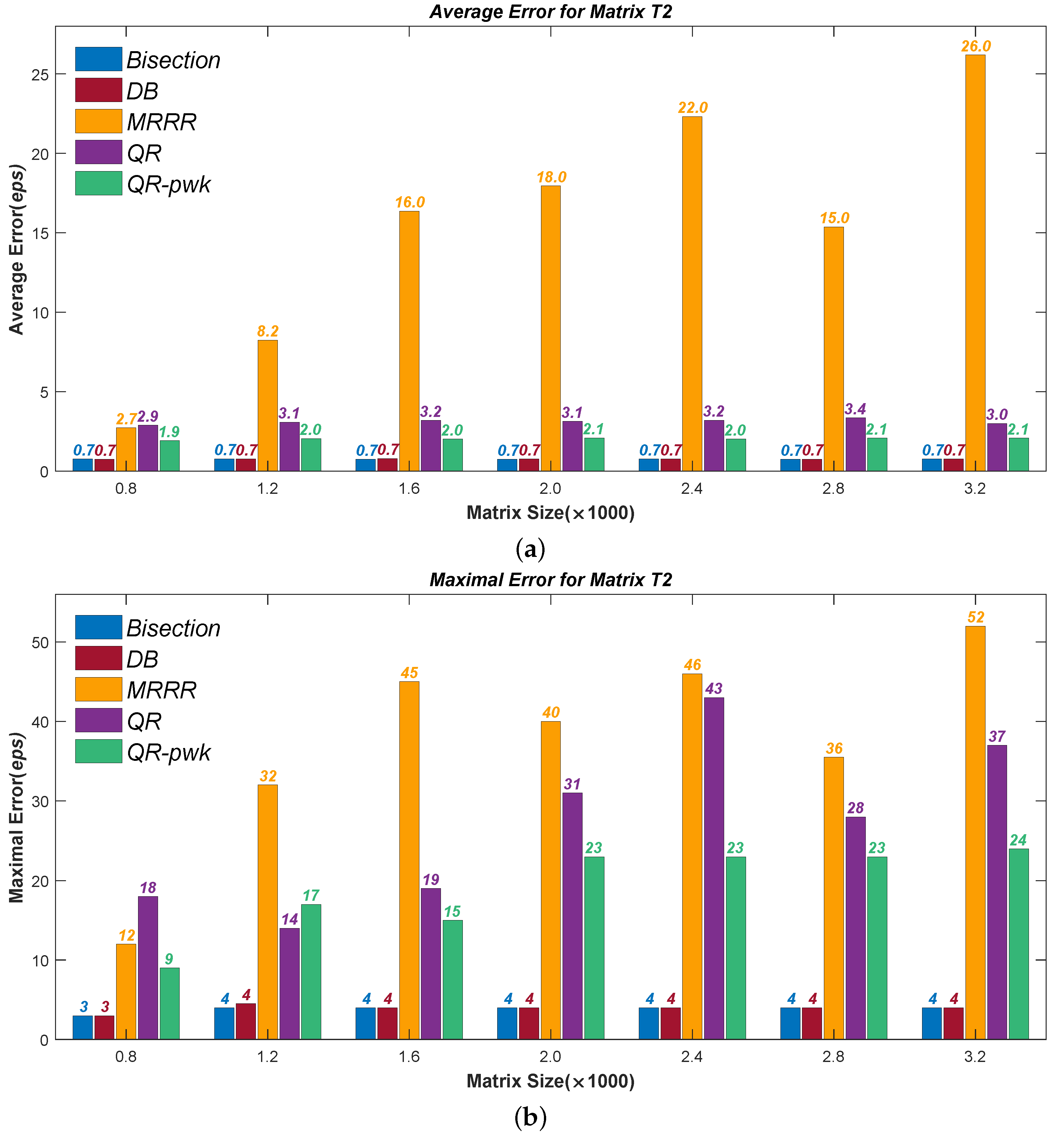
Matrix T2 [45]:

$$\mathrm{Matrix}\mathrm{T}2=\mathrm{tridiagonal}\left[\begin{array}{ccccccc}& 1& & 1& & \cdots & 1\\ 1& & 0& & \cdots & & & 1\\ & 1& & 1& & \cdots & 1\end{array}\right],$$

to test the accuracy and efficiency, which has ${\lambda }_i=-2cos(i\pi /n)$;

4.

Matrix T3 [45]:

$$\mathrm{Matrix}\mathrm{T}3=\mathrm{tridiagonal}\left[\begin{array}{ccccccc}& 1& & 1& & \cdots & 1\\ 1& & 0& & \cdots & & & -1\\ & 1& & 1& & \cdots & 1\end{array}\right],$$

to test the accuracy and efficiency, which has ${\lambda }_i=2cos((2i-1)\pi /\left(2n\right))$;

5.

Matrix W [12,46], which has the ith diagonal component equal to $\left|\right(n+1)/2-i|$(n is odd) and all off-diagonal components equal to 1, to test the efficiency only as its exact eigenvalues are not accessible;

6.

Random Matrix with both diagonal and off-diagonal elements being uniformly distributed random numbers in [−1,1] to test the efficiency only as its exact eigenvalues are not accessible.

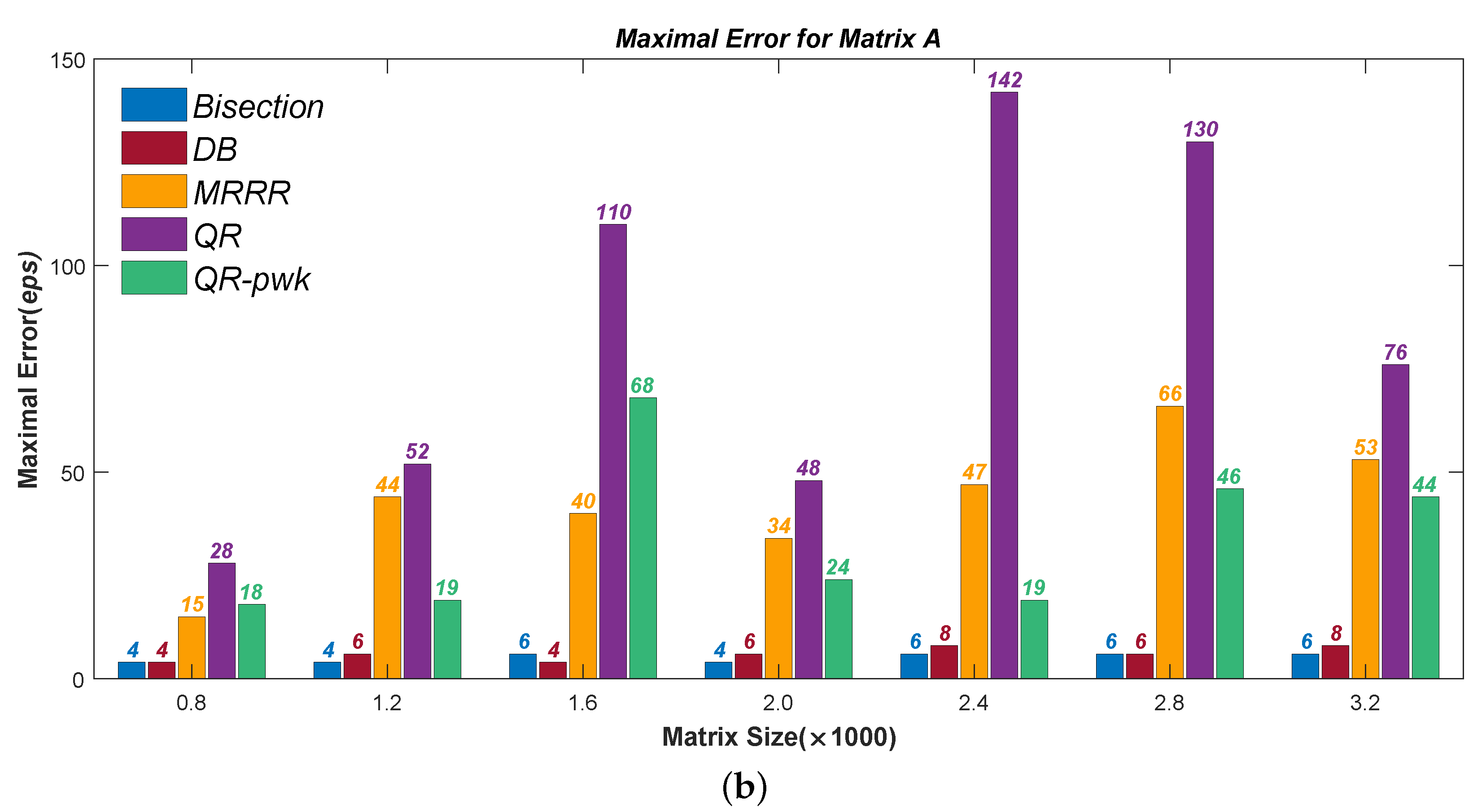
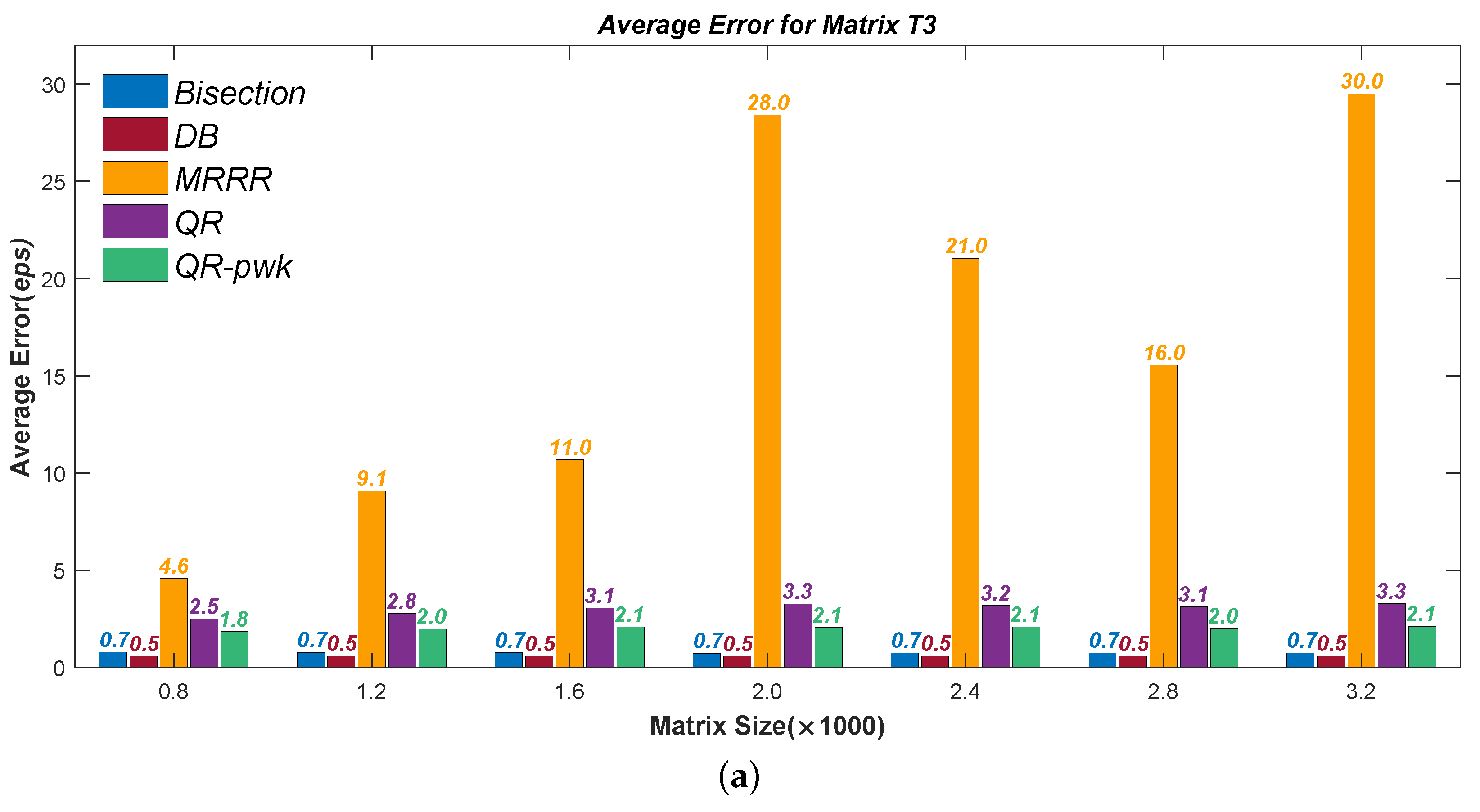
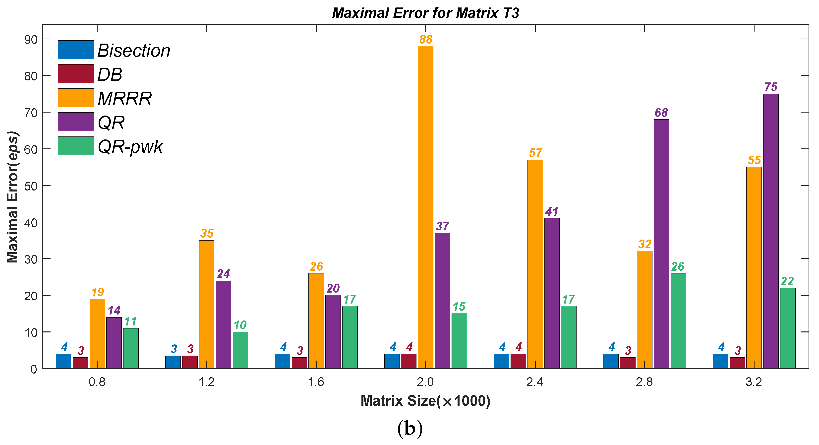
Figure 1, Figure 2, Figure 3 and Figure 4 present the test results of accuracy, where the Average Errors denote the means of errors of all the calculated eigenvalues and the Maximal Errors denote the maximum. Seven different sizes are used, from $800\times 800$ to $3200\times 3200$. All errors have been divided by the machine precision $eps$ for clarity. It can be seen that the new Divisional Bisection algorithm has the best accuracy as well as the Bisection method, considerably higher than the others.

5.3. Efficiency Test for Computing all the Eigenvalues

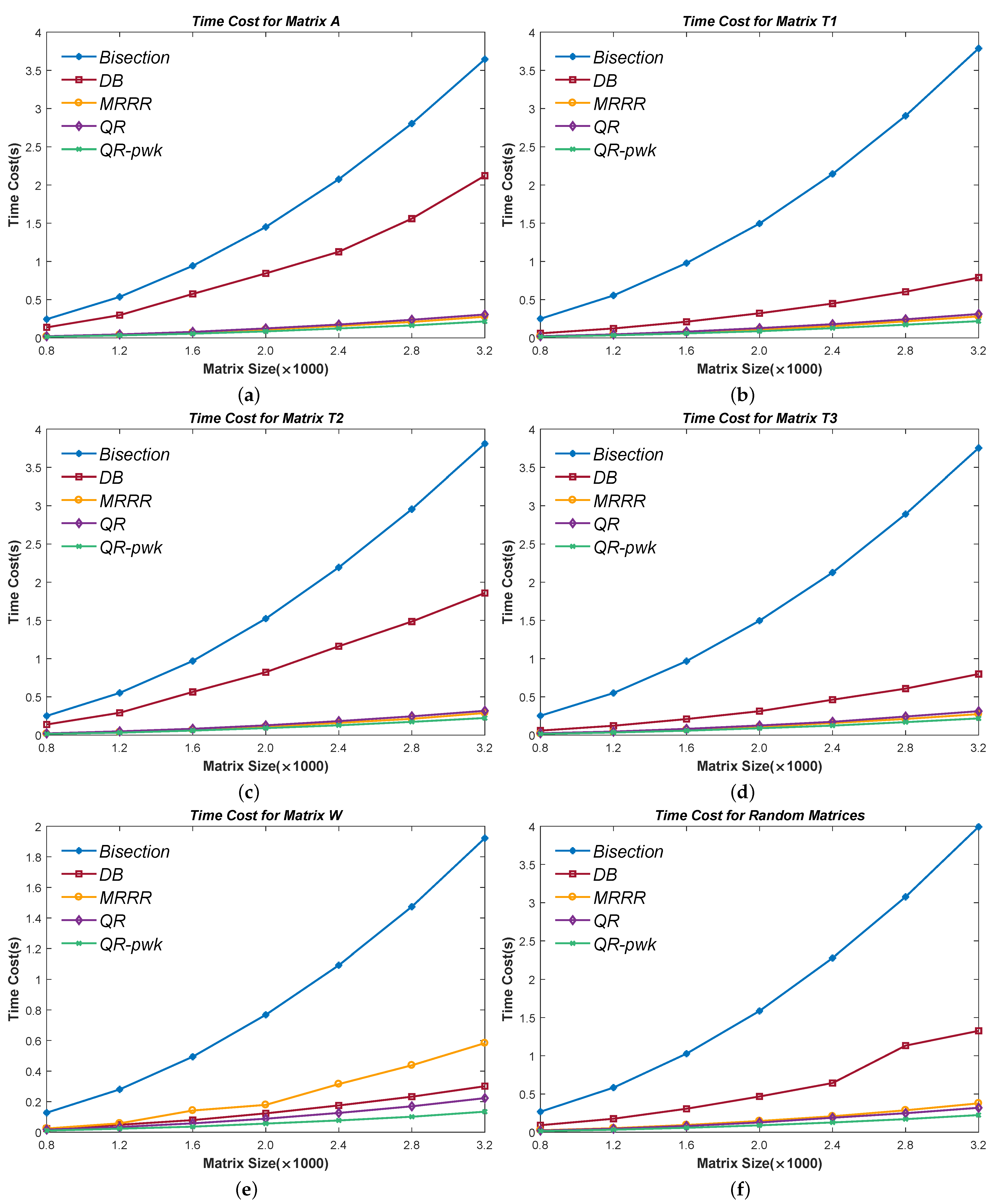
Figure 5 presents the test results of time cost. Seven different sizes are used, from $800\times 800$ to $3200\times 3200$. Note that the results of the Random Matrix of each size are the mean data of 20 tests. Therefore, we use the plural form in the figures.

When the eigenvalues clutter, as in Matrix W, the Divisional Bisection method improves the Bisection method by about $70\%$. Such a good result can also be in Matrix T1 and Matrix T3. However, the improvement is less than $50\%$ in Matrix A and Matrix T2. The reason is their submatrices have close eigenvalues to the global one but are not equal in finite precision arithmetic. For example, the sub-eigenvalues give an interval for Algorithm 6 and have an upper or lower bound that has a distance between ${\lambda }_i$ less than $5\times {10}^{-14}$. The ‘fzero’ scheme uses the linear interpolation to accelerate convergence; such a bound produces poor slopes during the linear interpolation process. As a consequence, more iterations are needed to guarantee convergence, which finally results in the efficiency loss of the Divisional Bisection method. Recall that Algorithm 7 is for checking similar situations. However, a distance of $5\times {10}^{-14}$ could not be detected, because it does not meet the conditions of Theorem 4.

Nevertheless, we are not pessimistic about the Divisional Bisection method. First, it still improves more than $35\%$ in such cases and performs well for Random Matrices. Secondly, the ‘fzero’ scheme is not a prerequisite or non-replaceable in our method, which could be modified or substituted by a more powerful competitor in future follow-up studies.

5.4. Efficiency Test for Computing a Part of the Eigenvalues

All along, the Bisection method undertakes the task of computing a part of eigenvalues, especially when the size of the matrix is large. When Algorithm 5 obtains all the sub-eigenvalues, as shown in lines 2–11 in Algorithm 5, it is an easy task to calculate any parts of ${\lambda }_i$’s. For example, if eigenvalues in a certain interval are wanted, we can drop the sub-eigenvalues which are outside and substitute $\pm F$, in Algorithm 5 line 2 and line 15, with the upper and lower bounds of the given interval. If $r1$th∼$r2$th eigenvalues are wanted, we need to drop the sub-eigenvalues that are of the order lower than $r1-1$ or higher than $r2$. When $s_{r1-1}$ and $s_{r2}$ are the substitutions of $\pm F$, the problem can be solved.

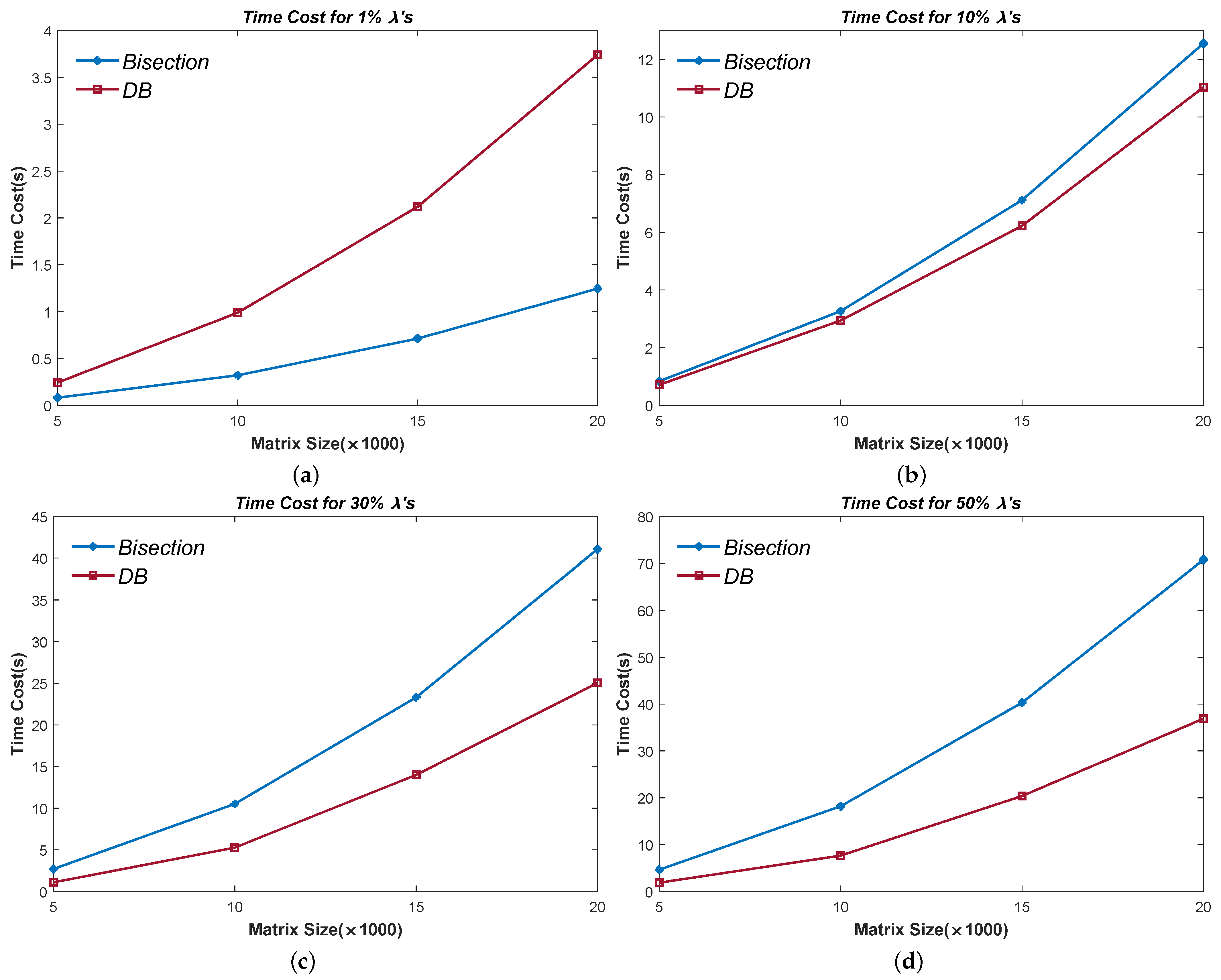
Figure 6 shows the time cost in Random Matrices of four relatively large size, i.e., $5000\times 5000$, 10,000 × 10,000, 15,000 × 15,000, and 20,000 × 20,000. We calculated $1\%$, $10\%$, $30\%$, and $50\%$${\lambda }_i$’s of each size. Note the results are mean data of 40 tests, 20 for computing ${\lambda }_i$’s in a certain interval and 20 for computing ${\lambda }_i$’s in a certain order. Given that there is no evident difference between the test results of calculating ${\lambda }_i$’s in an interval or order, we mixed them for averaging.

The results show that the Divisional Bisection method is not suitable for computing a small group of eigenvalues, despite the matrix being relatively large. We consider $10\%$ as an applicable threshold. Although we can replace the QR method with the Bisection method in Algorithm 5 line 3, which could avoid the calculation of all the sub-eigenvalues, the result seems even worse. As the matrix size increases, the efficiency disadvantage of the Bisection method becomes increasingly severe, which could ignore only a quite small number of wanted ${\lambda }_i$, for example, $0.1\%$. In this case, the ‘fzero’ loops (line 12 to line 24 in Algorithm 5) become a heavy burden to the Divisional Bisection method. Therefore, we insist on using the PWK version of the QR method in Algorithm 5.

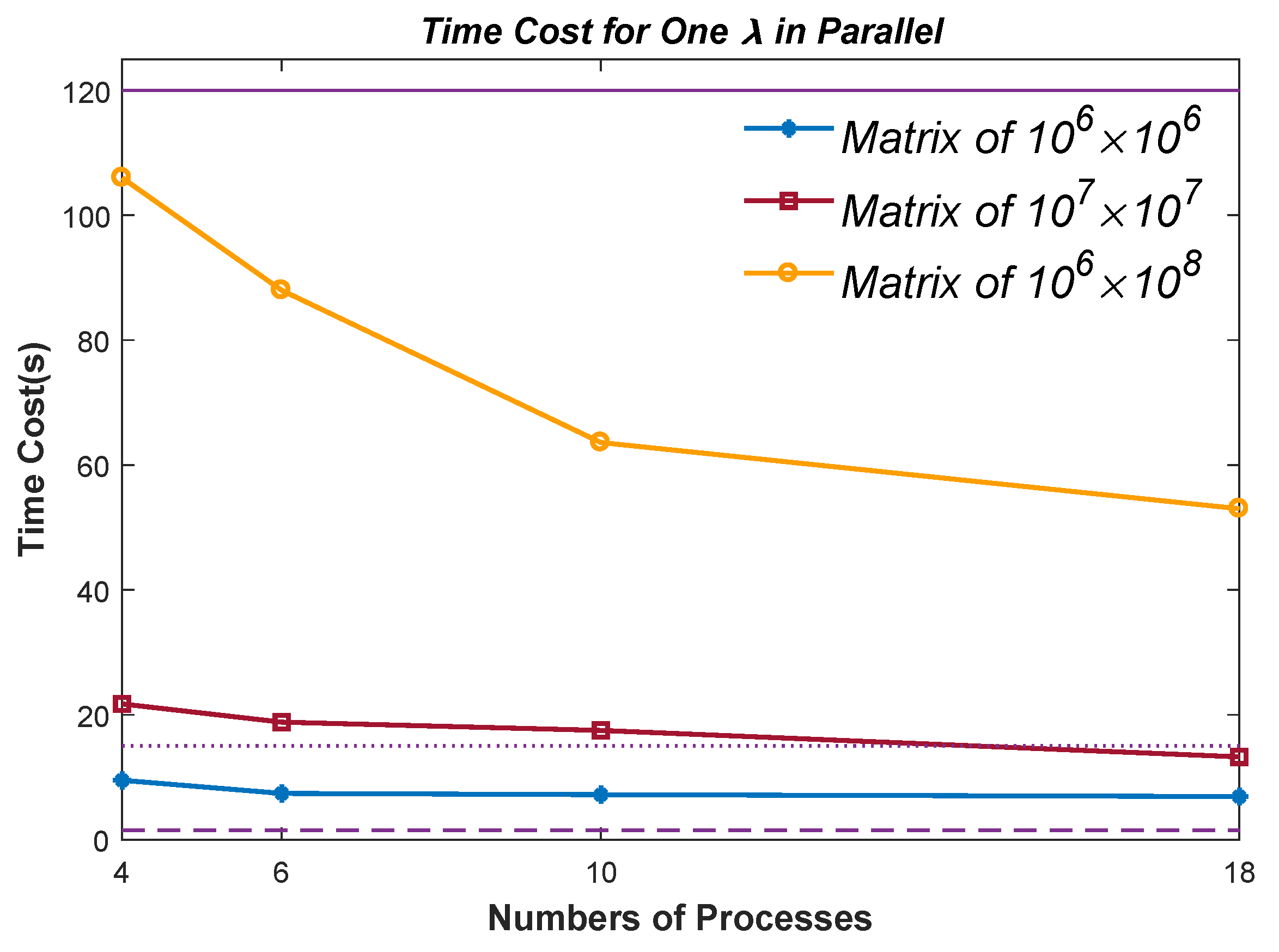
We now consider the situation of calculating one $\lambda$ in parallel. The problem also arises when the number of wanted $\lambda$ is less than the number of CPU cores or not divisible by it. Algorithm 4 solves the problem and makes it available for computing with any number of CPU cores. Of course, the need to compute an eigenvalue in parallel must occur in a very large matrix. Therefore, we use three Random Matrices with sizes of ${10}^6\times {10}^6$, ${10}^7\times {10}^7$, and ${10}^8\times {10}^8$ for the test of parallel efficiency. The results, presented in Figure 7, were collected on an Intel Xeon(R) Core E5-2687 3.1-GHz CPU and 256-GB RAM machine, which has 20 CPU cores. Note that the results are mean data of 20 tests.

The three purple horizontal lines in Figure 7 denote the time cost of the serial Bisection algorithm. Specifically, the top one denotes the time cost for ${10}^8\times {10}^8$ Random Matrices, the middle ${10}^7\times {10}^7$, and the bottom ${10}^6\times {10}^6$. The parallel efficiency is unsatisfactory, especially for the ${10}^7\times {10}^7$ and ${10}^6\times {10}^6$ Random Matrices, which are even worse than the serial Bisection algorithm. The reason is that Matlab is not available for multi-threaded computation. Instead, we run the codes in multi-processes. The task of copying inputs and distributing them to the processes takes up the vast majority of the time. The script time consumption analysis tool in Matlab confirms our point, which shows at least $75\%$ time was consumed during copying and distributing. Therefore, we would focus on the version written in C or Fortran of the Divisional Bisection algorithm in future follow-up studies. Nevertheless, Figure 7 verifies the feasibility of Algorithm 4, which to our knowledge is the only algorithm that works in parallel for computing any one ST eigenvalue. This paper also focuses on the serial version.

6. Conclusions

In this paper, a novel $O\left(n^2\right)$ Divisional Bisection method is given for the ST eigenvalue problem by Algorithms 4 and 5. When computing all eigenvalues, the results show that the time cost is reduced by more than 35–70% on serial machines compared to the Bisection algorithm. In addition,

1.

The algorithms are easy to implement fully in parallel;

2.

By Algorithm 4, even one eigenvalue can be calculated in parallel and distributed on any number of CPU cores;

3.

As with the Bisection algorithm, it is flexible to set the expected accuracy and the computing error archives machine precision;

4.

By Algorithm 4, it is practicable to calculate a single eigenvalue of any order;

5.

Combining Algorithms 4 and 5, it is practicable to calculate eigenvalues in any interval in parallel or any orders.

The Divisional Bisection method offers a novel idea for solving the ST eigenvalue problem and a new choice, especially for readers who care about an algorithm of good parallelization, flexibility, and warranted accuracy.