Lie Symmetry Analysis and Conservation Laws of the Axially Loaded Euler Beam

Abstract

By applying the Lie symmetry method, group-invariant solutions are constructed for axially loaded Euler beams. The corresponding mathematical models of the beams are formulated. After introducing the infinitesimal transformations, the determining equations of Lie symmetry are proposed via Lie point transformations acting on the original equations. The infinitesimal generators of symmetries of the systems are presented with Maple. The corresponding vector fields are given to span the subalgebra of the systems. Conserved vectors are derived by using two methods, namely, the multipliers method and Noether’s theorem. Noether conserved quantities are obtained using the structure equation, satisfied by the gauge functions. The fluxes of the conservation laws could also be proposed with the multipliers. The relations between them are discussed. Furthermore, the original equations of the systems could be transformed into ODEs and the exact explicit solutions are provided.

1. Introduction

In geometrical terms, the Lie symmetry group is a fundamental coordinate-free structure of differential equations. In the field of analytical mechanics, the Lie group is applied to dynamical systems expressed by both ordinary differential equations (ODEs) and partial differential equations (PDEs). In particular, the use and importance of symmetries and conservation laws for constrained ordinary differential systems have been studied deeply in the last few decades [1,2,3,4,5,6,7]. A considerable number of mathematicians have used PDEs to describe many complex nonlinear phenomena in the fields of electromagnetism, fluid mechanics, astrophysics, condensed matter physics, etc. These PDE mathematical models are significant because these equations describe multiple behaviors in various sciences. The Lie symmetry group of a system of differential equations can transform solutions of the system into other solutions. This method is the most powerful, general and systematic approach for finding exact solutions for these PDEs. Sil and Rajasekhar performed the classification of nonlocal symmetries and obtained some implicit solutions and one arbitrary family of solutions for the system of nonlinear partial differential equations [8]. Ref. [9] concerned the generalized cylindrical KdV equation and provided exact solutions in a general case. Yadav and Arora investigated the (3 + 1)-dimensional nonlinear wave equation in a liquid with gas bubbles and obtained the exact solutions of the (3 + 1)-dimensional nonlinear wave equation [10]. The Lie symmetry method can also be used in fields of mathematical physics and engineering sciences, such as fluid dynamics [11,12], fluid engineering [13], geophysics [14], etc. Symmetry reductions and group-invariant solutions can be obtained while the Lie group analysis is performed for nonlinear equations. The systematic methods were proposed in [2,15] and the references therein. The Lie group classification of these equations was performed, and Lie point symmetries were presented via variational principles.

There are several analytical methods for finding the solutions to these kinds of equations, such as the Noether theorem, the extended Noether theorem and the multipliers method. For variational symmetries, the Lagrangians and symmetries are used to derive conservation laws in Lagrangian variables by means of Noether’s theorem. The Noether theorem, when applied to differential equation systems, has a Lagrangian formulation for a suitable Lagrangian function. Some new results and details can be found in Bluman, Cheviakov and Anco’s book [16] (see references therein). However, there are differential equations that do not admit to a Lagrangian formulation. In such cases, the extended Noether theorem can construct conservation laws of Euler–Lagrange-type equations via Noether-type symmetry operators associated with partial Lagrangians. Anco and Wang obtained an explicit formula to find symmetry recursion operators for partial differential equations from new results connecting variational integrating factors and nonvariational symmetries [17]. In addition, the multipliers method is also a way of obtaining divergence conservation laws in cases when a system does not directly have a usual Lagrangian (see [16] and the references therein). For these three methods, the Noether theorem is the main way of obtaining the conservation laws of variational symmetries, and the extended Noether theorem and the multipliers method can propose the laws, although these systems are nonvariational.

The mathematical model of the axially loaded Euler beam is a fourth-order PDE. Studies of the Euler beam are the basis of analytical solutions, the dynamic response and applications of models of various beams [18,19]. For fourth-order beam models in the literature up to the year 2000, the Lie group approach to the beam has been studied in analytical solutions using symmetry reduction [20,21,22] and integrability through symmetries [23,24,25]. In Ref. [22], closed solutions of equations describing nonuniform axially loaded beams were obtained using the Lie symmetry method. The solutions were directly obtained from the simpler form of the governing equation, which was based on the preferred coordinate transformation. The current paper focuses on symmetry reduction and conservation laws. Our model is a special case of a nonuniform beam. The symmetry reduction for the systems is the subversion of more general solutions given in [22]. However, different from the former, the conservation laws and relations between symmetries and conserved quantities are discussed in this paper. For axially loaded beams, these conserved quantities are of major importance and can reveal the inner physical meanings of dynamical systems. Ref. [26] also constructed the exact solutions of fourth-order diffusion equations by using the Lie symmetry method. Although it did not refer to the conservation laws, it was of significant reference for the symmetry reduction of the fourth-order Euler beam.

The exact solution of a fourth-order partial differential equation is an open question. Some models even have no closed solutions. The Lie group method can reduce the order of the PDE or transform the PDE into ODEs by using the coordinate transformations. Reduced systems of determining equations are normally much simpler and are integrated automatically or even by hand. Therefore, solutions of the systems can be obtained easily using the Lie group method. The Lie group can be simpler than the classic way of obtaining the exact solutions.

In previous works on the axially loaded beam, researchers focused on searching closed-form solutions using Lie symmetry reductions. One may work out the Lie determining equations of the systems by hand. However, with an increasing degree of equations, construction by hand becomes harder and harder, and even impossible. In this paper, we applied the Maple procedures to the simpler beams model and produced a simpler way to solve it. For the mathematical model of the axially loaded beam, some references studied the conservation laws using the multipliers method. However, the relations between the symmetry vector fields and the conservation laws did not receive much consideration. In this paper, we gave forms of conserved quantities. The relations between the Noether symmetry method and the multipliers method are also proposed. Although this model is simpler, it might propose a way of studying the relations between symmetries and conservation laws for flexible mathematical models, such as nonuniform Euler beams, axially moving systems, etc.

Based on the symmetry reduction theory, we also reduce the PDE of the beam to ODE forms and produce the corresponding exact solutions in this paper. In particular, in terms of finding conserved quantities, we derive the conservation laws directly from the original fourth partial equation of the system. It is different from those of previous works [21,23,24,25]. In those previous works, the conservation laws of the reduced Equation (ODE) rather than the system itself were discussed. Although reference [23] obtained the conservation laws from an original equation, it considered the case of the centripetal force distribution of the beam, which was the scalar lower-order ordinary difference equation. Therefore, we directly derive the conservation laws of the original equation of the fourth axially loaded Euler beam by using two different methods: the Noether theorem and the multipliers method. Some of these conservation laws have the same form, but some of them do not. They all reveal the inner physical properties of the system under certain conditions.

This paper is organized as follows: The introduction is presented in the first section. In Section 2, the kinetic analysis and problem formulations are reviewed and the equation is considered. In Section 3, the Lie symmetry group of the axially loaded Euler beam is presented. In Section 4, the conservation laws for the axially loaded Euler beam are obtained by using the Noether theorem and the multipliers method. In Section 5, we consider the symmetry reductions by using the Lie group method and provide exact explicit solutions. Finally, the conclusions of this paper are presented in the last section.

2. The Dynamic Equation of the Axially Loaded Euler Beam

Consider that a uniform beam has small-amplitude vibrations in the transverse directions between two boundaries. It is loaded by an axial force P₀. The large deformation of the rod is not considered. The span between the two boundaries is denoted by l. The fixed axial coordinate x measures the distance from the left boundary. 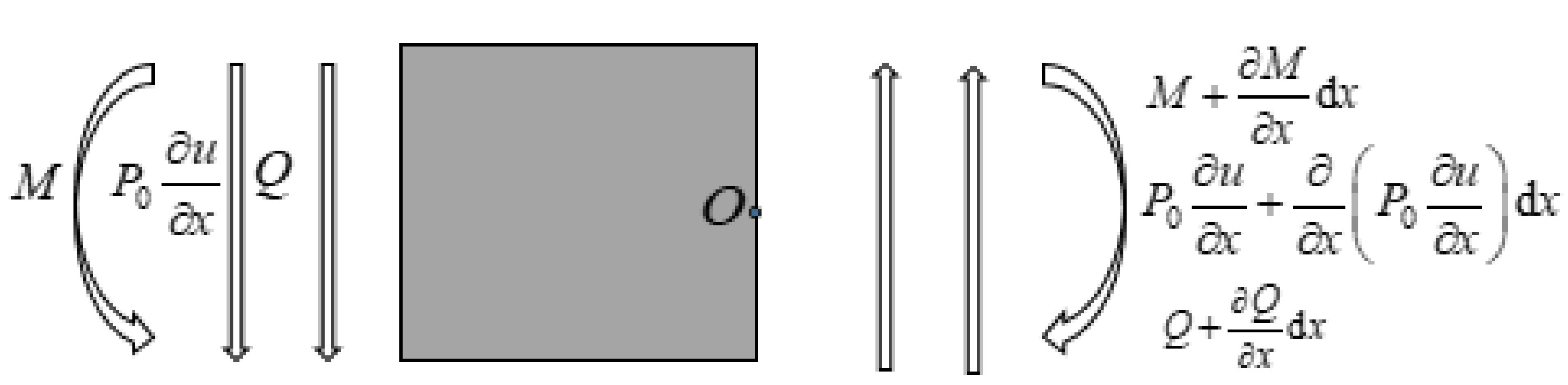Only the bending vibration described by the transverse displacement u (x, t) is considered, where u (x, t) is the transversal displacement at time t and position x. The analysis diagram for the microsection dx with the transverse shear force Q (x, t) and the bending moment M (x, t) is shown in Figure 1.

The force balance equation in the transverse directions is

$$\rho A\mathrm{d}x\frac{{\partial }^{2}u}{\partial t^2}-P_0\frac{{\partial }^{2}u}{\partial x^2}\mathrm{d}x-\frac{\partial Q}{\partial x}\mathrm{d}x=0,$$

(1)

in which $\rho$ is the linear mass density, A is the area of the cross-section of the beam. The torque equilibrium equation is

$$Q\mathrm{d}x-\frac{\partial M}{\partial x}\mathrm{d}x=0.$$

(2)

For a slender beam, the linear moment–curvature relationship is

$$M=-EI\frac{{\partial }^{2}u}{\partial x^2},$$

(3)

in which E is the elastic modulus, I is the area moment of inertia and EI is the flexural rigidity. These equations can be investigated algebraically for E, I, $\rho$ and P₀ as some given constants or functions. From Equations (1) to (3), the transverse motion of the axially loaded beam is

$$EI\frac{{\partial }^{4}u}{\partial x^4}-P_0\frac{{\partial }^{2}u}{\partial x^2}+\rho A\frac{{\partial }^{2}u}{\partial t^2}=0.$$

(4)

Equation (4) can be cast into the dimensionless form

$$u_{xxxx}+u_{tt}-\mathsf{\Phi }{u}_{xx}=0,$$

(5)

where the subscript x or t denotes the partial differentiation with respect to x or t, and the dimensionless variables and parameters are

$$u\leftrightarrow \frac{u}{l},\hspace{1em}t\leftrightarrow t\sqrt{\frac{EI}{\rho A{l}^4}},x\leftrightarrow \frac{x}{l},\hspace{1em}\mathsf{\Phi }\leftrightarrow \frac{P_0{l}^2}{EI}.$$

In this paper, the Lie symmetry and conserved quantities of the transverse vibration of the axially loaded beam were the main focus.

3. Lie Symmetry of the Axially Loaded Euler Beam

Lie symmetry is a kind of invariance of differential equations under infinitesimal transformations of coordinates. The Lie algebra of the symmetry group is realized using vector fields and prolonged vector fields. Readers can consult the proper references, e.g., Refs. [2,3,15] or [17], for the general method of Lie symmetry of differential equations. Readers can also read the details in Appendix A.

Based on the general method of Lie symmetry in Appendix A, the application of the Lie symmetry analysis of the axially loaded beam (5) is as follows.

For the Equation (5), $M=R^2\times R$, that is $x_1=t,x_2=x,u^1=u$ and the fourth prolongation of the vector field X can be constructed as

$$pr{X}_i^{(4)}=X_i+{\eta }^{tt}\frac{\partial }{\partial u_{tt}}+{\eta }^{xx}\frac{\partial }{\partial u_{xx}}+{\eta }^{xxxx}\frac{\partial }{\partial u_{xxxx}},$$

(6)

where

$$\begin{array}{l}{\eta }^t=D_t(\eta )-u_x{D}_t(\xi )-u_t{D}_t(\tau ),{\eta }^{tt}=D_t({\eta }^t)-u_{xt}{D}_t(\xi )-u_{tt}{D}_t(\tau ),\\ {\eta }^x=D_x(\eta )-u_x{D}_x(\xi )-u_t{D}_x(\tau ),{\eta }^{xx}=D_x({\eta }^x)-u_{xx}{D}_x(\xi )-u_{xt}{D}_x(\tau ),\\ {\eta }^{xxx}=D_x({\eta }^{xx})-u_{xxx}{D}_x(\xi )-u_{xxt}{D}_x(\tau ),{\eta }^{xxxx}=D_x({\eta }^{xxx})-u_{xxxx}{D}_x(\xi )-u_{xxxt}{D}_x(\tau ).\end{array}$$

By introducing the infinitesimal transformations and the extended vector (6), the invariance of Equation (5) under the infinitesimal transformations leads to the satisfaction of the determining equation

$$pr{X}_{}^{(4)}(u_{xxxx}+u_{tt}-\mathsf{\Phi }{u}_{xx})\left|{}_{u_{xxxx}+u_{tt}-\mathsf{\Phi }{u}_{xx}=0}\right.=0.$$

(7)

Suppose a beam with a square section has a side length $a=0.01 \mathrm{m}$, a modulus of elasticity $E=2.1\times {10}^{11} \mathrm{Pa}$ and a density $\rho =7850 \mathrm{kg}/{\mathrm{m}}^3$. Let the tension be $P_0=1750 \mathrm{N}$ and the cross-sectional area of the square section of the beam be $A=1\times {10}^{-4} {\mathrm{m}}^2$; therefore, coefficient $\mathsf{\Phi }=10$. The determining Equation (7), thus, involves t, x and u, as well as ${\xi }_1,{\xi }_2$ and $\eta$ and their partial derivatives with respect to t and x. This results in solving a large number of equations for the coefficient functions ${\xi }_1,{\xi }_2$ and $\eta$ for the infinitesimal generator. In most instances, these determining equations can be solved with the elementary method, and the general solution determines the most general infinitesimal symmetry of the system. In this paper, the symmetry operators were obtained in Maple. In general, the low-order differential equations can be solved with the determine() provided by liesymm, an embedded software package in the Maple system [27]. The solution of symmetric equations of higher-order nonlinear partial differential equations can be obtained by means of some standard software packages, such as PDEtools [28], SADE [29], GeM [30], etc.

Equating the coefficients of the various monomials in the partial derivatives of u, such as $[u_t,u_{ttt},u_{tttt},u_{tttx},u_{ttx},u_{ttxx},u_{tx},u_{txx},u_{txxx},u_x,u_{xx},u_{xxx},u_{xxxx}]$, the determining equations for the symmetry group system (5) can be obtained in the Maple system [28]. After simplifying and reducing, the overdetermined system of symmetry determining equations can be rewritten as

$$\begin{array}{l}{\eta }_{xxxx}=10{\eta }_{xx}-{\eta }_{tt},\hspace{1em}{\eta }_{ux}=0,\hspace{1em}{\eta }_{ut}=0,\hspace{1em}{\eta }_{uu}=0,\\ {\xi }_{1,x}^{}=0,\hspace{1em}{\xi }_{2,x}^{}=0,\hspace{1em}{\xi }_{1,t}^{}=0,\hspace{1em}{\xi }_{2,t}^{}=0,\hspace{1em}{\xi }_{1,u}^{}=0,\hspace{1em}{\xi }_{2,u}^{}=0.\end{array}$$

(8)

For the generators ${\xi }_{1,x}=0,{\xi }_{1,t}=0$ and ${\xi }_{1,u}=0$ we had ${\xi }_1=c_1$; for ${\xi }_{2,x}=0$, ${\xi }_{2,t}=0$ and ${\xi }_{2,u}=0$ we had ${\xi }_2=c_2$; and the conditions ${\eta }_{ux}=0,{\eta }_{ut}=0$ and ${\eta }_{uu}=0$ produced $\eta =c_{3}u+V\left(t, x\right)$. All coefficient functions of the infinitesimal generator were obtained as follows:

$${\xi }_1=c_1,\hspace{1em}{\xi }_2=c_2,\hspace{1em}\eta =c_{3}u+\varsigma \left(t,x\right).$$

Therefore, the infinitesimal generators admitted by the Euler beam equation of motion had the following form:

$$X_i=c_1{\partial }_x+c_2{\partial }_t+\left(c_{3}u+\varsigma \left(t,x\right)\right){\partial }_u,$$

where $c_1,c_2$ and $c_3$ are arbitrary constants and $\varsigma \left(t, x\right)$ satisfies ${\varsigma }_{xxxx}+{\varsigma }_{tt}-10{\varsigma }_{xx}=0$ for Equation (5). The solutions of (8) are given by the span of the operators

$$X_1={\partial }_x,$$

(9)

$$X_2={\partial }_t,$$

(10)

$$X_3=u{\partial }_u,$$

(11)

and the infinite-dimensional subalgebra

$$X_{\varsigma }=\varsigma (x,t){\partial }_u,$$

(12)

where $\varsigma$ is an arbitrary solution of the equation of the axially loaded beam, i.e., satisfying ${\varsigma }_{xxxx}+{\varsigma }_{tt}-10{\varsigma }_{xx}=0$. These are the elementary symmetries, which exist for any linear PDE.

It is easy to check that $\left\{X_1,X_2,X_3\right\}$ is closed under the Lie bracket. For Equation (5), we had

$$\begin{array}{l}[X_1,X_1]=[X_2,X_2]=[X_3,X_3],\\ [X_1,X_2]=-[X_2,X_1]=[X_1,X_3]=-[X_3,X_1]=[X_2,X_3]=-[X_3,X_2]=0,\end{array}$$

and

$$\begin{gathered} [X_1,X_{\varsigma }]=-[X_{\varsigma },X_1]={\varsigma }_x{\partial }_u=X_{{\varsigma }_x},\hspace{1em}[X_2,X_{\varsigma }]=-[X_{\varsigma },X_2]={\varsigma }_t{\partial }_u=X_{{\varsigma }_t}, \\ [X_3,X_{\varsigma }]=-[X_{\varsigma },X_3]=-\varsigma {\partial }_u=-X_{\varsigma },\hspace{1em}[X_{\varsigma },X_{\varsigma }]=0. \end{gathered}$$

Therefore, we can see that the generators of the invariant group

$$X_i={\xi }_1(t,x,u)\frac{\partial }{\partial t}+{\xi }_2(t,x,u)\frac{\partial }{\partial x}+\eta (t,x,u)\frac{\partial }{\partial u}$$

of (7) construct an infinite-dimensional Lie algebra, which includes a three-dimensional subalgebra spanned by the basis $\left\{X_1,X_2,X_3\right\}$, respectively.

Furthermore, for equaiton (5), the one-parameter groups $G_i$ generated by $X_i(i=1, 2 ,3)$ are given in the following:

$$\begin{array}{l}{G}_1:\left(x,t,u\right)\to \left(x+\epsilon ,t,u\right),\\ G_2:\left(x,t,u\right)\to \left(x,t+\epsilon ,u\right),\\ G_3:\left(x,t,u\right)\to \left(x,t,e^{\epsilon }u\right),\\ G_{\varsigma }:\left(x,t,u\right)\to \left(x,t,u+\epsilon \varsigma (x,t)\right).\end{array}$$

From the table above, we observed that $G_1$ is a spatial translation, $G_2$ is a time translation and $G_3$ is a scaling of dependent variables.

4. Conservation Laws

Local conservation laws of systems of partial differential equations can mainly apply to the following aspects. Firstly, they can serve as mathematical expressions for fundamental physical principles. Secondly, they can be used in the analysis and stability of systems governed by PDEs. Thirdly, a conserved quantity is an important general structure and it can be used to construct structure-preserving numerical schemes in the development of numerical methods.

There are two main ways to construct conservation laws for general mechanical systems. One is the Noether theorem, and the other is the multipliers method, which is also called the direct method. The Noether theorem is the most well-known systematic method used for self-adjoint (variational) systems [1]. The other is called the direct method (multipliers method), which is a relatively powerful method for constructing local conservation laws. It involves integrations and arbitrary functions. In this paper, the conservation laws of system (5) could be obtained with the Noether theorem and the multipliers method.

4.1. The Noether Theorem

Noether symmetry is an invariance of the Hamilton action under the infinitesimal transformations of coordinates. A Noether symmetry can lead to a conserved quantity according to the Noether theorem. The study of the Noether theorem can be seen in references [2,3,15,17,31]. Readers can also refer to Appendix B. In the following, the Noether theorem was applied directly to the axially loaded beam (5).

The German mathematician Noether proposed the Noether theorem. Therefore, for Equation (5) of the axially loaded beam, the Lagrangian of the system can be

$$L=5u_x^2+u_{xxx}{u}_x+\frac{1}{2}{u}_{xx}^2+\frac{1}{2}u{u}_{tt}.$$

(13)

Lie operators (9) and (10), satisfied with identity (A14) in Appendix B with $B^1=B^2=0$, are strict Noether symmetries. The scaling symmetry (11) does not preserve the action and, hence, is nonvariational, with no corresponding conservation law. It is simple to check that $X_1\left(L\right)+L\left\{D_t\left(1\right)+D_x\left(0\right)\right\}=0$ and $X_2\left(L\right)+L\left\{D_t\left(1\right)+D_x\left(0\right)\right\}=0$, where D is the total differentiation operator. A conserved flow of $T=\left(T^1,T^2\right)$ is a vector along which the conservation law

$$D_t{T}^1+D_x{T}^2=0.$$

(14)

The divergence expressions (A15) corresponding to symmetries (9) and (10) are given by

$$X_1=\frac{\partial }{\partial x}, D_t\left(-\frac{1}{2}{u}_t{u}_x+\frac{1}{2}u{u}_{xt}\right)+D_x\left(5u_x^2-u_{xxx}{u}_x+\frac{1}{2}{u}_{xx}^2-\frac{1}{2}u{u}_{tt}\right)=0,$$

(15)

$$X_2=\frac{\partial }{\partial t},D_t\left(5u_x^2+u_{xxx}{u}_x+\frac{1}{2}{u}_{xx}^2-\frac{1}{2}{u}_t^2\right)+D_x\left(10u_x{u}_t-u_{xxx}{u}_t-u_{xxt}{u}_x\right)=0.$$

(16)

Moreover, Equation (5) is the Euler–Lagrange equation for the Lagrangian

$$L=5u_x^2+\frac{1}{2}{u}_{xx}^2-\frac{1}{2}{u}_t^2.$$

(17)

Operators (9) and (10) are the strict Noether symmetries of the standard Lagrangian (17). The conservation laws are

$$X_1=\frac{\partial }{\partial x}, T^1=u_x{u}_t, T^2=-5u_x^2-\frac{1}{2}{u}_t^2+u_x{u}_{xxx}-\frac{1}{2}{u}_{xx}^2,$$

(18)

$$X_2=\frac{\partial }{\partial t},\hspace{1em}{T}^1=L+u_t^2=5u_x^2+\frac{1}{2}{u}_{xx}^2+\frac{1}{2}{u}_t^2,\hspace{1em}{T}^2=-10u_x^2+u_x{u}_{xx}-u_{xx}^2.$$

(19)

For the axially loaded Euler beam, generator $X={\partial }_t$ generates the time translation group G₂, and conservation laws (16) and (19) correspond to the generalized energy for each Lagrangian function. The invariance of the spatial transformation generator $X={\partial }_x$ implies the generalized momentums (15) and (18). With $\psi =u_x$ representing the rotation of the cross-section of the beam, $\overline{M}=-u_{xx}$ denoting the bending moment for the dimensionless form (5), $\overline{Q}={\overline{M}}_x=-u_{xxx}$ denoting the transverse shear force and $\overline{H}=u_x{u}_t$ denoting the wave momentum, the resulting conservation law (15) was found to be

$$D_t\left(-\frac{1}{2}\overline{H}-\frac{1}{2}u\overline{M}\right)+D_x\left(5{\psi }^2-Q\psi +\frac{1}{2}{M}^2-\frac{1}{2}u{u}_{tt}\right)=0.$$

(20)

Expressions (16), (18) and (19) can also be described in the same way. In this point, the conservation laws can also show various balances of bending moment, shear force and loading.

4.2. The Multipliers Method

According to the direct method, one seeks multipliers, such that the linear combination of PDEs of a given system with these multipliers yields a divergence expression. Once local conservation law multipliers have been found, one needs to reconstruct the fluxes of the conservation laws. The study of the multipliers method can be seen in [2,16] and the references therein. The method is also presented in Appendix C. In the following, the multipliers method was applied directly to the axially loaded beam (5).

For Equation (5), the form of the multiplier is $\mathsf{\Lambda }[\mathit{U}]$. The determining Equations (A19) in Appendix C yield the multipliers ${\mathsf{\Lambda }}^{(1)}=u_x$ and ${\mathsf{\Lambda }}^{(2)}=u_{xxx}$. We now determined the corresponding density–flux pairs.

For the multiplier ${\mathsf{\Lambda }}^{(1)}=u_x$, one obviously has

$${\mathsf{\Lambda }}_{\sigma }[\mathit{U}]F_{\alpha }[\mathit{U}]\equiv u_x\left(D_t[u_t]+D_x[u_{xxx}-u_x]\right),$$

(21)

since Equation (5) is in the divergence form as it stands

$$D_t\left(-\frac{u{u}_{tx}}{2}+\frac{u_t{u}_x}{2}\right)+D_x\left(-5u_x^2+u_{xxx}{u}_x-\frac{u_{xx}^2}{2}+\frac{u{u}_{tt}}{2}\right)=0.$$

(22)

Similarly, for the multiplier ${\mathsf{\Lambda }}^{(2)}=u_{xxx}$, one finds the corresponding conservation law

$$D_t\left(-\frac{u{u}_{txxx}}{2}+\frac{u_t{u}_{xxx}}{2}\right)+D_x\left(\frac{u_{xxx}^2}{2}+\frac{u{u}_{ttxx}}{2}-\frac{u_x{u}_{ttx}}{2}+\frac{u_{xx}{u}_{tt}}{2}-5u_{xx}^2\right)=0.$$

(23)

The solution ${\mathsf{\Lambda }}^{(}{}^{\upsilon )}=\upsilon \left(x,t\right),\xi \left(t,x,u\right)=0$, where υ satisfies ${\upsilon }_{xxxx}+{\upsilon }_{tt}-10{\upsilon }_{xx}=0$, produces linear conservation laws, which exist for any linear PDE.

As mentioned in Refs. [2,32,33], two conserved densities T may look different, but may be physically equivalent. For example, suppose the equation of the system is described as $F_{\alpha }\left[\mathit{x},\mathit{u},{\mathit{u}}_{\left(1\right)},{\mathit{u}}_{\left(2\right)},\dots ,u_{\left(k\right)}\right]=0,\hspace{1em}\alpha =1,\dots s$; if Div (T^t-T^x)|_{Fα = 0} = 0 is a trivial conservation law, then the two conservation laws Div T^t = 0 and Div T^x = 0 are equivalent. For the multipliers method, the equivalence class of the conservation law Div $T^i|u_{xxxx}+u_{tt}-10u_{xx}=0$ is characterized uniquely by the function Λ_σ. Different choices of multipliers Λ_σ can yield fluxes of equivalent conservation laws.

5. The Similarity Reductions and Exact Solutions

In this section, we considered the similarity reductions and exact solutions for system (5).

(i) For generator X₁, the corresponding symmetry group G₁ is a spatial translation, and the invariance under X₁ corresponds to the spatially uniform solution. It is of little physical interest for the reduction of the system. It yields the characteristic equation $\frac{\mathrm{d}x}{1}=\frac{\mathrm{d}t}{0}=\frac{\mathrm{d}u}{0}$, where we had u = f(ξ) and ξ = t. Equation (5) was reduced to the following ODE

$$f^{″}=0,$$

(24)

which has the solution $f=c_{1}t+c_2$, where $c_1$ and $c_2$ are arbitrary constants. It is a trivial solution for Equation (5).

(ii) For generator X₂, the corresponding symmetry group G₂ is a time translation, the invariance under X₂ corresponds to static (time-independent) solutions, which describe the equilibrium solutions. We had u = f(ξ), where ξ = x. Equation (5) was reduced to the following ODE

$$f^{⁗}-\mathsf{\Phi }{f}^{″}=0,$$

(25)

where $f^{\prime }=\frac{\mathrm{d}f}{\mathrm{d}\xi }$, the coefficient $\mathsf{\Phi }\leftrightarrow \frac{P_0}{EI}>0$. Equation (25) is a linear fourth-order ODE. When solving this equation, we obtained $f(\xi )=c_1+c_2\xi +c_3{\mathrm{e}}^{\sqrt{\frac{P_0}{EI}}\xi }+c_4{\mathrm{e}}^{-\sqrt{\frac{P_0}{EI}}\xi }$. The solution of Equation (5) was

$$u(x,t)=c_1+c_{2}x+c_3{\mathrm{e}}^{\sqrt{\frac{P_0}{EI}}x}+c_4{\mathrm{e}}^{-\sqrt{\frac{P_0}{EI}}x},$$

(26)

where $c_i(i=1,\dots ,4)$ are arbitrary constants.

(iii) For generator X₃, the corresponding symmetry group G₃ reflects the linearity of the equation for the axially loaded Euler beam. X₃ is a scaling of dependent variables, and the invariance under X₃ corresponds to the static (time-independent) solutions, which describe the equilibrium solutions. We could only obtain a trivial solution u(x, t) = c, where c is a constant.

(iv) For the linear combination $X_1+a{X}_3$ here, and in what follows, we assumed a ≠ 0 was an arbitrary constant. From the characteristic equation, we obtained the solution $u={\mathrm{e}}^{ax}f(\xi )$, where ξ = t. Equation (5) was reduced to the following ODE

$$f^{″}+\left(a^4-\frac{P_0}{EI}{a}^2\right)f=0,$$

(27)

which has the solution $f(\xi )=c_1\sin \left(a\sqrt{a^2-\frac{P_0}{EI}}\xi \right)+c_2\cos \left(a\sqrt{a^2-\frac{P_0}{EI}}\xi \right)$. Thus, the solution of Equation (5) was

$$u(x,t)={\mathrm{e}}^{ax}\left(c_1\sin \left(a\sqrt{a^2-\frac{P_0}{EI}}t\right)+c_2\cos \left(a\sqrt{a^2-\frac{P_0}{EI}}t\right)\right),$$

(28)

where $c_i(i=1,\dots ,4)$ are arbitrary constants.

(v) For the linear combination $X_2+a{X}_3$, we had $u={\mathrm{e}}^{at}f(\xi )$, where ξ = x. Equation (5) was reduced to the following ODE

$$f^{⁗}-\frac{P_0}{EI}{f}^{″}+a^{2}f=0,$$

(29)

which had the solution

$$\begin{array}{l}f(\xi )=c_1{\mathrm{e}}^{-\frac{\sqrt{2\frac{P_0}{EI}-2\sqrt{{\left(\frac{P_0}{EI}\right)}^2-4a^2}}\xi }{2}}+c_2{\mathrm{e}}^{\frac{\sqrt{2\frac{P_0}{EI}-2\sqrt{{\left(\frac{P_0}{EI}\right)}^2-4a^2}}\xi }{2}}\\ \hspace{1em}\hspace{1em} +c_3{\mathrm{e}}^{-\frac{\sqrt{2\frac{P_0}{EI}+2\sqrt{{\left(\frac{P_0}{EI}\right)}^2-4a^2}}\xi }{2}}+c_4{\mathrm{e}}^{\frac{\sqrt{2\frac{P_0}{EI}+2\sqrt{{\left(\frac{P_0}{EI}\right)}^2-4a^2}}\xi }{2}}.\end{array}$$

(30)

The solution of Equation (5) was

$$\begin{array}{l}u(x,t)=c_1{\mathrm{e}}^{at-\frac{\sqrt{2\frac{P_0}{EI}-2\sqrt{{\left(\frac{P_0}{EI}\right)}^2-4a^2}}x}{2}}+c_2{\mathrm{e}}^{at+\frac{\sqrt{2\frac{P_0}{EI}-2\sqrt{{\left(\frac{P_0}{EI}\right)}^2-4a^2}}x}{2}}\\ \hspace{1em}\hspace{1em} +c_3{\mathrm{e}}^{at-\frac{\sqrt{2\frac{P_0}{EI}+2\sqrt{{\left(\frac{P_0}{EI}\right)}^2-4a^2}}x}{2}}+c_4{\mathrm{e}}^{at+\frac{\sqrt{2\frac{P_0}{EI}+2\sqrt{{\left(\frac{P_0}{EI}\right)}^2-4a^2}}x}{2}}.\end{array}$$

(31)

where $c_i(i=1, \dots ,4)$ are arbitrary constants. These constants can be obtained when the exact solutions are required to satisfy some specific boundary conditions.

(vi) In this part, the most important case of combination $a{X}_1+X_2$ was considered. This solution shows the explicit traveling wave solution. The process is as follows:

For generator aX₁ + X₂, it yields the characteristic equation $\frac{\mathrm{d}x}{a}=\frac{\mathrm{d}t}{1}=\frac{\mathrm{d}u}{0}$, where we had u = f(ξ) and $\xi =x-at$. Equation (5) was reduced to the following ODE

$$f^{⁗}+\left(a^2-\frac{P_0}{EI}\right)f^{″}=0,$$

(32)

which had the solution $f(\xi )=c_1+c_2\xi +c_3{\mathrm{e}}^{\sqrt{a^2-\frac{P_0}{EI}}\xi }+c_4{\mathrm{e}}^{-\sqrt{a^2-\frac{P_0}{EI}}\xi }$. The solution of Equation (5) is

$$u(x,t)=c_1+c_2\left(x-at\right)+c_3{\mathrm{e}}^{\sqrt{a^2-\frac{P_0}{EI}}\left(x-at\right)}+c_4{\mathrm{e}}^{-\sqrt{a^2-\frac{P_0}{EI}}\left(x-at\right)},$$

(33)

where $c_i(i=1, \dots ,4)$ are arbitrary constants. The constants can be obtained under specific boundary conditions.

6. Conclusions

In this paper, the exact solutions of the mathematical model of axially loaded Euler beams were found by applying the Lie group method to the system. The essential feature (symmetry) was constructed using the Lie determining equation with the help of the Maple symbol calculation procedure. Based on the symmetrical vector fields, the original equations were transformed into ODEs with the symmetry reduction method. Some special, exact solutions were provided for the original equations of the axially loaded beams (which included the traveling wave solution).

Based on the symmetry operators, some conservation laws were obtained with the Noether theorem, and the multipliers method could propose conservation laws as well. In view of the form of conservation, the multipliers could have Noether conserved quantities. There were also some new conserved quantities, which were different from the former ones. Moreover, the physical meaning of the conservations were given for this model.