Output Power Control and Load Mitigation of a Horizontal Axis Wind Turbine with a Fully Coupled Aeroelastic Model: Novel Sliding Mode Perspective

Abstract

The power control of horizontal axis wind turbines can affect significantly the vibration loads and fatigue life of the tower and the blades. In this paper, we both consider the power control and vibration load mitigation of the tower fore-aft vibration. For this purpose, at first, we developed a fully coupled model of the NREL 5MW turbine. This model considers the full aeroelastic behaviour of the blades and tower and is validated by experiment results, comparing the time history data with the FAST (Fatigue, Aerodynamics, Structures, and Turbulence) code which is developed by NREL (National Renewable Energy Lab in the United States). In the next, novel sensorless control algorithms are developed based on the supper twisting sliding mode control theory and sliding mode observer for disturbance rejection. In region II (the wind speed is between the cut-in and rated wind velocity), the novel sensorless control algorithm increased the power coefficient in comparison to the conventional indirect speed control (ISC) method (the conventional method in the industry). In region III (the wind speed is between the rated and cut-out speed), an adaptive neural fuzzy inference system (ANFIS) is developed to estimate pitch sensitivity. The rotor speed, pitch angle, and effective wind velocity are inputs, and pitch sensitivity is the output. The designed novel pitch control performance is compared with the gain scheduled PI (GPI) method (the conventional approach in this region). The simulation results demonstrate that the flapwise blade displacement is reduced significantly. Finally, to reduce the fore-aft vibration of the tower, a tuned mass damper (TMD) was designed by using the genetic algorithm and the fully coupled model. In comparison to the literature body, we demonstrate that the fully coupled model provides much better accuracy in comparison to the uncoupled model to estimate the vibration loads.

1. Introduction

Wind energy generation has been growing at an unprecedented rate. For instance, the increase in wind energy capacity from 18 GW in 2000 to 590 GW in 2019 is solid evidence of the amazing growth in wind energy production [1,2]. Many countries have decided to produce energy through wind power because it is both clean and economical. According to the latest annual report from the World Wind Energy Association (WWEA), China is the largest wind energy harvester in the world with a capacity of 217 GW, following the USA with 96 GW, and Germany and India in third and fourth places with 59 GW and 39 GW, respectively [1].

A typical horizontal axis wind turbine has four main operational regions according to the incoming wind flow [3,4,5,6] (Figure 1). The wind turbine operates in region I if the wind velocity is lower than the cut-in wind velocity. Because of the low wind speed, a wind turbine that operates in the region I does not produce any energy. If the wind speed is between the cut-in wind velocity and the rated speed, then the wind turbine operates in region II and extracts as much energy from the wind as possible. Actuator control for this purpose is the generator. With the increase of wind speed from the rated wind velocity to the cut-out wind velocity, the wind turbine operates in region III with limited power output to its nominal value for the safety of machinery. Actuator control is the pitch angle mechanism for regulating the output power. Finally, in region IV, the wind turbine ceases to generate power to prevent any damage to the machinery due to the larger wind velocity than the cut-out wind velocity [3].

There has been plenty of research studying the control problem in regions II and III. For region II, the maximum power point tracking algorithm (MPPT) has been extensively investigated and is the simplest method for achieving maximum power [5,6,7]. Its main problem, however, is that it has weak performance against the uncertainties in the model [7,8,9,10]. The gain schedule PI (GPI) control algorithm was first developed in [11] to limit the output power in region III. The gains of the algorithm were regulated by using pitch sensitivity, but its main obstacle was measurement noise due to the wind speed.

Control algorithms for bodies such as wind turbines can be categorizable, in literature, into model-based and non-model-based approaches [12,13,14,15,16]. Non-model-based approaches include fuzzy control systems [17,18] and PI or GPI control approaches [11]. The main part of each fuzzy system is the fuzzy rule base [19]. Designing the fuzzy rule base, most of the time is based on a trial-and-error process which makes it difficult to use. The model-based approaches are widely found in the literature [20,21,22,23,24]. Model-based predictive control (MPC), is widely used in many engineering applications [25,26,27]. MPC is a predictive approach based on the optimization of a cost function. The cost function must be defined to address the output power error and some sources of vibration loads. However, the main disadvantage of this approach is its inability to provide any analytical stability proof for the closed-loop system [25]. Most of the model-based approaches are based on non-linear control theory like sliding mode, adaptive control approach, and backstepping [22,23,28,29]. In these works, two simple models: one-mass and two-mass were considered for the whole wind turbine system. However, these models have not considered the aeroelastic behaviour of the blades and the tower. In addition, the control signal in these works contains unmeasurable (like the aerodynamic torque) and unknown state variables.

The above discussion demonstrates that in order to have a better understanding of the wind turbine loads, an aeroelastic model is necessary. Wind turbines are complex structures. The blades are like rotating beams that can vibrate in two directions that are perpendicular to each other [30]. The lateral vibration in the rotational plane is called edgewise and the lateral vibration perpendicular to the rotational plane is called flapwise vibration. The tower also cannot be considered a rigid body. Similar to the blades, the tower can vibrate in the rotational plane (i.e., “side-side” vibration), and also perpendicular to the rotational plane (i.e., “fore-aft” vibration) [30,31,32]. The mitigation of the vibration loads is a significant goal in increasing the life span of a wind turbine. Three main approaches, namely, passive, semi-active, and active have been proposed in the literature to reduce the vibration loads of the structure [33]. In particular, passive control has been widely studied. In [31], roller dampers were proposed to reduce the edgewise vibrations in the blades, in which, each blade of the wind turbine is considered as a two degree of freedom system and the roller damper is designed to minimize the edgewise vibration signal. In another research [34], tuned liquid dampers were used to mitigate vibrations in the edgewise direction. In [35], a 3D pendulum was suggested to reduce both fore-aft and side-side vibration of the tower. The results demonstrated that, with a 2% mass ratio (ratio between the mass of the pendulum with respect to the rotor), the pendulum can reduce the standard deviation (STD) of the vibration signals by around 10% in comparison to dual tuned mass dampers (TMDs). However, the main point of these studies is that the performance of the vibration absorber was designed by considering the constant rotor speed (12.1 rpm). In addition, the coupling dynamics between the drivetrain and the other parts were not investigated.

According to the above discussion, the following shortcomings in the literature body are addressed:

• In some of the previous research [22,23,28,36], the designed control signals contain unmeasurable or unknown terms. Any applicable control signal must estimate the unknown terms and uses the measurable terms.
• Pitch sensitivity is one of the key parameters in region III. In order to improve the computational time, it is better to estimate the pitch sensitivity rather than using look-up tables.
• Regarding the literature body, the passive vibration absorber is designed in the constant nominated rotor speed (which is 12.1 rpm) [31,32,34,35]. However, the rotor speed is not constant in region III. In addition, pitch control in region III has a significant effect on the tower vibration loads. Therefore, it is more accurate to estimate vibration loads by considering drivetrain dynamics.

To address these issues, our research considers both control and load mitigation of the NREL 5MW wind turbine. A complete aeroelastic model of this wind turbine is investigated. This model considers the continuous vibration of the blades in the edgewise and flapwise directions, the vibration of the tower in the fore-aft and side-side directions, and the flexibility of the drivetrain system. The interaction of the wind with the blades is obtained by the blade element momentum theory (BEM), Prandtl correction, dynamic stall, and wake modelling. This model is validated by the FAST numerical tool of NREL. The main contribution of this research is summarized as follows:

• The control problem in region II has been considered by a novel super twisting control approach. The main novelty and contribution of this part, in comparison to the literature body, is estimating the unknown terms by designing a novel nonlinear observer. The comparison of our results with the conventional ISC algorithm demonstrates that this approach can increase the mean value of the power coefficient by nearly 1%.
• In region III, we developed a novel sensorless pitch controller based on the previous research of the first author [37]. Similar to the previous part, we estimate the unknown terms (especially the aerodynamic torque derivatives) by a super twisting sliding mode observer. In order to fully design a sensorless approach, we estimate the pitch sensitivity by a novel ANFIS (adaptive neural fuzzy system) system. The inputs of this system are the effective wind velocity, pitch angle, and rotor speed. The simulation results are compared with conventional GPI which demonstrates that the standard deviation of pitch angle, tower fore-aft vibration, and flapwise displacement of the blade is decreased significantly.
• Finally, unlike the previous literature, the passive vibration design is considered with the coupling effect of the drivetrain dynamic, the tower, and the blade. In the previous works, the drivetrain dynamic is ignored in the optimization process and the rotor speed is considered constant at the nominal value (12.1 rpm).

The remainder of this paper is organized as follows: The aeroelastic wind turbine modelling is investigated in Section 2. The model validation is considered in Section 3. The novel sliding mode control based on the sliding mode observer is studied in Section 4. Section 5 follows the TMD design procedure and compares the load mitigation with the fully coupled model and uncoupled model (without drivetrain dynamic). The simulation results are investigated in Section 6. Finally, Section 7 concludes this study and gives the future direction.

2. Obtaining the Multi-Body Model of a Fixed Bottom Wind Turbine

A brief description of the wind turbine model is given in this section. The model contains the mechanical subsystems of the blades, tower, and drivetrain system, as well as the aerodynamic modelling of wind profile and the wind-structure interactions. The following subsections describe how the proposed model integrates the dynamic model of the tower, the drivetrain model, and the dynamic equation of the blades. The modelling of the wind field and the aerodynamic modelling and the interaction of the wind and wind turbine are presented in the process of obtaining the dynamic equation of motion of the assembled system of a fixed-bottom wind turbine following the multi-body Euler-Lagrangian approach.

2.1. Dynamic Modeling of the Tower

The tower can be modelled as a flexible structure, with a nacelle mounted on top of it. The tower experiences lateral vibrations in the rotational plane, (called side-side vibrations), as well as perpendicular to the rotational plane, (called fore-aft vibrations). Therefore, two DOFs must be considered when modelling the tower.

$${\left\{q_{tower}\right\}}_{2\times 1}=\left\{q_{fa},q_{ss}\right\}$$

(1)

where $q_{ss}$ is the displacement of the nacelle in the rotational plane and $q_{fa}$ is the displacement of the nacelle perpendicular to the rotational plane. For obtaining the kinetic energy of the tower, only the first natural mode is considered for each side-side and fore-aft direction. Therefore, this leads to [30,32]:

$$T_{tower}=\frac{1}{2}{\displaystyle \underset{0}{\overset{H}{\int }}{\left(\rho A\right)}_{tower}{\left({\dot{q}}_{fa}{\phi }_{fa}\right)}^2}dh+\frac{1}{2}{\displaystyle \underset{0}{\overset{H}{\int }}{\left(\rho A\right)}_{tower}{\left({\dot{q}}_{ss}{\phi }_{ss}\right)}^{2}dh}+\frac{1}{2}{M}_{nac}\left({\dot{q}}_{fa}^2+{\dot{q}}_{ss}^2\right)$$

(2)

where $T_{tower}$ is the kinetic energy of the tower, ${\left(\rho A\right)}_{tower}$ is the mass density of the tower, H is the height of the tower, ${\phi }_{fa}$ is the first fore-aft vibration mode of the tower,${\phi }_{ss}$ is the first side-side vibration mode of the tower, and $M_{nac}$ is the mass of the nacelle. According to the Euler-Bernoulli beam theory, the potential energy of the tower is given as [30]:

$${\pi }_{tower}=\frac{1}{2}{\displaystyle \underset{0}{\overset{H}{\int }}{\left(EI\right)}_{tower}{\left(q_{fa}\frac{d^2{\phi }_{fa}}{d{h}^2}\right)}^{2}dh}+\frac{1}{2}{\displaystyle \underset{0}{\overset{H}{\int }}{\left(EI\right)}_{tower}{\left(q_{ss}\frac{d^2{\phi }_{ss}}{d{h}^2}\right)}^{2}dh}$$

(3)

where h is the position of each element along the tower from the bottom to the hub, ${\pi }_{tower}$ is the potential energy of the tower, and ${\left(EI\right)}_{tower}$ is the bending stiffness of the tower. One should note that the aeroelastic properties (bending stiffness and mass density) are the same in both directions, fore-aft, and side-side. Thus the mode shapes in both directions are close to each other. Both ${\left(EI\right)}_{tower}$ and ${\left(\rho A\right)}_{tower}$ are a function of h from the bottom to the top of the tower.

2.2. Dynamic Modeling of the Drivetrain System

The drivetrain of a wind turbine is one of the most significant subsystems because the mechanical power passes through the drivetrain then transfers to the generator and finally produces electrical power [38]. A schematic view of the drivetrain is depicted in Figure 2. The main components of the drivetrain system are the rotor, low-speed shaft, gearbox, high-speed shaft, and generator. For the dynamic equation of the drivetrain system the generalized coordinates are given as:

$${\left\{q_{drivetrain}\right\}}_{2\times 1}=\left\{{\theta }_r,{\theta }_{ls}\right\}$$

(4)

where ${\theta }_r$ is the azimuth angle of the rotor and ${\theta }_{ls}$ is the low-speed shaft azimuth angle of the rotor. The kinetic energy of the generator is given as [28]:

$$T_{generator}=\frac{1}{2}{j}_g{\omega }_g^2$$

(5)

where $j_g$ is the generator inertia and ${\omega }_g$ is the generator speed (${\omega }_g={\dot{\theta }}_g=n_g{\dot{\theta }}_{ls}$) and $n_g$ is the gearbox ratio. The kinetic energy of the rotor is considered in Section 2.3. The potential energy is related to the torsional stiffness of the low-speed shaft which can be computed as [23]:

$${\pi }_{ls}=\frac{1}{2}{K}_{ls}{\left({\theta }_r-{\theta }_{ls}\right)}^2$$

(6)

where ${\pi }_{ls}$ and $K_{ls}$ are the potential energy and torsional stiffness of the low-speed shaft.

2.3. Dynamic Modeling of the Blades

The blades of a wind turbine can be considered rotational beams. These structures may experience two sources of lateral vibrations, edgewise, and flapwise. By considering two DOFs for each blade (in the flapwise and edgewise directions), the generalized coordinates below are considered for describing the blades of the wind turbine [30,35,39,40]:

$${\left\{q_{blade}\right\}}_{6\times 1}=\left\{q_{edg}^{b1},q_{edg}^{b2},q_{edg}^{b3},q_{flp}^{b1},q_{flp}^{b2},q_{flp}^{b3}\right\}$$

(7)

where $q_{edg}^{bi}$ describes the edgewise vibration displacement of the tip of the ith blade and $q_{flp}^{bi}$ denotes the flapwise displacement of the ith blade. For obtaining the kinetic energy of each blade, the velocity profile of each infinitesimal element must be obtained then by integration along the blade, the total kinetic energy of the blades can be computed. For the velocity profile, it is convenient to express the velocity and also the position of each infinitesimal element in $\left\{x,y,z\right\}$ coordinates (Figure 3). This set of coordinates is attached to the hub of the turbine and also rotates with the rotational speed of the blades (the x-axis is along the blade, the y-axis is perpendicular to the x-axis in the rotational plane and the z-axis is determined by the right-hand rule law). The position of each element concerning the system $\left\{x,y,z\right\}$ is given as [32,35]:

$$\begin{array}{l}{x}_{bi}=-u_{ss}\sin {\psi }_i+r\\ y_{bi}=-u_{ss}\cos {\psi }_i+u_{edg}\\ z_{bi}=u_{fa}+u_{flp}\end{array}$$

(8)

where ${\psi }_i$ is the azimuth angle of each blade, $u_{ss}$ and $u_{fa}$ denotes the side-side and fore-aft vibration of the nacelle, $u_{edg}$ and $u_{flp}$ denotes the edgewise and flapwise tip vibration of the blade, $x_{bi}$, $y_{bi}$ and $z_{bi}$ are the position of each element concerning the $\left\{x,y,z\right\}$ system and r is the radial position of each element in the non-deformable case of the blade (when there is no vibration displacement). The azimuth angles for each blade can be obtained as [39,40]:

$$\begin{array}{l}{\psi }_i={\psi }_1+\frac{2\pi }{3}\left(i-1\right),i=1,2,3\\ {\psi }_1={\displaystyle {\int }_0^t{\omega }_{r}dt}\end{array}$$

(9)

where ${\psi }_i$ is the azimuth angle of the ith blade and ${\omega }_r$ is the rotor speed. Also, the vibration displacements of the tip of blades can be obtained as [31,32,39]:

$$\begin{array}{l}{u}_{edg}={\phi }_{edg}{q}_{edg}\\ u_{flp}={\phi }_{flp}{q}_{flp}\end{array}$$

(10)

Using the time derivative of Equation (8), the velocity of each infinitesimal element can be obtained for each blade:

$$\left[\begin{array}{l}{V}_{bi,x}\\ V_{bi,y}\\ V_{bi,z}\end{array}\right]=\left[\begin{array}{l}\frac{d{x}_{bi}}{dt}\\ \frac{d{y}_{bi}}{dt}\\ \frac{d{z}_{bi}}{dt}\end{array}\right]+\left[\begin{array}{l}0\\ 0\\ {\omega }_r\end{array}\right]\times \left[\begin{array}{l}-u_{ss}\sin {\psi }_i+r\\ -u_{ss}\cos {\psi }_i+u_{edg}\\ u_{fa}+u_{flp}\end{array}\right]$$

(11)

Finally, the kinetic energy of blades can be obtained as the sum of the kinetic energy of each infinitesimal element [41]:

$$T_{blade}={\displaystyle \sum _{i=1}^3{\displaystyle {\int }_0^R{\left(\rho A\right)}_{blade}{V}_{bi}^T{V}_{bi}dr}}$$

(12)

where R is the length of the blade, r is the radial position of each infinitesimal element along the non-deformed blade, $T_{blade}$ and ${\left(\rho A\right)}_{blade}$ are the kinetic energy and mass density of the blade. For the potential energy, there are three sources for each edgewise and flapwise direction. The first source is related to the strain energy of the blade, and the second relates to the axial component of gravity which acts as an axial force. Finally, the third component is the centrifugal tension force which is related to the rotation of each blade. According to the Euler-Bernoulli beam theory, the strain energy of the beam is $\pi =\frac{1}{2}{\displaystyle \underset{0}{\overset{R}{\int }}\left(EI\right){\left(\frac{{\partial }^{2}u}{\partial r^2}\right)}^{2}dr}$. By considering only one normal mode shape in each edgewise and flapwise direction, the strain energy term for each blade can be obtained as: ($u_{edg}\approx {\phi }_{edg}{q}_{edg},u_{flp}\approx {\phi }_{flp}{q}_{flp}$):

$$\begin{array}{l}{\pi }_{edg,strain}=\frac{1}{2}{\displaystyle \underset{0}{\overset{R}{\int }}{\left(EI\right)}_{edg}{\left(\frac{d^2{\varphi }_{edg}}{d{r}^2}\right)}^{2}dr}\\ {\pi }_{flp,strain}=\frac{1}{2}{\displaystyle \underset{0}{\overset{R}{\int }}{\left(EI\right)}_{flp}{\left(\frac{d^2{\varphi }_{flp}}{d{r}^2}\right)}^{2}dr}\end{array}$$

(13)

where ${\pi }_{edg,strain}$ and ${\pi }_{flp,strain}$ are the strain energy of the blade in the edgewise and flapwise directions, ${\varphi }_{edg}$ and ${\varphi }_{flp}$ are the first natural mode shapes in the edgewise and flapwise directions, ${\left(EI\right)}_{edg}$ and ${\left(EI\right)}_{flp}$ are the bending stiffness in the edgewise and flapwise directions and R is the length of the blade. The axial gravity component and centrifugal force modelling are quite similar because both act like axial forces. According to [39,40] we have:

$$\begin{array}{l}{\pi }_{edg,cen}=\frac{1}{2}{\omega }_r^2{\displaystyle \underset{0}{\overset{R}{\int }}{\displaystyle \underset{r}{\overset{R}{\int }}\left({\left(\rho A\right)}_{blade}\xi d\xi \right){\left(\frac{d{\varphi }_{edg}}{dr}{q}_{edg}\right)}^{2}dr}}\\ {\pi }_{flp,cen}=\frac{1}{2}{\omega }_r^2{\displaystyle \underset{0}{\overset{R}{\int }}{\displaystyle \underset{r}{\overset{R}{\int }}\left({\left(\rho A\right)}_{blade}\xi d\xi \right){\left(\frac{d{\varphi }_{flp}}{dr}{q}_{flp}\right)}^{2}dr}}\\ {\pi }_{edg,gravity,bladei}=-\frac{1}{2}g{\displaystyle \underset{0}{\overset{R}{\int }}{\displaystyle \underset{r}{\overset{R}{\int }}\left({\left(\rho A\right)}_{blade}d\xi \right){\left(\frac{d{\varphi }_{edg}}{dr}{q}_{edg}\right)}^2\cos {\psi }_{i}dr}}\\ {\pi }_{flp,gravity,bladei}=-\frac{1}{2}g{\displaystyle \underset{0}{\overset{R}{\int }}{\displaystyle \underset{r}{\overset{R}{\int }}\left({\left(\rho A\right)}_{blade}d\xi \right){\left(\frac{d{\varphi }_{flp}}{dr}{q}_{flp}\right)}^2\cos {\psi }_{i}dr}}\end{array}$$

(14)

where ${\pi }_{edg,cen}$ and ${\pi }_{flp,cen}$ are the centrifugal terms of the potential energy for each blade in the edgewise and flapwise directions, ${\pi }_{edg,gravity,bladei}$ and ${\pi }_{flp,gravity,bladei}$ are the gravity term of the potential energy in the edgewise and flapwise directions of the ith blade.

Remark 1.

${\phi }_{edg}$,  ${\phi }_{flp}$ ${\phi }_{fa}$ , and ${\phi }_{ss}$ are the first natural mode shapes of blade vibration in the edgewise and flapwise vibration and fore-aft and side-side vibration of the tower respectively. The mode shape of the blade of the NREL 5MW turbine is reported in [11] and can be found in Appendix B of this paper. ${\phi }_{edg}$,  ${\phi }_{flp}$ are a function of r and ${\phi }_{fa}$,  ${\phi }_{ss}$ are a function of h respectively.

Remark 2.

The values ${\left(\rho A\right)}_{blade}$, ${\left(EI\right)}_{edg}$, and  ${\left(EI\right)}_{flp}$ vary along the blade as a function of r. The whole structural properties of the blade can be found in [11] with 49 different sections with different structural properties. To compute the integrations in Equations (13) and (14), a linear pattern is considered between every two sections as a function of r.

Remark 3.

Potential and kinetic energy are both scalar functions. it must be noted that total kinetic energy is the summation of the kinetic energy of the rotor, generator, and tower. The total potential energy is the summation of Equations (3), (6), (13) and (14).

2.4. Aerodynamic Modeling

The conventional method for modelling the interaction between the wind and the wind turbine is called blade element momentum theory (BEM) [42]. The blade of each wind turbine consists of different airfoils, chord lines, and twist angles. By considering each section of the blade as a control volume, the magnitude of the relative velocity vector on each section can be obtained as shown in Figure 4 as:

$$V_{rel}=V_0\sqrt{{\left(1-a\right)}^2+{\left(\frac{r{\omega }_r}{V_0}\left(1+a^{\prime }\right)\right)}^2}$$

(15)

where a and $a^{\prime }$ are the induction factors in the axial component and lateral component, $V_0$ is the wind velocity in each section, and $V_{rel}$ is the relative velocity. In addition, it is easy to see that the angle of relative wind velocity with respect to the rotor plane is given as (Figure 4) [42]:

$$\tan \left(\varphi \right)=\frac{V_0}{r{\omega }_r}\frac{1-a}{1+a^{\prime }}$$

(16)

As can be seen in Figure 4, two components of the relative wind velocity ($V_{rel}$) are $V_0\left(1-a\right)$ normal to the rotational plane and $r{\omega }_r\left(1+a^{\prime }\right)$ in the rotational plane. $\alpha$ is the angle of attack and $\beta$ is the pitch angle. In addition, the angle of attack of each airfoil can be easily obtained as $\alpha =\varphi -\beta$. Furthermore, the normal ($P_N$) and tangential ($P_T$) aerodynamic forces can be obtained as a function of lift ($f_L$) and drag ($f_D$) forces (Figure 4):

$$\begin{array}{l}{P}_N=f_L\cos \varphi +f_D\sin \varphi \\ P_T=f_L\sin \varphi -f_D\cos \varphi \end{array}$$

(17)

As can be seen from Equation (17), normal and tangential forces are a function of angle of attack, and angle of attack is a function of induction factors. The induction factors can be updated by modelling using the BEM approach. More details on the aerodynamic modelling and BEM approach more details are presented in Appendix A.

Remark 4.

There are 17 different sections along the blade with different chord lines, airfoil type, and twist angles. The above process must be investigated with each section along the blade.

2.5. Wind Profile Modelling

Wind speeds are measured by anemometers at each point. The main concept in modelling wind velocity profiles is that the time history data must be consistent with the atmospheric boundary layer (ABL). It is common to assume that the flow is stationary and homogeneous, which means that the statistical properties of the wind (standard deviation, kurtosis, and other moments) do not change with time and space [43].

In Figure 5, the wind velocity at the hub (90 m above the ground for the NREL 5MW) has been depicted. The wind velocity for two points in the grid has been depicted in Figure 6. More details on generating the grid and rotational sampling approach can be found in [42,44].

2.6. Euler Lagrangian Approach for Modelling Multi-Body Systems

There are different ways of obtaining the governing equation of motion of a multi-body dynamic system. According to the literature, there include the Kane, Euler Lagrange, and the Gibbs-Appell method [45,46,47]. Sometimes, the generalized coordinates for describing the dynamic equation of a system are not independent of each other and they are related according to the constrained dynamics. These constrained dynamics can be integrable which in this case are called holonomic constraints and non-integrable which are called non-holonomic dynamic systems [45]. In these cases, the Kane method is an excellent approach for obtaining the governing equation of motion. Since the wind turbine system is not constrained (all the generalized coordinates are independent), the Lagrange method is quite acceptable. Furthermore, the Lagrange method uses energy functions that are easier to deal with in comparison to the vectors. According to the Lagrange approach, one can obtain:

$$\frac{d}{dt}\left(\frac{\partial L}{\partial {\left\{\dot{q}\right\}}_{10\times 1}}\right)-\frac{\partial L}{\partial {\left\{q\right\}}_{10\times 1}}={\left\{Q\right\}}_{10\times 1}$$

(18)

where L is called the Lagrangian which can be obtained as the difference between the kinetic and the potential energy, such that $L=T-\pi$. ${\left\{q\right\}}_{10\times 1}$ is the vector of the generalized coordinates and ${\left\{Q\right\}}_{10\times 1}$ is the vector of generalized forces. The generalized coordinates can be described as:

$${\left\{q\right\}}_{10\times 1}=\left\{\begin{array}{l}{\left\{q_{drivetrain}\right\}}_{2\times 1}\\ {\left\{q_{blade}\right\}}_{6\times 1}\\ {\left\{q_{tower}\right\}}_{2\times 1}\end{array}\right\}$$

(19)

For obtaining the generalized forces vector, virtual displacement must be considered in each positive direction of the generalized coordinates and the virtual work of each external force must be obtained. In general, the generalized force vector can be obtained as follows:

$${\left\{Q\right\}}_{10\times 1}=\frac{\partial \delta W}{\partial {\left\{q\right\}}_{10\times 1}}$$

(20)

where $\delta W$ is a total virtual work. Just like the generalized coordinates vector, the generalized forces is a $10\times 1$ vector that can be defined as:

$${\left\{Q\right\}}_{10\times 1}=\left\{\begin{array}{l}{\left\{Q_{drivetrain}\right\}}_{2\times 1}\\ {\left\{Q_{blade}\right\}}_{6\times 1}\\ {\left\{Q_{tower}\right\}}_{2\times 1}\end{array}\right\}$$

(21)

For the drivetrain, there are two-DOFs. the generalized force vector (${\left\{Q_{drivetrain}\right\}}_{2\times 1}$) can be obtained as:

$$\begin{array}{l}{Q}_{drivetrain,1}=\frac{\partial \delta W}{\partial {\theta }_r}=T_a-D_{ls}\left({\omega }_r-{\omega }_{ls}\right)-D_r{\omega }_r\\ Q_{drivetrain,2}=\frac{\partial \delta W}{\partial {\theta }_{ls}}=-T_e{n}_g+D_{ls}\left({\omega }_r-{\omega }_{ls}\right)-D_g{n}_g^2{\omega }_{ls}\end{array}$$

(22)

where $D_{ls}$ is the low-speed shaft damper, $D_r$ is the rotor damper, $T_e$ is the generator torque, $n_g$ is the gearbox ratio, $D_g$ is the generator damping, and $Q_{drivetrain,i}$ is the i-th component of the vector ${\left\{Q_{drivetrain}\right\}}_{2\times 1}$. $T_a$ is the aerodynamic torque for rotating the blade which can be obtained as:

$$T_a={\displaystyle \sum _{j=1}^3{\displaystyle {\int }_0^{R}r{p}_{N,j}dr}}$$

(23)

where $p_{N,j}$ is the normal force for the jth blade. There are aerodynamic forces in both the edgewise and flapwise directions for each blade. Therefore, the generalized forces vector for the blade can be denoted as follows:

$${\left\{Q_{blade}\right\}}_{6\times 1}=\left\{\begin{array}{l}{\left\{Q_{blade,edg}\right\}}_{3\times 1}\\ {\left\{Q_{blade,flp}\right\}}_{3\times 1}\end{array}\right\}$$

(24)

where ${\left\{Q_{blade,edg}\right\}}_{3\times 1}$ is the generalized forces vector corresponding to the edgewise DOFs and ${\left\{Q_{blade,flp}\right\}}_{3\times 1}$ is the generalized forces vector corresponding to the flapwise DOFs. In addition, structural damping must be considered external forces. Gravity has two components. The axial component is computed as the potential energy and the tangential component must be considered as an external force (Figure 7). By following the approach in [39], one can obtain:

$$\begin{array}{l}{\left\{Q_{blade,edg}\right\}}_{3\times 1}=\frac{\partial \delta W}{\partial {\left\{q\right\}}_{edg}}=\left\{\begin{array}{l}\left({\displaystyle {\int }_0^R{p}_{T,1}{\phi }_{edg}dr}\right)-c_{edg}{\dot{q}}_{edg,blade1}+{\displaystyle {\int }_0^R{\left(\rho A\right)}_{blade}{\phi }_{edg}g\sin {\psi }_{1}dr}\\ \left({\displaystyle {\int }_0^R{p}_{T,2}{\phi }_{edg}dr}\right)-c_{edg}{\dot{q}}_{edg,blade2}+{\displaystyle {\int }_0^R{\left(\rho A\right)}_{blade}{\phi }_{edg}g\sin {\psi }_{2}dr}\\ \left({\displaystyle {\int }_0^R{p}_{T,3}{\phi }_{edg}dr}\right)-c_{edg}{\dot{q}}_{edg,blade3}+{\displaystyle {\int }_0^R{\left(\rho A\right)}_{blade}{\phi }_{edg}g\sin {\psi }_{3}dr}\end{array}\right\}\\ {\left\{Q_{blade,flp}\right\}}_{3\times 1}=\frac{\partial \delta W}{\partial {\left\{q\right\}}_{flp}}=\left\{\begin{array}{l}\left({\displaystyle {\int }_0^R{p}_{N,1}{\phi }_{flp}dr}\right)-c_{flp}{\dot{q}}_{flp,blade1}\\ \left({\displaystyle {\int }_0^R{p}_{N,2}{\phi }_{flp}dr}\right)-c_{flp}{\dot{q}}_{flp,blade2}\\ \left({\displaystyle {\int }_0^R{p}_{N,3}{\phi }_{flp}dr}\right)-c_{flp}{\dot{q}}_{flp,blade3}\end{array}\right\}\end{array}$$

(25)

where ${\left\{q\right\}}_{edg}=\left\{q_{edg}^{b1},q_{edg}^{b2},q_{edg}^{b3}\right\}$ and ${\left\{q\right\}}_{flp}=\left\{q_{flp}^{b1},q_{flp}^{b2},q_{flp}^{b3}\right\}$, $c_{edg}$ is the damping coefficient in the edgewise vibration direction, $c_{flp}$ is the damping coefficient in the flapwise direction, $P_{N,i}$ and $P_{T,i}$ are the normal and tangential aerodynamic forces of the ith blade. The damping coefficient in both these directions can be obtained as ($c=2\zeta \sqrt{km}$) [30]:

$$\begin{array}{l}{c}_{edg}=2{\zeta }_{edg}\sqrt{\left({\displaystyle {\int }_0^{R}E{I}_{edg}{\left(\frac{d^2{\phi }_{edg}}{d{r}^2}\right)}^{2}dr}\right)\left({\displaystyle {\int }_0^R{\left(\rho A\right)}_{blade}{\left({\phi }_{edg}\right)}^{2}dr}\right)}\\ c_{flp}=2{\zeta }_{flp}\sqrt{\left({\displaystyle {\int }_0^{R}E{I}_{flp}{\left(\frac{d^2{\phi }_{flp}}{d{r}^2}\right)}^{2}dr}\right)\left({\displaystyle {\int }_0^R{\left(\rho A\right)}_{blade}{\left({\phi }_{flp}\right)}^{2}dr}\right)}\end{array}$$

(26)

where ${\zeta }_{flp}$ and ${\zeta }_{edg}$ are the non-dimensional damping coefficients in the edgewise and flapwise directions. These values can be found in [11] (some general properties can be found in Appendix B).

Finally, the generalized force vector for the tower, which correspond to the fore-aft and side-side generalized coordinates can be modelled as [32]:

$$\begin{array}{l}{Q}_{tower,1}=\left\{\left({\displaystyle \sum _{i=1}^3{\displaystyle {\int }_0^R{p}_{N,i}dr}}\right)-c_{fa}{\dot{q}}_{fa}\right\}\\ Q_{tower,2}=\left\{\left({\displaystyle \sum _{i=1}^3{\displaystyle {\int }_0^R{p}_{T,i}\cos {\psi }_{i}dr}}\right)-c_{ss}{\dot{q}}_{ss}\right\}\\ c_{fa}=2{\zeta }_{fa}\sqrt{\left({\displaystyle {\int }_0^H{\left(EI\right)}_{tower}{\left(\frac{d^2{\phi }_{fa}}{d{h}^2}\right)}^{2}dh}\right)\left({\displaystyle {\int }_0^H{\left(\rho A\right)}_{tower}{\left({\phi }_{fa}\right)}^{2}dh}\right)}\\ c_{ss}=2{\zeta }_{ss}\sqrt{\left({\displaystyle {\int }_0^H{\left(EI\right)}_{tower}{\left(\frac{d^2{\phi }_{ss}}{d{h}^2}\right)}^{2}dh}\right)\left({\displaystyle {\int }_0^H{\left(\rho A\right)}_{tower}{\left({\phi }_{ss}\right)}^{2}dh}\right)}\end{array}$$

(27)

where $Q_{tower,i}$ is the ith component of the vector ${\left\{Q_{tower}\right\}}_{2\times 1}$. For simplification, it is common to rewrite the Lagrange equation in the following form by using the chain derivation rule [45]:

$$\frac{d}{dt}\left(\frac{\partial L}{\partial {\left\{\dot{q}\right\}}_{10\times 1}}\right)=\frac{\partial }{\partial t}\left(\frac{\partial L}{\partial {\left\{\dot{q}\right\}}_{10\times 1}}\right)+\frac{\partial }{\partial {\left\{q\right\}}_{10\times 1}}\left(\frac{\partial L}{\partial {\left\{\dot{q}\right\}}_{10\times 1}}\right){\left\{\dot{q}\right\}}_{10\times 1}+\frac{\partial }{\partial {\left\{\dot{q}\right\}}_{10\times 1}}\left(\frac{\partial L}{\partial {\left\{\dot{q}\right\}}_{10\times 1}}\right){\left\{\ddot{q}\right\}}_{10\times 1}$$

(28)

By defining the following matrices, one can find the dynamic equation of motion by the Lagrange approach.

$$\begin{array}{l}{\left[M\right]}_{10\times 10}=\frac{\partial }{\partial \left\{\dot{q}\right\}}\left(\frac{\partial L}{\partial \left\{\dot{q}\right\}}\right)\\ {\left[N\right]}_{10\times 10}=\frac{\partial }{\partial \left\{q\right\}}\left(\frac{\partial L}{\partial \left\{\dot{q}\right\}}\right)\\ {\left\{K\left(q\right)\right\}}_{10\times 1}=\frac{\partial }{\partial t}\left(\frac{\partial L}{\partial \left\{\dot{q}\right\}}\right)-\frac{\partial L}{\partial \left\{q\right\}}\end{array}$$

(29)

Finally, by applying the Lagrange equation, the following equation for the wind turbine dynamic equations is obtained:

$${\left[M\right]}_{10\times 10}{\left\{\ddot{q}\right\}}_{10\times 1}+{\left[N\right]}_{10\times 10}{\left\{\dot{q}\right\}}_{10\times 1}+{\left\{K\left(q\right)\right\}}_{10\times 1}={\left\{Q\right\}}_{10\times 1}$$

(30)

where $\left[M\right]$ and $\left[N\right]$ are $10\times 10$ matrices and $\left\{K\left(q\right)\right\}$ is a $10\times 1$ vector. The following governing equation can be solved by the Rang-Kutta approach in a numerical tool. For this purpose, the following state-space vector is defined:

$${\left\{z_{state}\right\}}_{20\times 1}=\left\{\begin{array}{l}{\left\{q\right\}}_{10\times 1}\\ {\left\{\dot{q}\right\}}_{10\times 1}\end{array}\right\}$$

(31)

where $\left\{z_{state}\right\}$ is a state-space vector. According to Equation (30), the time derivative of the state space vector can be obtained as follows:

$${\left\{{\dot{z}}_{state}\right\}}_{20\times 1}=\left\{\begin{array}{l}{\left\{\dot{q}\right\}}_{10\times 1}\\ {\left\{\ddot{q}\right\}}_{10\times 1}\end{array}\right\}=\left\{\begin{array}{l}{\left\{\dot{q}\right\}}_{10\times 1}\\ {\left[M\right]}_{10\times 10}^{-1}\left({\left\{Q\right\}}_{10\times 1}-{\left[N\right]}_{10\times 10}\left\{\dot{q}\right\}-{\left\{K\left(q\right)\right\}}_{10\times 1}\right)\end{array}\right\}$$

(32)

Equation (32) is in the standard form and can be solved easily by the Rang-Kutta method.

3. Validation of the Model by FAST

In this section, to ensure the compatibility of the obtained model, the results are compared to the numerical FAST aeroelastic code. FAST is an aeroelastic code which is developed by the national renewable energy lab in the USA [48,49]. The edgewise and flapwise displacement, as well as the nacelle vibrations, are compared with the FAST code. For extracting the wind field, the Turbsim code is used [50]. The results are obtained in the same mean wind speed and the same turbulence intensity situation in FAST and the proposed model in this research. Unlike the previous research [37], in which the uniform flow is simulated for simulation, the validation part in this research is presented by considering a fully 3D wind profile by considering the wind shear effect. The power control approaches in regions II and III are assumed as the baseline approaches which have been considered in [11]. The dynamic response of the proposed model is compared with FAST for two load cases. Load case I, has a mean wind velocity of 7 m/s and turbulence intensity of 10%(region II), whereas load case II has a mean wind speed of 20 m/s and turbulence intensity of 10% (region III) (

Table 1. Comparison with the performance of the aeroelastic model in this research with FAST. Mean wind speed 7 m/s and turbulence intensity 10% (region II).

	FAST Numerical Tool		Proposed Model
Parameter	Mean	STD	Mean	STD
Rotor speed (rad/s)	0.7592	0.0404	0.7667	0.0414
Generator speed (rpm)	705.23	38.45	710.43	38.51
Flapwise tip deflection of blade 1 (m)	2.337	0.338	2.48	0.3574
Edgewise tip deflection of blade 1 (m)	−0.2482	0.3408	−0.2588	0.3378
Nacelle fore-aft deflection (m)	0.1437	0.0268	0.1329	0.02329
Nacelle side-side deflection (m)	−0.02105	0.01035	−0.02393	0.00840

and

Table 2. Comparison with the performance of the aeroelastic model in this research with FAST. Mean wind speed 18 m/s and turbulence intensity 10% (region III).

	FAST Numerical Tool		Proposed Model
Parameter	Mean	STD	Mean	STD
Rotor speed (rad/s)	1.275	0.1448	1.272	0.1453
Generator speed (rpm)	1182	134.2	1178	134.62
Flapwise tip deflection of blade 1 (m)	1.349	1.632	1.416	1.509
Edgewise tip deflection of blade 1 (m)	−0.08809	0.3703	−0.1019	0.3507
Nacelle fore-aft deflection (m)	0.211	0.1163	0.216	0.1183
Nacelle side-side deflection (m)	−0.06475	0.02135	−0.0618	0.022s3

).

The power coefficient of the wind turbine is one of the most important characteristics that determine the ratio of mechanical convertible power to the kinetic energy of the wind. The power coefficient depends on the tip speed ratio (ratio between the tip velocity of the blade with respect to the hub height wind velocity) and the pitch angle. The tip speed ratio is defined as follows:

$$\lambda =\frac{R{\omega }_r}{V}$$

(33)

where V is the effective wind velocity and R is the length of the blade. The power coefficient can be modelled as follows:

$$C_p\left(\lambda ,\beta \right)=\frac{P_a}{\frac{1}{2}\rho \pi R^2{V}^3\left(t\right)}$$

(34)

where $P_a$ is the aerodynamic power ( $P_a=T_a{\omega }_r$), $\rho$ is the air density, and $C_p\left(\lambda ,\beta \right)$ is the power coefficient.

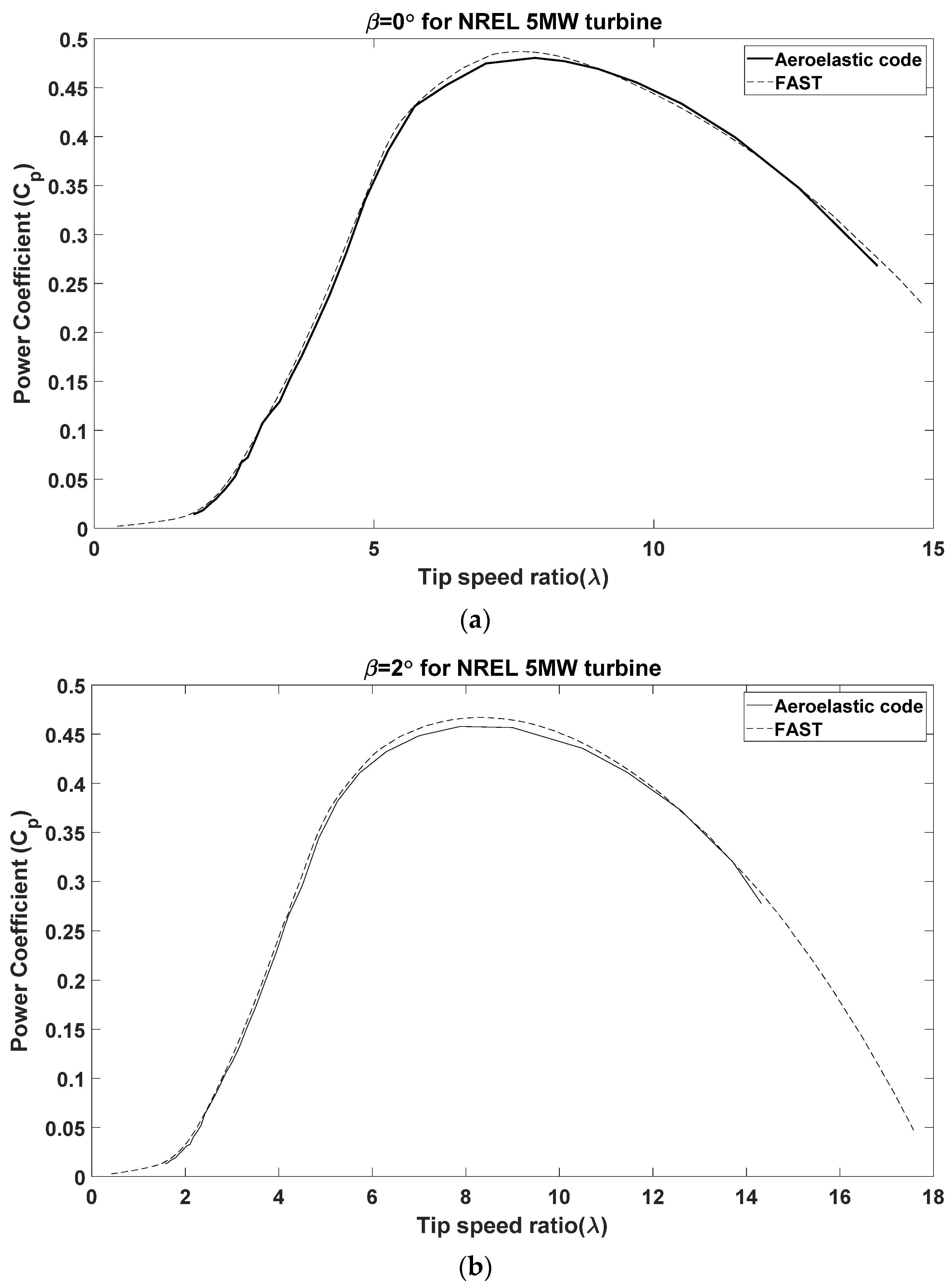
In Figure 8, the power coefficient is given as a function of tip speed ratio at different pitch angles (in degrees), and the results are compared with the FAST code. As can be seen, the results are compatible with the FAST simulations.

Remark 5.

The source FAST code is compiled with the SIMULINK/MATLAB and it is possible to validate the performance of the control algorithm on the open loop model of the wind turbine and there is a module for designing the tuned mass damper. However, as far as we know, there is no place to both consider the effect of vibration absorbers and control algorithms on the power generation and dynamic loads. In addition, the aeroelastic code will be investigated in our future work for designing various types of vibration absorbers, besides tuned mass dampers.

4. Designing the Sliding Mode Approach in the Low and High Values of Wind Speed

In this section, the power control problem for low and high values of wind speed is investigated from a load mitigation perspective. According to [3], the aeroelastic interaction of the blades and tower to the drivetrain is insignificant and can be ignored for control purposes. Therefore, the simplified model of the drivetrain can be obtained as [22,28]:

$$\{\begin{array}{l}{\dot{\omega }}_r=\frac{T_a-K_{ls}\left({\theta }_r-{\theta }_{ls}\right)-D_{ls}\left({\omega }_r-{\omega }_{ls}\right)-D_r{\omega }_r}{j_r}\\ {\dot{\omega }}_{ls}=\frac{-T_e{n}_g+K_{ls}\left({\theta }_r-{\theta }_{ls}\right)+D_{ls}\left({\omega }_r-{\omega }_{ls}\right)-D_g{n}_g^2{\omega }_{ls}}{j_g{n}_g^2}\end{array}$$

(35)

where $j_r$ and $j_g$ are rotor inertia (including the blades and rotor) and generator inertia respectively. ${\omega }_r$ and ${\omega }_{ls}$ are rotor speed and low-speed shaft speed (${\omega }_{ls}=\frac{{\omega }_g}{n_g}$) respectively. All the parameters of the model for the NREL 5MW turbine can be found in [11].

Remark 6.

In Equation (35), the blade and rotor are assumed as a rigid disk. Therefore, this model does not give any sense regarding the vibration loads. For considering the vibration loads a full aeroelastic model is needed which are developed in the previous part.

4.1. Control Problem in the Low-Speed Range of Wind Velocity

In region II, the main goal is to extract as much energy as possible from the wind. As stated before, the actuator is controlled by the torque from the generator. To achieve maximum energy, the power coefficient must be at its maximum value. For the NREL 5MW turbine, the optimum tip speed ratio (${\lambda }_{opt}$) is 7 and the optimum pitch angle is 0 degrees [11]. Therefore, the optimum rotor speed (${\omega }_{opt}$) is obtained as:

$${\lambda }_{opt}=\frac{R{\omega }_{opt}}{V}\Rightarrow {\omega }_{opt}=\frac{{\lambda }_{opt}V}{R}$$

(36)

where V is the effective wind velocity (EWV). In our previous research [23], we demonstrate how to estimate EWV, also, a detailed study can be found in [51]. Now, by defining the error signal as the difference between the optimum speed and the rotor speed, the generator’s torque must be regulated in order to minimize the error signal. Next, we introduced a novel super twisting sliding mode control approach with an observer to estimate the unknown terms to achieve maximum power [52,53].

Theorem 1.

The following generator torque ($T_e$) is suitable for maximizing the power coefficient and output power.

$$\begin{array}{l}{T}_e=-v_l\frac{j_r{j}_g{n}_g^2}{D_{ls}}\\ v_l=a_L{\displaystyle {\int }_0^t{e}_{l}dt}+b_L{\dot{e}}_l+c_L{e}_l-{\ddot{\omega }}_{opt}+{\omega }_{rej,l}\\ {\omega }_{rej,l}={\lambda }_{0,l}{\left|s_l\right|}^{1/2}sign\left(s_l\right)+{\eta }_l\\ {\dot{\eta }}_L={\lambda }_{1,l}{\left|s_l\right|}^{1/2}sign\left(s_l\right)\\ where\hspace{0.17em}\{\begin{array}{l}{s}_l=\dot{e}+{\zeta }_l\\ {\dot{\zeta }}_l=-{\ddot{\omega }}_{opt}+v_l-{\omega }_{rej,l}\\ {\lambda }_{0,l}=1.5\sqrt{L_1}\\ {\lambda }_{1,l}=1.1\sqrt{L_1}\\ \left|\frac{d\Delta {\psi }_{unknown,l}}{dt}\right|<L_1\end{array}\end{array}$$

(37)

where  $T_e$ is the generator torque,  $v_l$ is the virtual controller in region II,  ${\omega }_{rej,l}$ is the rejection term in region II (to reject uncertainties and unknown variables).

Proof. 

By defining the error signal as $e_l={\omega }_r-{\omega }_{opt}$, and according to Equation (37), one can reach the following equation:

$$\begin{array}{l}{\ddot{e}}_l=\frac{{\dot{T}}_a-\left(D_{ls}+D_r\right){\dot{\omega }}_r-K_{ls}\left({\omega }_r-{\omega }_{ls}\right)}{j_r}\\ +\frac{D_{ls}}{j_r{j}_g{n}_g^2}\left(D_{ls}\left({\omega }_r-{\omega }_{ls}\right)+K_{ls}\left({\theta }_r-{\theta }_{ls}\right)\right)-\frac{D_{ls}}{j_r{j}_g{n}_g}{T}_e-{\ddot{\omega }}_{opt}\end{array}$$

(38)

The generator torque ($T_e$) must be defined such that to stabilize the error signal. For this purpose, the generator torque must satisfy the following equation:

$${\ddot{e}}_l+a_L{\displaystyle {\int }_0^t{e}_{l}dt}+b_L{\dot{e}}_l+c_L{e}_l=0$$

(39)

In Equation (39), aerodynamic torque, time derivation of the rotor speed, and low-speed shaft speed are not measurable. Therefore, these terms must be estimated. Now, by reorganizing Equation (40), we reach the following equation:

$$\begin{array}{l}{\ddot{e}}_l={\psi }_{known}+\Delta {\psi }_{unknown}-v_l\\ where\\ \Delta {\psi }_{unknown,l}=\frac{{\dot{T}}_a-\left(D_{ls}+D_r\right){\dot{\omega }}_r-K_{ls}\left({\omega }_r-{\omega }_{ls}\right)}{j_r}\\ +\frac{D_{ls}}{j_r{j}_g{n}_g^2}\left(D_{ls}\left({\omega }_r-{\omega }_{ls}\right)+K_{ls}\left({\theta }_r-{\theta }_{ls}\right)\right)\\ {\psi }_{known,L}=-{\ddot{\omega }}_{opt}\\ v_L=-\frac{D_{ls}}{j_r{j}_g{n}_g^2}{T}_e\end{array}$$

(40)

One should note that the term ${\psi }_{known,l}$ defines the known terms of ${\ddot{e}}_l$ and $\Delta {\psi }_{unknown,l}$ denotes the unknown terms, which must be estimated and $v_l$ is the virtual control signal. For designing the control signal $v_l$, we need to estimate the disturbance term $\Delta {\psi }_{unknown,l}$. For this purpose, a first-order dynamic system is introduced as follows [54]:

$$\begin{array}{l}{s}_l={\dot{e}}_l+{\xi }_l\\ {\dot{\zeta }}_l=-{\psi }_{known,l}+v_l-{\omega }_{rej,l}\end{array}$$

(41)

The Lyapunov function $V_l=\frac{1}{2}{s}_l^2$ is introduced, giving:

$${\dot{V}}_l=s_l{\dot{s}}_l=s_l\left({\ddot{e}}_l+{\dot{\xi }}_l\right)$$

(42)

The goal is to design the term ${\omega }_{rej,l}$ to reject the uncertainties. The rejection term must be designed in such a way ${\dot{V}}_l\le -\eta \left|s_l\right|$ where $\eta$ is a positive number. By a combination of Equations (42) and (49), one can reach:

$$\begin{array}{l}{\dot{V}}_l=s_l{\dot{s}}_l=s_l\left(\Delta {\psi }_{unknown,l}-{\omega }_{rej,l}\right)\le \Vert \left|s_L\right|\Vert \Vert \Delta {\psi }_{unknown,L}\Vert -s_l{\omega }_{rej,l}\le -\eta \Vert s_l\Vert \\ \Rightarrow {\omega }_{rej,l}\ge \left(\eta +L_{slide}\right)sign\left(s_l\right)\end{array}$$

(43)

where $L_{slide}$ is a positive number which $\Vert \Delta {\psi }_{unknown}\Vert \le L_{slide}$. To reach origin asymptotically, we must have:

Finally, combining Equations (46) and (50) the control signal gives the control signal $v_l$ (${\rho }_L=\left(\eta +L_{slide}\right)$):

$$v_l=a_L{\displaystyle {\int }_0^t{e}_{l}dt}+b_L{\dot{e}}_l+c_L{e}_l-{\ddot{\omega }}_{opt}+{\rho }_{L}sign(s_l)$$

(44)

where $a_L$, $b_L$ and $c_L$ are positive coefficients which can be found in Appendix C. To design the rejection term, according to [51], the super twisting control method has a better performance in chattering rejection as well as better tracking ability. Therefore, the rejection term is defined as [54]:

$$\begin{array}{l}{\omega }_{rej,l}={\lambda }_{0,L}{\left|s_l\right|}^{1/2}sign\left(s_l\right)+{\eta }_l\\ {\dot{\eta }}_l={\lambda }_{1,L}sign\left(s_l\right)\end{array}$$

(45)

In [54], a thorough discussion has been provided to select properly the parameters ${\lambda }_{0,L}$ and ${\lambda }_{1,L}$. Accordingly, two acceptable values for these two parameters are ${\lambda }_{1,L}=1.1\sqrt{L_1}$ and ${\lambda }_{0,L}=1.5\sqrt{L_1}$ where $L_1$ is the upper bound of ${\dot{\psi }}_{unknown,l}$.

Finally, by finding the virtual control signal $v_l$, the generator torque in each time step can be updated as follows:

$$T_e=-v_l\frac{j_r{j}_g{n}_g^2}{D_{ls}}$$

(46)

□

The whole structure of the designed control system is depicted in Figure 9.

Remark 7.

To obtain the value of ${\ddot{\omega }}_{opt}$, according to Equation (44), we need the second-time derivation of EWV. We used the following derivative estimation which is proposed in [54].

$$\begin{array}{l}{v}_{estimate,1}={\dot{z}}_0=-2{L_{estimate}}^{\raisebox{1ex}{$1$}\!\left/ \!\raisebox{-1ex}{$3$}\right.}{\left|z_0-V\left(t\right)\right|}^{\raisebox{1ex}{$2$}\!\left/ \!\raisebox{-1ex}{$3$}\right.}sign\left(z_0-V\left(t\right)\right)+z_0\\ v_{estimate,2}={\dot{z}}_1=-1.5{L_{estimate}}^{\raisebox{1ex}{$1$}\!\left/ \!\raisebox{-1ex}{$2$}\right.}{\left|z_1-v_{estimate,1}\right|}^{\raisebox{1ex}{$1$}\!\left/ \!\raisebox{-1ex}{$2$}\right.}sign\left(z_1-v_{estimate,1}\right)+z_1\\ {\dot{z}}_2=-1.1L_{estimate}sign\left(z_0-v_{estimate,2}\right)\end{array}$$

(47)

where $z_0$is the estimation of $V\left(t\right)$, $z_1$is the estimation of $\dot{V}\left(t\right)$, and $z_2$is the estimation of $\ddot{V}\left(t\right)$. $L_{estimate}$is a positive number which must satisfy $\stackrel{⃛}{V}\left(t\right)\le L_{estimate}$. In this research, we assumed $L_{estimate}$= 10. More details can be found in [54].

4.2. Control Problem Inregion III

The output power must be limited to the nominal power in region III to prevent any damage to the wind turbine due to high winds. For this purpose, the rotor speed must be compared to the reference rotor speed, which is 12.1 rpm for NREL 5MW. The difference between the rotor speed and the nominal value (12.1 rpm) can be communicated via an error signal in each time step. The pitch angle actuator system usually acts as a linear servo system. According to [9,24,55], the dynamic equation of the pitch system can be described as follows:

$$\dot{\beta }=-\frac{1}{\tau }\left(\beta -u\right)$$

(48)

where $u$ is the input signal in region III. $\beta$ is the 11th DOF in the fully coupled model of NREL 5MW. For the NREL 5MW wind turbine, the pitch angle dynamic can be changed in the range of 0 and 90 degrees ($\beta \in \left[0,90\right]$), and the pitch rate cannot exceed 10 degrees per second ($\left|\dot{\beta }\right|<10\raisebox{1ex}{$\mathrm{deg}$}\!\left/ \!\raisebox{-1ex}{$s$}\right.$) [11,56]. In the following, the pitch angle mechanism is described for limiting the output power without measuring the aerodynamic torque.

Theorem 2.

The following pitch regulator signal (u) can regulate the output power to its nominal value.

$$\begin{array}{l}u=-\frac{\tau v_h{j}_r}{\frac{\partial T_a}{\partial \beta }}\\ v_h=a_h{\displaystyle {\int }_0^{t}edt+}{b}_h\dot{e}+c_{h}e-\frac{\partial T_a}{\partial \beta }\frac{\beta }{\tau j_r}+{\omega }_{rej,h}\\ {\omega }_{rej,h}={\lambda }_{0,h}{\left|s_h\right|}^{1/2}sign\left(s_h\right)+{\eta }_h\\ {\dot{\eta }}_h={\lambda }_{1,h}sign\left(s_h\right)\\ where\hspace{0.17em}\{\begin{array}{l}{s}_h={\dot{e}}_h+{\zeta }_h\\ {\dot{\zeta }}_h=-\frac{\frac{\partial T_a}{\partial \beta }\beta }{\tau j_r}+v_h-{\omega }_{rej,h}\\ {\lambda }_{0,h}=1.5\sqrt{L_2}\\ {\lambda }_{1,h}=1.1L_2\\ \left|\frac{d\Delta {\psi }_{unknown,h}}{dt}\right|<L_2\end{array}\end{array}$$

(49)

where u is the control signal,  $v_h$ is the virtual controller, $\beta$ is the pitch angle, ${\omega }_{rej,h}$ is the rejection term in region III (to reject uncertainties and unknown variables), and $\frac{\partial T_a}{\partial \beta }$ is the pitch sensitivity.

Proof. 

By defining the error signal as $e_h={\omega }_r-12.1$, and according to Equation (35), the second derivative of the error signal can be computed as follows (We simplified ${\dot{T}}_a$ by the simple chain derivation rule, ${\dot{T}}_a\left(V,{\omega }_r,\beta \right)=\frac{\partial T_a}{\partial {\omega }_r}{\dot{\omega }}_r+\frac{\partial T_a}{\partial V}\dot{V}+\frac{\partial T_a}{\partial \beta }\dot{\beta }$):

$${\ddot{e}}_h=\frac{\frac{\partial T_a}{\partial {\omega }_r}{\dot{\omega }}_r+\frac{\partial T_a}{\partial V}\dot{V}-\frac{\partial T_a}{\partial \beta }\frac{\beta }{\tau }-\left(D_{ls}+D_r\right){\dot{\omega }}_r-K_{ls}\left({\omega }_r-{\omega }_{ls}\right)+D_{ls}{\dot{\omega }}_{ls}}{j_r}+\frac{\partial T_a}{\partial \beta }\frac{u}{\tau j_r}$$

(50)

Just like the previous part, the pitch angle actuator must stabilize the rotor speed error. Therefore, the following equation must be satisfied [37]:

$${\ddot{e}}_h+a_h{\displaystyle {\int }_0^t{e}_{h}dt}+b_h{\dot{e}}_h+c_h{e}_h=0$$

(51)

where, $a_h$, $b_h$, and $c_h$ are some positive numbers. In addition, the time derivative of rotor speed, low-speed shaft speed, and wind velocity are unknown and must be estimated. To estimate the uncertainties, after simple calculations, the following equations are obtained:

$$\begin{array}{l}{\ddot{e}}_h={\psi }_{known,h}+\Delta {\psi }_{unknown,h}-v_h\\ where\\ \Delta {\psi }_{unknown,h}=\frac{\frac{\partial T_a}{\partial {\omega }_r}{\dot{\omega }}_r+\frac{\partial T_a}{\partial V}\dot{V}-\left(D_{ls}+D_r\right){\dot{\omega }}_r-K_{ls}\left({\omega }_r-{\omega }_{ls}\right)+D_{ls}{\dot{\omega }}_{ls}}{j_r}\\ {\psi }_{known}=-\frac{\partial T_a}{\partial \beta }\frac{\beta }{\tau j_r}\\ v_h=\frac{\partial T_a}{\partial \beta }\frac{u}{\tau j_r}\end{array}$$

(52)

The term $\Delta {\psi }_{unknown,h}$ is unknown and must be estimated and $v_h$ is the virtual controller in region III. For this purpose, the sliding mode approach is used similarly to the previous part. At the first, the sliding manifold is chosen as follows:

$$\begin{array}{l}{s}_h={\dot{e}}_h+{\xi }_h\\ {\dot{\zeta }}_h=-{\psi }_{known,h}+v_h-{\omega }_{rej,h}\end{array}$$

(53)

By considering the Lyapunov function as $V_h=\frac{1}{2}{s}_h^2$ and doing the same process as the previous part:

$$v_h=a_h{\displaystyle {\int }_0^{t}edt+}{b}_h\dot{e}+c_{h}e-\frac{\partial T_a}{\partial \beta }\frac{\beta }{\tau j_r}+{\rho }_{h}sign(s_h)$$

(54)

Finally, by finding the virtual control signal $v_h$, the pitch controller can be obtained as follows:

$$u=-\frac{\tau v_h{j}_r}{\frac{\partial T_a}{\partial \beta }}$$

(55)

□

As stated before, the objective of this part is to design a novel sensorless controller in region III to both control the output power and reduce the vibration loads. According to Equation (55), $\frac{\partial T_a}{\partial \beta }$ is still unknown and must be estimated. The term $\frac{\partial T_a}{\partial \beta }$ is called pitch sensitivity and indicates how the aerodynamic torque or the aerodynamic power varies with pitch angle. Pitch sensitivity depends on EWV, pitch angle, and rotor speed. In this research, pitch sensitivity is estimated by using ANFIS (Adaptive Neuro-Fuzzy Inference System), which is a fuzzy inference system that is implanted into the neural network frame [57]. Fuzzy inference systems can be categorized into the Mamdani and Takagi-Sugeno (TS) systems [57]. The difference between these systems is the output of each If-Then fuzzy rule. In the TS fuzzy system, the output of each rule is a linear combination of the inputs, but in the regular Mamdani fuzzy system, each output is a linguistic variable that is described by membership functions. Pitch sensitivity depends on the rotor speed, pitch angle, and EWV. The training data for the estimation process is obtained by FAST. The grid partition method is used for generating the FIS (fuzzy inference system) and for training the ANFIS system, the hybrid method is considered. 70% of the extracted data is used for training and the other 30% is for testing the generated model (The details of extracting data can be found in [11]). For two inputs (EWV and pitch angle) five Gaussian membership functions are considered and for the third input (rotor speed) three membership functions are considered, therefore, for the whole system, 75 rules are required. Figure 10 shows the ANFIS surface as a function of pitch angle and effective wind velocity.

Figure 11 shows the pitch sensitivity at different mean wind velocities and a constant turbulent intensity of 10%. In order to consider the effect of turbulence on the estimation process, pitch sensitivity is investigated at a constant mean wind velocity of 20 m/s and different turbulence intensities (Figure 12). As can be observed, the proposed method has an excellent performance in the estimation of pitch sensitivity. The whole structure of the control system is shown in Figure 13.

The control parameters can be found in Appendix C.

5. Load Mitigation of the Tower Vibration Loads by Using TMD

In this section, the load mitigation of the tower of the NREL 5MW has been considered by using a vibration absorber. According to [32,34], load mitigation was considered at a constant rotor speed and ignoring the drivetrain system of a wind turbine. According to [58], the standard deviation of the pitch angle can significantly affect the vibration loads of the tower. The wind turbine’s tower can be modelled as a beam that is fixed at the bottom with a concentrated mass (the nacelle) attached to the free end. This structure has two main sources of excitation:

• The vibration loads are transmitted from the blades to the hub and finally to the tower. These vibration loads can be influenced by the drivetrain control algorithms in the previous section.
• Aerodynamic loads from the wind.

According to [58], the aerodynamic loads of the tower are negligible in comparison to the first source of excitation; in other words, designing the vibration absorbers without considering the control algorithms would result in inaccuracies. To consider the effect of coupling between the drivetrain dynamic and the turbine on the load analysis, in Figure 14, the change between STD of nacelle fore-aft displacement and the two cases are considered in region III. The first case is the fully coupled model which is described in this research and is validated by FAST. The second case is the uncoupled model with constant rotor speed (12.1 rpm) and without considering the effect of the drivetrain and the pitch actuator. For this purpose, we defined the following parameter:

$${\gamma }_{difference}=\frac{{\sigma }_{couple}-{\sigma }_{uncouple}}{{\sigma }_{couple}}\times 100$$

(56)

where ${\sigma }_{couple}$ is the STD of the parameter (nacelle fore-aft displacement and flapwise displacement of the blade) in the coupled model, ${\sigma }_{uncouple}$ is the STD of the parameter in the uncoupled model, and ${\gamma }_{difference}$ denotes the difference between the coupled and uncoupled model. As can be seen, the difference is significant and any load analysis and load mitigation perspective must consider the coupled model.

In this section, by considering the control algorithm in the previous section, a TMD system is designed to reduce the fore-aft vibration of the tower. In order to design the absorber, another DOF must be considered in the aeroelastic model.

$$\left\{q_{absorber}\right\}=\left\{q_{fa,abs}\right\}$$

(57)

Also, the kinetic energy, potential energy, and external work related to the damper of the absorber system can be calculated as [30]:

$$\begin{array}{l}{T}_{absorber}=\frac{1}{2}{m}_{fa,abs}{\dot{q}}_{fa,abs}^2\\ {\pi }_{absorber}=\frac{1}{2}{k}_{fa,abs}{\left(q_{fa,abs}-q_{fa}\right)}^2\\ \delta W_{absorber}=-c_{fa,abs}\left(q_{fa,abs}-q_{fa}\right)\left(\delta q_{fa,abs}-\delta q_{fa}\right)\end{array}$$

(58)

where $m_{fa,abs}$, $k_{fa,abs}$ and $c_{fa,abs}$ are the mass, stiffness, and damping coefficient of the TMD in the fore-aft direction and $T_{absorber}$, ${\pi }_{absorber}$, and $\delta W_{absorber}$ are the kinetic energy, potential energy, and the virtual work of the damper respectively. The main goal is to design the parameters $\left\{m_{fa,abs},k_{fa,abs},c_{fa,abs}\right\}$ to minimize the fore-aft vibration signal.

Remark 8.

In Section 2 and Section 3, we defined an 11 DOFs model. In this section, other DOFs (related to the TMD) must be considered. In other words, the new size of the matrices M and N in Equation (38) are 11 × 11 and the size of vector K is 11 × 1.

6. Simulation Results

In this section, a complete aeroelastic simulation has been done by considering the control signal and the tuned mass damper in the nacelle of the wind turbine. These simulations considered 12 DOFs (6 DOFs for the blade, 2DOFs for the tower, 2DOFs for the drivetrain, 1 DOF for the pitch actuator, and 1 DOF for the absorber) of the wind turbine dynamic system. The simulation was run on MATLAB to investigate two load cases in region II and region III. The load case in region II was with a mean wind speed of 8 m/s and turbulence intensity of 10%, and the other load case in region III was with a mean wind speed of 20 m/s and turbulence intensity of 10%. The performance of the designed controllers in both regions was compared with conventional controllers (ISC control algorithm in region II and the GPI controller in region III) in terms of load mitigation. The following assumptions have been considered in the aeroelastic simulations:

• The optimum rotor speed in region II is smoothed by a low pass filter with a time constant = 1 s.
• The simulation time is considered as 10 min (according to the IEC standard [33]).
• In order to prevent chattering in the super twisting sliding mode approach, the rejection term is smoothed by a low pass filter with a time constant of 1 s.

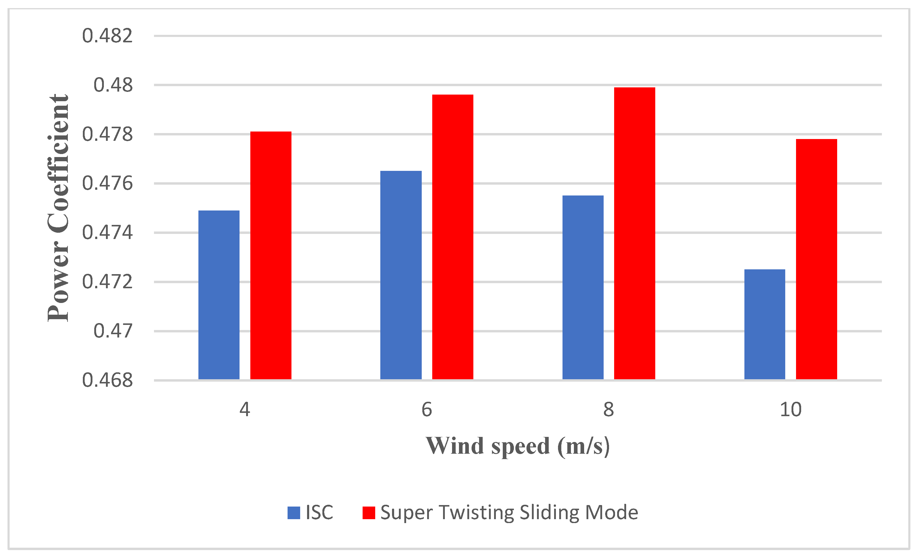
In Figure 15, the performance of the super twisting control approach was compared with the ISC algorithm in absorbing wind energy, and also the vibration loads in region II. As Figure 15 shows, super twisting sliding mode control had a better performance in increasing power coefficient in region II. However, the performance of both approaches is very similar in the terms of vibration loads. More details of the simulation can be found in

Table 3. Detailed simulation with mean wind speed 8 m/s and turbulence intensity 10%.

Control Approach	Edgewise (m)		Flapwise (m)		Output Power (kw)		Generator Torque (KN·m)
	STD	Mean	STD	Mean	STD	Mean	STD	Mean
Super twisting sliding mode	0.3452	−0.3123	0.4823	2.958	368.3	1857	2.765	20.84
MPPT algorithm	0.3457	−0.3159	0.4369	3.023	320.06	1838	2.535	20.05

.

In Figure 16, the performance of these control approaches is compared in absorbing energy from the wind. As can be seen, the super twisting control approach can improve the absorbed energy in comparison to the conventional ISC algorithm by nearly 1%.

Remark 9.

As sketched in Figure 15, the generated power of our novel approach in some regions is higher than the conventional MPPT method and in other regions, the MPPT approach generates more power. In order to have a justifiable comparison, in Figure 16 we compare the average value of the power coefficient. The averaged power coefficient has been calculated as follows:

$${\overline{C}}_p=\frac{1}{T}{\displaystyle \underset{0}{\overset{T}{\int }}{C}_{p}dt}$$

(59)

where $C_p$is the power coefficient as a function of time, T is the simulation time, which is 10 min in our work.

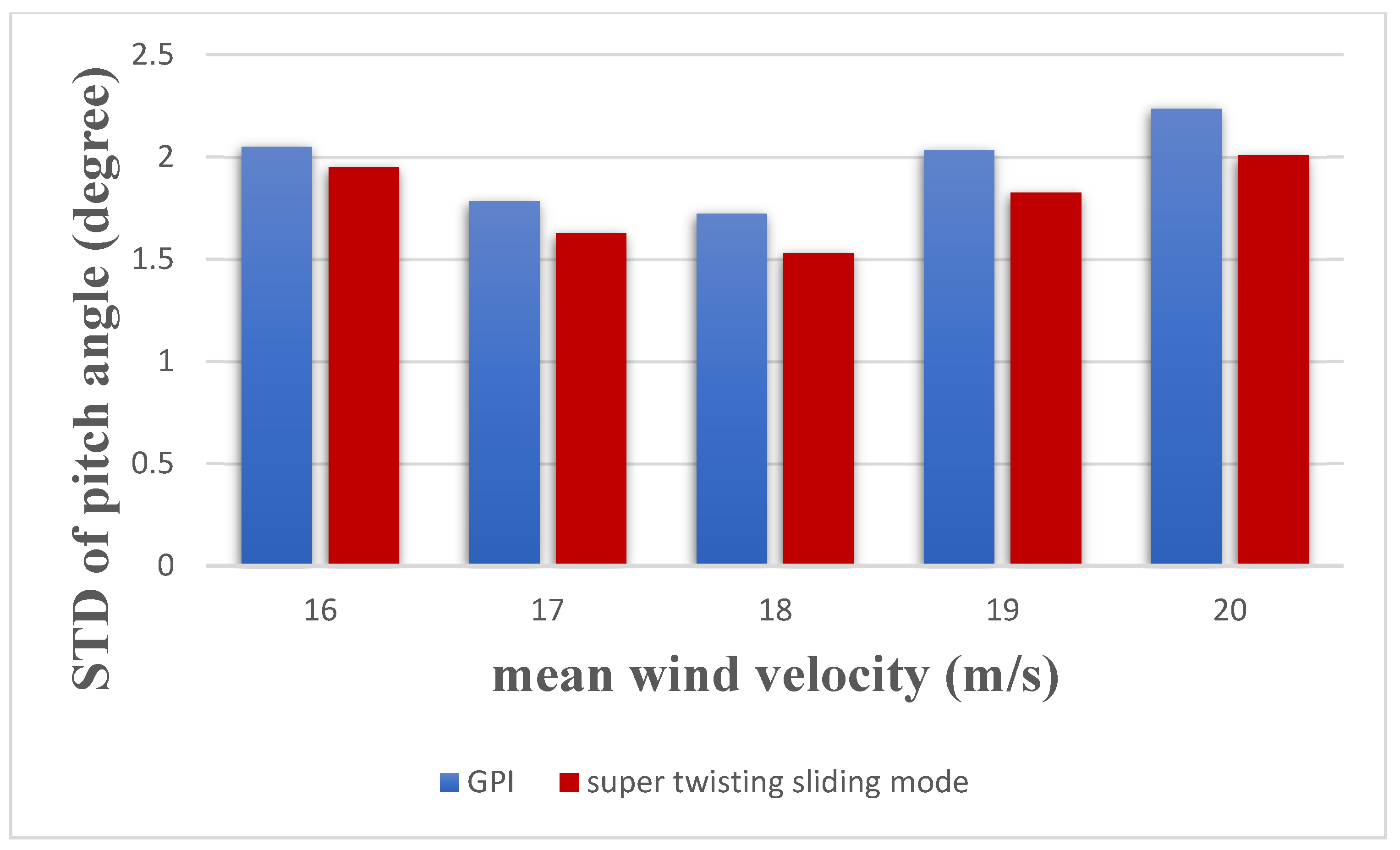
In Figure 17, the performance of the designed control system is compared with the GPI control system in region III. In

Table 4. Detailed simulation with mean wind speed = 20 m/s and turbulence intensity = 10%.

Control Approach	Edgewise (m)		Flapwise (m)		Output Power (MW)		Pitch Angle (Degree)
	STD	Mean	STD	Mean	STD	Mean	STD	Mean
Super twisting sliding mode	0.3499	−0.07541	1.048	1.413	0.1382	5.294	2.007	17.63
GPI algorithm	0.355	−0.07803	1.062	1.612	0.1503	5.31	2.236	17.18

, a complete comparison is investigated. As can be seen, the super twisting control approach has a very good ability to reduce the vibration loads of the blade in the flapwise and edgewise directions. In addition, according to Table 4, the super twisting approach has a better ability in tracking the nominal power and reducing vibration loads.

In order to consider the performance of the super twisting sliding mode control, in Figure 18, the STD of pitch angle has been investigated. As can be seen, the proposed method can reduce the STD of pitch angle by approximately 12%. In Figure 19, the reduction in the mean value of flapwise vibration has been considered. As can be seen, the super twisting sliding mode can reduce the flapwise mean value by 7% to 12% in different mean wind velocities.

For designing the TMD in the nacelle, the genetic algorithm was used for optimization with the root mean square (RMS) of the fore-aft vibration of the tower as the fitness function. For this purpose, the MATLAB optimization toolbox was used. One should note that the mass of the damper must not exceed 4% of the total mass of the rotor and nacelle [32]. Also, the stroke of the TMD in the nacelle is 8 m (because the length of the nacelle is 18 m. The best and mean individuals of the optimization process have been depicted in Figure 20. As is observed, the algorithm converges after 14 generations. The optimal results are:

$$m_{fa,abs}=12060 \mathrm{kg}, k_{fa,abs}=54070 \mathrm{N}/\mathrm{m}, c_{fa,abs}=8995 \mathrm{N}·\mathrm{s}/\mathrm{m}$$

(60)

The TMD strokes and fore-aft vibration signals are shown in Figure 21. The load reduction of the fore-aft vibration of the tower is given in

Table 5. The reduction rate of fore-aft vibration in constant mean wind speed of 20 m/s and different turbulence intensities.

Turbulence Intensity (%)	Tower Fore-Aft Reduction (%)
5	51.65
10	45.65
15	32.73
20	37.21

at different mean wind speeds with a constant turbulence intensity of 10%. The fore-aft vibration reduction of the tower at different turbulence intensities with a constant mean wind speed of 20 m/s has been investigated as seen in

Table 6. The reduction of fore-aft vibration in constant turbulence intensity of 10%, and different mean wind speed values.

Mean Wind Velocity (m/s)	Tower Fore-Aft Reduction (%)
6	40.00
8	58.46
18	33.49
20	45.65
22	35.44
24	38.27

. The load reduction is defined as follows:

$${\eta }_{red}=\frac{{\sigma }_{WTMD}-{\sigma }_{TMD}}{{\sigma }_{WTMD}}\times 100$$

(61)

where ${\eta }_{red}$ is the reduction rate, ${\sigma }_{WTMD}$ is the STD of the tower fore-aft vibration without the TMD, and ${\sigma }_{TMD}$ is the STD of the vibration signal by considering the TMD effect.

Remark 10.

The main novelty of the TMD design procedure is considering the coupled dynamics of the wind turbine. Although it must be noted that the coupled model is completely available in the FAST and other similar aeroelastic codes. However, the accuracy of the constant speed model is the main concern of this part. As demonstrated in Figure 14, the coupled dynamics of the turbine and the drivetrain makes much better accuracy in the estimation of the dynamic loads. For doing this, we compare the standard deviation of the coupled model and the uncoupled model in comparison to the blades and the tower vibration. The difference between the coupled and uncoupled models in the estimation of the dynamic loads has been discussed in Figure 14.

7. Conclusions

In this study, the wind turbine control problem has been investigated from the load reduction perspective. First, an aeroelastic model of the wind turbine was developed to consider the edgewise and flapwise vibration of the blade and also the fore-aft and side-side vibration of the tower. The blades were considered rotational beams and the tower is considered a beam with one fixed end and the other attached to a lumped mass. The Euler-Bernoulli beam theory was used to derive the dynamic behaviour of the blades and the tower. Based on the full-aeroelastic model, a reduced-order model was considered for control purposes. The control problem was investigated for both low and high wind velocities by the super twisting sliding mode control approach. In region III (high wind velocities), an adaptive neural fuzzy inference system (ANFIS) was used for estimating pitch sensitivity. The inputs of this system were pitch angle, effective wind velocity, and rotor speed. The training and test data were obtained by FAST aeroelastic code. Finally, to reduce the vibration loads of the tower, a TMD was used in the nacelle of the wind turbine to reduce the fore-aft vibration of the tower. The parameters of the TMD were chosen optimally by using the genetic algorithm. The results were compared to the baseline controllers in both operational regions which means the performance of the wind turbine system has been improved. Some findings about this research and future works are presented as follows:

• The simulation results demonstrate that the novel super twisting sliding mode approach proposed in this study can increase the power coefficient by approximately 1% (Figure 16) with no need to know state variables and aerodynamic torque (which is not measurable). In comparison with some recently published works [59,60], this work renders the stability proof of the proposed method.
• In region III, the power and rotor speed fluctuation is much smoother in comparison to the GPI control approach. This proposed method can reduce the STD of the pitch angle by 10% (Figure 19). Also, according to Figure 19, it can reduce the mean value of the flapwise vibration by 7–12% for different mean wind velocities.
• In comparison to the literature [31,32,34,35], we demonstrate that it is more accurate to consider the fully coupled model to estimate vibration loads and design vibration absorbers. In most of the previous works, the rotor speed is considered as a constant value (12.1 rpm) in region III and the drivetrain dynamic is ignored. In Figure 14, we compared the load estimation of the fully coupled model (by considering the drivetrain dynamic) and the uncoupled model (without drivetrain dynamic and constant rotor speed). As can be seen, the difference is significant in the wide range of wind velocity in region III (Figure 14).
• The TMD parameters are designed at the mean wind speed of 20 m/s in region III. Therefore, the results may be improved by considering a semi-active vibration absorber, which is optimal in both regions II and III.

References

1. Dorrell, J.; Lee, K. The cost of wind: Negative economic effects of global wind energy development. Energies 2020, 13, 3667. [Google Scholar] [CrossRef]
2. Wiser, R.; Millstein, D. Evaluating the economic return to public wind energy research and development in the United States. Appl. Energy 2020, 261, 114449. [Google Scholar] [CrossRef]
3. Bianchi, F.D.; De Battista, H.; Mantz, R.J. Wind Turbine Control Systems: Principles, Modelling and Gain Scheduling Design; Springer Science & Business Media: London, UK, 2006. [Google Scholar]
4. Boukhezzar, B.; Lupu, L.; Siguerdidjane, H.; Hand, M. Multivariable control strategy for variable speed, variable pitch wind turbines. Renew. Energy 2007, 32, 1273–1287. [Google Scholar] [CrossRef]
5. Boukhezzar, B.; Siguerdidjane, H. Nonlinear control of a variable-speed wind turbine using a two-mass model. IEEE Trans. Energy Convers. 2010, 26, 149–162. [Google Scholar] [CrossRef]
6. Boukhezzar, B.; Siguerdidjane, H. Comparison between linear and nonlinear control strategies for variable speed wind turbines. Control Eng. Pract. 2010, 18, 1357–1368. [Google Scholar] [CrossRef]
7. Errami, Y.; Benchagra, M.; Hilal, M.; Maaroufi, M.; Ouassaid, M. Control strategy for PMSG wind farm based on MPPT and direct power control. In Proceedings of the 2012 International Conference on Multimedia Computing and Systems, Tangiers, Morocco, 10–12 May 2012. [Google Scholar]
8. Han, K.; Chen, G. A novel control strategy of wind turbine MPPT implementation for direct-drive PMSG wind generation imitation platform. In Proceedings of the 2009 IEEE 6th International Power Electronics and Motion Control Conference, Wuhan, China, 17–20 May 2009. [Google Scholar]
9. Pan, C.-T.; Juan, Y.-L. A novel sensorless MPPT controller for a high-efficiency microscale wind power generation system. IEEE Trans. Energy Convers. 2009, 25, 207–216. [Google Scholar]
10. Lin, W.-M.; Hong, C.-M.; Chen, C.-H. Neural-network-based MPPT control of a stand-alone hybrid power generation system. IEEE Trans. Power Electron. 2011, 26, 3571–3581. [Google Scholar] [CrossRef]
11. Jonkman, J.; Butterfield, S.; Musial, W.; Scott, G. Definition of a 5-MW Reference Wind Turbine for Offshore System Development; National Renewable Energy Lab (NREL): Golden, CO, USA, 2009.
12. Laima, S.; Li, H.; Chen, W.; Li, F. Investigation and control of vortex-induced vibration of twin box girders. J. Fluids Struct. 2013, 39, 205–221. [Google Scholar] [CrossRef]
13. Chen, W.L.; Zhang, Q.Q.; Li, H.; Hu, H. An experimental investigation on vortex induced vibration of a flexible inclined cable under a shear flow. J. Fluids Struct. 2015, 54, 297–311. [Google Scholar] [CrossRef]
14. Chen, W.L.; Xin, D.B.; Xu, F.; Li, H.; Ou, J.P.; Hu, H. Suppression of vortex-induced vibration of a circular cylinder using suction-based flow control. J. Fluids Struct. 2013, 42, 25–39. [Google Scholar] [CrossRef]
15. Jin, X.; Cheng, P.; Chen, W.L.; Li, H. Prediction model of velocity field around circular cylinder over various Reynolds numbers by fusion convolutional neural networks based on pressure on the cylinder. Phys. Fluids 2018, 30, 047105. [Google Scholar] [CrossRef]
16. Zhang, Q.; Xiang, X.; Hui, L.; Xiong, G.; Fisher, T.S. Mechanically robust honeycomb graphene aerogel multifunctional polymer composites. Carbon 2015, 93, 659–670. [Google Scholar] [CrossRef]
17. Pan, L.; Wang, X. Variable pitch control on direct-driven PMSG for offshore wind turbine using Repetitive-TS fuzzy PID control. Renew. Energy 2020, 159, 221–237. [Google Scholar] [CrossRef]
18. Dida, A.; Merahi, F.; Mekhilef, S. New grid synchronization and power control scheme of doubly-fed induction generator based wind turbine system using fuzzy logic control. Comput. Electr. Eng. 2020, 84, 106647. [Google Scholar] [CrossRef]
19. Zadeh, L.A.; Klir, G.J.; Yuan, B. Fuzzy Sets, Fuzzy Logic, and Fuzzy Systems: Selected Papers; World Scientific: Singapore, 1996. [Google Scholar]
20. Araghi, A.R.; Riahy, G.; Carlson, O.; Gros, S. Enhancing the net energy of wind turbine using wind prediction and economic NMPC with high-accuracy nonlinear WT models. Renew. Energy 2020, 151, 750–763. [Google Scholar] [CrossRef]
21. El-Baklish, S.K.; El-Badawy, A.A.; Frison, G.; Diehl, M. Nonlinear model predictive pitch control of aero-elastic wind turbine blades. Renew. Energy 2020, 161, 777–791. [Google Scholar] [CrossRef]
22. Golnary, F.; Moradi, H. Design and comparison of quasi continuous sliding mode control with feedback linearization for a large scale wind turbine with wind speed estimation. Renew. Energy 2018, 127, 495–508. [Google Scholar] [CrossRef]
23. Golnary, F.; Moradi, H. Dynamic modelling and design of various robust sliding mode controls for the wind turbine with estimation of wind speed. Appl. Math. Model. 2019, 65, 566–585. [Google Scholar] [CrossRef]
24. Ren, Y.; Li, L.; Brindley, J.; Jiang, L. Nonlinear PI control for variable pitch wind turbine. Control Eng. Pract. 2016, 50, 84–94. [Google Scholar] [CrossRef] [Green Version]
25. Garcia, C.E.; Prett, D.M.; Morari, M. Model predictive control: Theory and practice—A survey. Automatica 1989, 25, 335–348. [Google Scholar] [CrossRef]
26. Altan, A.; Hacıoğlu, R. Model predictive control of three-axis gimbal system mounted on UAV for real-time target tracking under external disturbances. Mech. Syst. Signal Process. 2020, 138, 106548. [Google Scholar] [CrossRef]
27. Huang, S.; Lin, Y.; Chinde, V.; Ma, X.; Lian, J. Simulation-based performance evaluation of model predictive control for building energy systems. Appl. Energy 2021, 281, 116027. [Google Scholar] [CrossRef]
28. Mérida, J.; Aguilar, L.T.; Dávila, J. Analysis and synthesis of sliding mode control for large scale variable speed wind turbine for power optimization. Renew. Energy 2014, 71, 715–728. [Google Scholar] [CrossRef]
29. Mérida, J.; Aguilar, L.T.; Dávila, J. Increasing Power Generation Efficiency in Horizontal Wind Turbines by Rejecting Electromechanical Uncertainties due to the Wind. IEEE Control Syst. Lett. 2021, 6, 217–222. [Google Scholar] [CrossRef]
30. Yang, J.; He, E. Coupled modeling and structural vibration control for floating offshore wind turbine. Renew. Energy 2020, 157, 678–694. [Google Scholar] [CrossRef]
31. Zhang, Z.; Li, J.; Nielsen, S.R.; Basu, B. Mitigation of edgewise vibrations in wind turbine blades by means of roller dampers. J. Sound Vib. 2014, 333, 5283–5298. [Google Scholar] [CrossRef]
32. Sun, C.; Jahangiri, V. Bi-directional vibration control of offshore wind turbines using a 3D pendulum tuned mass damper. Mech. Syst. Signal Process. 2018, 105, 338–360. [Google Scholar] [CrossRef]
33. Jalili, N. A comparative study and analysis of semi-active vibration-control systems. J. Vib. Acoust. 2002, 124, 593–605. [Google Scholar] [CrossRef]
34. Zhang, Z.; Nielsen, S.R.; Basu, B.; Li, J. Nonlinear modeling of tuned liquid dampers (TLDs) in rotating wind turbine blades for damping edgewise vibrations. J. Fluids Struct. 2015, 59, 252–269. [Google Scholar] [CrossRef]
35. Sun, C.; Jahangiri, V.; Sun, H. Performance of a 3D pendulum tuned mass damper in offshore wind turbines under multiple hazards and system variations. Smart Struct. Syst. 2019, 24, 53–65. [Google Scholar]
36. Saravanakumar, R.; Jena, D. Validation of an integral sliding mode control for optimal control of a three blade variable speed variable pitch wind turbine. Int. J. Electr. Power Energy Syst. 2015, 69, 421–429. [Google Scholar] [CrossRef]
37. Golnary, F.; Tse, K. Novel sensorless fault-tolerant pitch control of a horizontal axis wind turbine with a new hybrid approach for effective wind velocity estimation. Renew. Energy 2021, 179, 1291–1315. [Google Scholar] [CrossRef]
38. Tong, W. Wind Power Generation and Wind Turbine Design; WIT Press: Southampton, UK, 2010. [Google Scholar]
39. Fitzgerald, B.; Sarkar, S.; Staino, A. Improved reliability of wind turbine towers with active tuned mass dampers (ATMDs). J. Sound Vib. 2018, 419, 103–122. [Google Scholar] [CrossRef]
40. Sarkar, S.; Fitzgerald, B. Vibration control of spar-type floating offshore wind turbine towers using a tuned mass-damper-inerter. Struct. Control. Health Monit. 2020, 27, e2471. [Google Scholar] [CrossRef]
41. Zhang, R.; Zhao, Z.; Dai, K. Seismic response mitigation of a wind turbine tower using a tuned parallel inerter mass system. Eng. Struct. 2019, 180, 29–39. [Google Scholar] [CrossRef]
42. Hansen, M.O. Aerodynamics of Wind Turbines; Routledge: London, UK, 2015. [Google Scholar]
43. Sun, H.; Yang, H. Numerical investigation of the average wind speed of a single wind turbine and development of a novel three-dimensional multiple wind turbine wake model. Renew. Energy 2020, 147, 192–203. [Google Scholar] [CrossRef]
44. Hansen, M.O.L.; Sørensen, J.N.; Voutsinas, S.; Sørensen, N.; Madsen, H.A. State of the art in wind turbine aerodynamics and aeroelasticity. Prog. Aerosp. Sci. 2006, 42, 285–330. [Google Scholar] [CrossRef]
45. Greenwood, D.T. Advanced Dynamics; Cambridge University Press: Cambridge, UK, 2003. [Google Scholar]
46. Jazar, R.N. Advanced Dynamics: Rigid Body, Multibody, and Aerospace Applications; John Wiley & Sons: Hoboken, NJ, USA, 2011. [Google Scholar]
47. Roithmayr, C.M.; Hodges, D.H. Dynamics: Theory and Application of Kane’s Method. ASME J. Comput. Nonlinear Dyn. 2016, 11, 11–066501. [Google Scholar] [CrossRef] [Green Version]
48. Jonkman, J.M.; Buhl, M.L., Jr. FAST User’s Guide; National Renewable Energy Laboratory: Golden, CO, USA, 2005; p. 366.
49. Jonkman, J.M. Dynamics of offshore floating wind turbines—Model development and verification. Wind Energy Int. J. Prog. Appl. Wind Power Convers. Technol. 2009, 12, 459–492. [Google Scholar] [CrossRef]
50. Jonkman, B.J. TurbSim User’s Guide, Version 1.50; National Renewable Energy Lab (NREL): Golden, CO, USA, 2009.
51. Soltani, M.N.; Knudsen, T.; Svenstrup, M.; Wisniewski, R.; Brath, P.; Ortega, R.; Johnson, K. Estimation of rotor effective wind speed: A comparison. IEEE Trans. Control Syst. Technol. 2013, 21, 1155–1167. [Google Scholar] [CrossRef]
52. Ding, S.; Hou, Q.; Wang, H. Disturbance-Observer-Based Second-Order Sliding Mode Controller for Speed Control of PMSM Drives. IEEE Trans. Energy Convers. 2022, 1–10. [Google Scholar] [CrossRef]
53. Veysi, M.; Aghaei, J.; Soltanpour, M.R.; Shasadeghi, M.; Bahrani, B.; Ryan, D.J. Robust, Accurate and Fast Decentralized Power Sharing Mechanism for Isolated DC Microgrid Using Droop-Based Sliding Mode Control. IEEE Trans. Smart Grid 2022. [Google Scholar] [CrossRef]
54. Shtessel, Y.; Edwards, C.; Fridman, L.; Levant, A. Sliding Mode Control and Observation; Springer: New York, NY, USA, 2014. [Google Scholar]
55. Lan, J.; Patton, R.J.; Zhu, X. Fault-tolerant wind turbine pitch control using adaptive sliding mode estimation. Renew. Energy 2018, 116, 219–231. [Google Scholar] [CrossRef]
56. Golnary, F.; Tse, K. Simultaneous active control of tower lateral vibration and power control of wind turbine: A novel multivariable approach. Energy Rep. 2022, 8, 4233–4251. [Google Scholar] [CrossRef]
57. Jang, J.-S. ANFIS: Adaptive-Network-based fuzzy inference system. IEEE Trans. Syst. Man Cybern. 1993, 23, 665–685. [Google Scholar] [CrossRef]
58. Lin, Z.; Chen, Z.; Liu, J.; Wu, Q. Coordinated mechanical loads and power optimization of wind energy conversion systems with variable-weight model predictive control strategy. Appl. Energy 2019, 236, 307–317. [Google Scholar] [CrossRef] [Green Version]
59. Song, D.; Liu, J.; Yang, Y.; Yang, J.; Su, M.; Wang, Y.; Gui, N.; Yang, X.; Huang, L.; Joo, Y.H. Maximum wind energy extraction of large-scale wind turbines using nonlinear model predictive control via Yin-Yang grey wolf optimization algorithm. Energy 2021, 221, 119866. [Google Scholar] [CrossRef]
60. Song, D.; Yang, Y.; Zheng, S.; Deng, X.; Yang, J.; Su, M.; Tang, W.; Yang, X.; Huang, L.; Joo, Y.H. New perspectives on maximum wind energy extraction of variable-speed wind turbines using previewed wind speeds. Energy Convers. Manag. 2020, 206, 112496. [Google Scholar] [CrossRef]
61. Moriarty, P.J.; Hansen, A.C. AeroDyn Theory Manual; National Renewable Energy Lab: Golden, CO, USA, 2005.
62. Veers, P.S. Three-Dimensional Wind Simulation; Sandia National Labs: Albuquerque, NM, USA, 1988.
Figure 1. Different operational regions of a horizontal axis wind turbine [3].
Mathematics 10 02735 g001
Figure 2. Schematic view of the drivetrain system.
Mathematics 10 02735 g002
Figure 3. Schematic view of blade and tower. (a) front view of the wind turbine. (b) side view of the wind turbine.
Mathematics 10 02735 g003aMathematics 10 02735 g003b
Figure 4. Lift, drag, thrust, and rotational forces produced by the wind interaction.
Mathematics 10 02735 g004
Figure 5. Wind speed at the hub height of the turbine.
Mathematics 10 02735 g005
Figure 6. Wind speed at two different points in the grid with a distance of 10 m (blue and red are respectively the wind velocity at left and right points with the distance of 10 m).
Mathematics 10 02735 g006
Figure 7. Schematic view of a very small component of the blade and two components of the gravity force.
Mathematics 10 02735 g007
Figure 8. Power coefficient of the NREL 5MW wind turbine as a function of tip speed ratio in three different pitch angles. A comparison between the aeroelastic code and FAST (a) β = 0 . (b) β = 2 . (c) β = 4 .
Mathematics 10 02735 g008aMathematics 10 02735 g008b
Figure 9. Schematic of the designed control system in region II.
Mathematics 10 02735 g009
Figure 10. ANFIS surface for the pitch sensitivity as a function of effective wind velocity and pitch angle.
Mathematics 10 02735 g010
Figure 11. Pitch sensitivity estimation in different mean wind speed values by using the ANFIS system. (a) 18 m/s. (b) 19 m/s. (c) 20 m/s.
Mathematics 10 02735 g011aMathematics 10 02735 g011b
Figure 12. Pitch sensitivity estimation in different turbulence intensity and constant mean wind speed of 20 m/s by using the ANFIS system. (a) 5%. (b) 10%. (c) 15%.
Mathematics 10 02735 g012aMathematics 10 02735 g012b
Figure 13. Schematic of the designed control system in region III.
Mathematics 10 02735 g013
Figure 14. The difference between the STD of the vibration loads of the coupled model and the uncoupled model. (a) fore-aft displacement of the nacelle (b) flapwise tip displacement of the blade.
Mathematics 10 02735 g014aMathematics 10 02735 g014b
Figure 15. A comparison between the performance of the classical MPPT control approach (ISC) and Super twisting sliding mode control. (a) Flapwise tip deflection of blade 1. (b) Output power. (c) Edgewise tip deflection of blade 1. (d) Rotor speed of both approaches and the optimal value.
Mathematics 10 02735 g015aMathematics 10 02735 g015b
Figure 16. Comparison between ISC control approach and Super twisting sliding mode control in absorbing wind energy in different mean wind speed values with turbulence intensity 10%. Blue is the power coefficient of ISC and red is the power coefficient according to the super twisting sliding mode control approach.
Mathematics 10 02735 g016
Figure 17. Comparison between the performance of the classical GPI control and Super twisting sliding mode control for (a) Rotor speed, (b) pitch angle, (c) Fdgewise blade 1 tip deflection, and (d) Edgewise tip deflection of blade 1.
Mathematics 10 02735 g017aMathematics 10 02735 g017b
Figure 18. Comparison between the STD of pitch angle signal in gain schedule control approach and super twisting sliding mode control in different mean wind speed values with turbulence intensity 10%.
Mathematics 10 02735 g018
Figure 19. Flapwise displacement mean reduction in different mean wind velocities. The super twisting sliding mode can reduce the mean value of vibration signal by 7% to 12% in different mean wind velocities and turbulence intensity 10%.
Mathematics 10 02735 g019
Figure 20. Iterations for finding optimal solutions. Best individuals and mean values are investigated.
Mathematics 10 02735 g020
Figure 21. TMD performance in reducing tower fore-aft vibration. (a) TMD stroke. (b) fore-aft vibration of the tower with and without TMD.
Mathematics 10 02735 g021aMathematics 10 02735 g021b