Article

The Binomial Distribution: Historical Origin and Evolution of Its Problem Situations

by
Jaime Israel García-García
*,
Nicolás Alonso Fernández Coronado
,
Elizabeth H. Arredondo
and
Isaac Alejandro Imilpán Rivera
Departamento de Ciencias Exactas, Universidad de Los Lagos, Osorno 5290000, Chile
*
Author to whom correspondence should be addressed.
Mathematics 2022, 10(15), 2680; https://doi.org/10.3390/math10152680
Submission received: 19 June 2022 / Revised: 19 July 2022 / Accepted: 26 July 2022 / Published: 29 July 2022
(This article belongs to the Special Issue Statistics Education: An Immediate Need in a Changing World)

Abstract

:
The increase in available probabilistic information and its usefulness for understanding the world has made it necessary to promote probabilistic literate citizens. For this, the binomial distribution is fundamental as one of the most important distributions for understanding random phenomena and effective decision making, and as a facilitator for the understanding of mathematical and probabilistic notions such as the normal distribution. However, to understand it effectively, it is necessary to consider how it has developed throughout history, that is, the components that gave it the form and meaning that we know today. To address this perspective, we identify the problem situations that gave origin to the binomial distribution, the operational and discursive practices developed to find solutions, and the conflicts that caused a leap in mathematical and probability heuristics, culminating in what is now known as the binomial distribution formula. As a result, we present five historical links to the binomial phenomenon where problem situations of increasing complexity were addressed: a case study using informal means (such as direct counting), the formalization of numerical patterns and constructs related to counting cases, specific probability calculus, the study and modeling of probability in variable or complex phenomena, and the use of the distribution formula as a tool to approaching notions such as the normal distribution. The periods and situations identified correspond to a required step in the design of binomial distribution learning from a historical epistemological perspective and when solving conflicts.

1. Introduction

The teaching and learning of probability have taken on great importance at the curricular and research levels over the past few decades as a consequence of technological progress, the large amount of information available, and its easy accessibility. For this, citizens should have the knowledge and dispositions that allow them to argue and critically interpret probabilistic information [1]. The consideration of such relevance is evidenced by recent changes in the focus of its teaching, from one based on formulas to one focused on experimentation and its complementation with theories, as well as the introduction of probabilistic ideas or concepts in early education [2,3,4]. This exposes challenges and weaknesses such as the fact that most current teachers may not be familiar with the different meanings of probability and the possible conflicts that their students may experience, having studied probability from a theoretical perspective [4,5]. The lack of consideration of historical, cognitive, and epistemological aspects of probability makes it easier for students to generate early misconceptions, for example, (1) about representativeness, believing that the probability for a sample depends on its similarity to the population distribution; (2) equiprobability bias, in which the student assumes that random events are equiprobable by nature; (3) the belief that a random event depends on a force beyond their control; (4) believing that there is complete human control over a random phenomenon; and (5) resolution errors, such as carelessness or the use of incorrect strategies [5,6,7,8]. This focus on preparing students for real-world probability scenarios is what Gal [1] calls probabilistic literacy, that is, the ability to access, use, interpret, and critically argue probabilistic information, as well as the control of problematic attitudes, in order to deal effectively with tasks and situations involving uncertainty and risk in real life, for which five pillars of knowledge are needed: analyzing big ideas, calculating probabilities, language, context, and critical questions. Under this perspective, aspects that are promoted in general education in the 21st century are also considered, such as theoretical epistemological knowledge, cognitive abilities, and attitudes, in order to apply it effectively in problem solving and society, which requires a conception of teaching based on the articulation between theory, practice, and context. This implies a greater demand on teachers to act as interpreters and critics who use probability to their advantage, modeling situations and generating predictions without falling into biases such as disregarding the variability of real-life phenomena [9,10], while also opening doors for its development from an early age to establish its role in active knowledge [11,12].
In the search for ways to promote this more meaningful learning of probability, learning the binomial distribution is essential since it enables the analysis of random phenomena and is closely related to other distributions such as Poisson and normal distribution, making it a notable research object of didactics in mathematics [13]. For example, Sánchez and Landín [14,15] propose and validate a hierarchy on their understanding of the SOLO taxonomy, identifying as necessary the precise handling of the concepts and ideas behind it, such as overcoming the idiosyncratic conception of probability, the representation of sequences, the classical approach to probability, the product rule, the binomial coefficient, and the binomial formula. Taufiq et al. [16] analyzed the learning of the binomial distribution in a secondary-level textbook and identified (1) an incomplete structure in the discussion of the binomial distribution by not addressing essential concepts such as discrete and continuous random variables or probability distribution; and (2) a lack of discussion of statistics related to the binomial distribution as well as their meaning. García-García et al. [17] addressed the development of the notion of the binomial distribution in high school students, identifying key elements for its understanding: the identification of patterns, the variability, the probability law of large numbers, and the identification of binomial behavior in contextual situations. These lines of research evidence a desire to characterize the understanding of the binomial distribution and to analyze how it is approached by different subjects and in educational resources.
Similar to the results of the research on probability, weaknesses in students and teachers regarding comprehension of the epistemic aspect of the binomial distribution, its fundamental components, and how they are related, have been identified. Alvarado and Batanero [18] analyzed the theoretical and practical understanding of engineering students after a teaching experiment and identified weaknesses in the application of the binomial distribution in specific situations and confusion about statistical concepts, such as variance and mean, which showed that they did not perceive the importance of the parameters of the binomial phenomenon to approach the normal distribution (31%) and the consideration of the mean of the binomial distribution as applicable in the prediction of phenomena only when the value of the trials it involved was sufficiently high (90%). Pilcue and Martínez [19] identified the difficulties experienced by undergraduate students in Basic Education with an emphasis on mathematics in interpreting the data involved in a binomial situation and understanding combinatorics using the factorial. Among the most worrying difficulties found were those in identifying a binomial phenomenon, a probabilistic phenomenon, and the parameters involved; making mistakes in components when calculating the value of the combinatorial; or using other formulas without proper construction or argumentation. Sánchez and Landín [20] proposed seven components of knowledge about the binomial distribution: recognition of Bernoulli trials, recognition of the binomial random variable, use of combinatorial trees and representations of the sequences of results, use of the classical definition of probability (Laplace), knowledge and handling of the product rule of probability, use of combinatorics and the product rule in a joint manner, and the proper use of the probability formula of the binomial distribution. They also identified in high school students a minimal effective use of the binomial formula and its associated parameters, a difficulty in linking the various components of the understanding of the binomial distribution, and the necessity to promote the understanding of the product rule and combinatorics in order to understand the binomial distribution formula. Consequently, we can confirm a link between the study of the didactics of probability in general and the one focused on the binomial distribution.
The above-mentioned research shares an important characteristic; it is based on the identification of essential elements or components to evaluate the level of understanding of the binomial distribution and to propose improvements, which is achieved by considering the binomial distribution in its formal form in the same way it is reflected in current students’ abilities or educational resources. However, as with any mathematical notion, the binomial distribution has developed throughout history, overcoming several conflicts and modifications relating to new ideas and solving new problems. This suggests that the historical development of the binomial distribution is an important component that needs to be addressed and that has a high potential to support teachers or educational leaders in solving learning conflicts [9], considering that part of this historical development will be reflected in students’ understanding of the binomial distribution. This aspect, as also mentioned by Batanero [4], is essential since it evidences how elements such as concepts and propositions have been articulated in different levels of mathematical and probability complexity to provide answers to a family of problem situations throughout history, associated with the reasoning of students and the conflicts they have witnessed during their learning processes. In conclusion, by addressing the epistemic aspect of the binomial distribution from an historical perspective, epistemological guidelines that articulate the weaknesses identified and how they are historically addressed could be generated, thus contributing to the early investigational state of the binomial distribution [21] and proposing a new didactic approach to its learning and the solving of epistemic conflicts. Thus, we are presented with the following questions: What situations can be attributed to the binomial distribution, and what knowledge of its historical evolution could optimize its understanding in the teaching and learning processes?
To identify the essential elements in the historical construction of the binomial distribution and thus facilitating its teaching and learning by considering the epistemological historical aspect, we identify the problem situations that gave it its origins and the objects involved in its evolution and formalization throughout history by conducting an Historical Epistemological Study (HES). As the main conclusion of our study, we identified that the binomial distribution took shape during five important periods in which the problems addressed the increase in complexity and are the result of the development of probability theory: (1) case count in ancient India and Greece, (2) the formalization of numerical patterns and mathematical constructs such as the Pascal triangle, (3) the calculation of point probabilities originated with probability theory in search of solutions to problem situations such as the problem of points, (4) the informal construction of the binomial distribution by Pascal and Fermat in search of more general solutions to probabilistic phenomena, and (5) the formalization of the binomial distribution formula by Bernoulli and its use as a modeling tool to approach other phenomena within probability theory. For the contribution of this work, we propose a proper characterization of the binomial distribution from its more informal ideas based on its uses throughout history and how these can be related to students’ work in the classroom. This has potential for the longitudinal learning of this construct within educational programs such as those in Chile [22], which propose that ideas associated with the binomial phenomenon are introduced from 6th grade in an informal way, leaving its formalization and use in decision making for the last years of high school, but without presenting a clear relationship between its components and how the formula originated from mathematical and probabilistic principles.

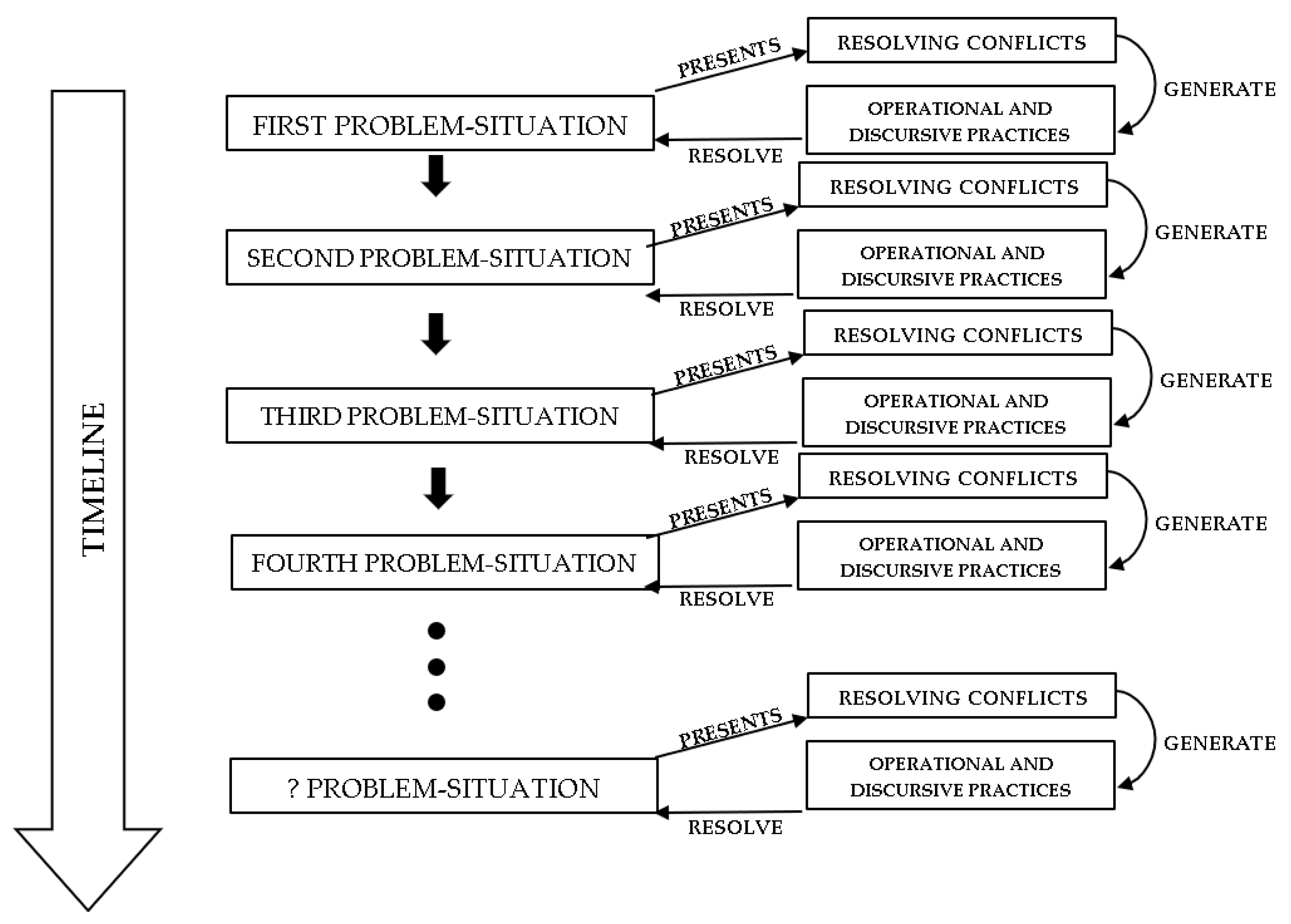
2. Theoretical Framework

For promoting probability literacy related to the binomial distribution, it can be considered that the disarticulation between the different applications of a mathematical and a probabilistic notion will be problematic for the design of its teaching in essential aspects such as problem solving and critical thinking. Batanero [5] stresses the importance of this aspect, indicating that the teaching of probability cannot be limited to a single perspective since they are all dialectically linked; thus, she invites research of a historical nature, closely related to the experimentation and historical trials and errors that can also be presented in the classroom.
For this task, we considered the realization of a Historical Epistemological Study (HES) based on the epistemic principle of the Ontosemiotic Approach to Mathematical Knowledge and Instruction (OSA) [23,24,25], used in probability research for the historical reconstruction of the meaning of the central limit theorem [26] and the chi-squared statistic [27]. This principle is also used in the development of the competencies of mathematics teachers, who not only require formal disciplinary knowledge but also competencies and skills for the adequate management of this construct for different problem situations to give it a place in relation to other mathematical and probabilistic knowledge and solve the learning conflicts of students [28]. From the OSA perspective, and to answer the epistemic question of mathematics, mathematics is considered the product of the human being, a series of practices originated to provide a solution to a problem situation, communicate that solution, validate it, and use it to address new ones [29]. These practices can be operative or discursive [30]; the first one corresponds to competence with respect to a mathematical construct, for example, in the use of arithmetic operations or models to find an answer, whereas the other is closely related to the social aspects of knowledge in terms of knowing what a mathematical construct is and what it is for, in other words, its understanding. Both are essential components of what Gal [1] referred to as probabilistic literacy and have a clear role in the idea that probability is presented as a way of modeling the world, analyzing random situations, and even seeking which of them are favorable, which is an important part of the search for human welfare. Therefore, knowledge of the binomial distribution can be evidenced in many ways depending on how people use it to approach problem situations from a simple coin toss to the study of probability density or its mean, making a historical study a potential provider of an overview of the reasoning of a student at various stages in the construction of knowledge of this object.
For addressing the epistemic aspect of mathematical objects, from an historical perspective, the HES [31] has predominantly been used [4,28,32,33]. This type of study addresses the nature, genesis, and consolidation of concepts or ideas, attributing a complexity due to the different aspects that originated and formed them throughout history, and thus, as part of the OSA’s theoretical and methodological framework, it is an effective approach to identifying the elements needed to analyze the teaching–learning process of the binomial distribution considering its historical epistemological aspect, that is, a chronological delimitation of wise knowledge [34]. Witzke et al. [35] similarly indicated that the importance of conducting this type of study lies in responding to the problem of the lack of consideration of historical elements in teaching, that is, a historical decontextualization, which has generated an important discussion about the contributions about its genesis that would help to understand its current teaching.
One of the primary examples of the use of an HES on probability learning was a study by Batanero [4] who used an HES to analyze various historical meanings that have been given to probability, for example, as a reason (favorable and unfavorable cases), as evidence of empirical reality, as a personal belief and, formally, as a mathematical model to understand the real world. Subsequently, from these elements and their articulation within the notions of OSA, she identified elements that led to the identification of the meaning of probability and in contrast, analyze the way it is presented in educational processes. Ruiz [36] presented her work based on the realization of an HES on the random variable and identifies an informal stage prior to probability itself, which was approached as probability theory developed with a focus on primitive games of chance and the study of bets. Finally, we highlight the research conducted by Lemus-Cortez and Huincahue [37] that consists of an HES on the normal distribution with the aim of analyzing and evaluating an epistemic route for a conceptual approach and generating teaching–learning processes from a multidisciplinary approach, particularly focused on the area of medicine, with the intent of promoting the articulation between theory and practice in how students of 17 and 18 years model tasks and collect data.
Based on these premises and in relation to our objective, we conclude that identifying the main problem situations that provided the origins and development of the binomial distribution, as well as the practices for its resolution, will help us to understand its comprehension by students and explore how it is presented in the curricula. Therefore, the HES could help us to address this unexplored area of mathematical and probabilistic constructs as the first step of an in-depth study with the objective of promoting the essential elements for its adequate teaching and learning.

3. Methodology

The study presented is of a qualitative type [38] since it consists of the identification and analysis of the problem situations that have given meaning to the binomial distribution throughout history. In addition, it is conducted at an exploratory-descriptive level [39] to understand the background of what is presented to us as the binomial distribution, which has not yet been studied from a historical epistemological perspective, through the analysis and organization of information that has been collected on it. For the latter, a documentary design is followed [40] in which knowledge of the binomial distribution is recovered, systematized, and analyzed from a bibliography that addresses its history.
For this first approach to identifying how the binomial distribution has developed throughout history, our work consisted of three phases, each one with a specific objective: (1) the selection and recollection of the appropriate bibliography, (2) its analysis and synthesis, and (3) the proposal of a characterization of the binomial distribution from its historical development and identified practices (operative and discursive).
The first phase consisted of the collection and analysis of the literature in which the binomial distribution is explicitly addressed and presents the problem situations and solution practices associated with the binomial phenomenon or its formula [41,42,43,44]. As our focus is on the historical perspective of the binomial distribution, we did not consider the literature in which it was presented exclusively as a finalized construct, that is, in a formal way and as an instrument for the direct analysis of situations. Likewise, some articles that addressed the binomial distribution were not considered for this analysis if they did not do so from the desired perspective; however, they were considered in order to make a contrast and highlight the potential of the HES and how it complements and is complemented by them.
The second phase consisted of the organization and analysis of the information collected, identifying the historical periods in the development of the binomial distribution, the key events that caused an increase in the heuristics of the phenomena addressed, and the operative and discursive practices involved. This was achieved using the hermeneutic method [45], which considers that the human being has a consciousness of a historical character and is full of prejudices of a theoretical and practical nature, which reflects the experiences or senses associated with knowledge. Consequently, to understand the process whereby preconceptions advanced in the search for meaning to be composed of intellect, explanation, and application, which we consider key events in the development of the binomial distribution, the resolution of problem situations required a new approach with higher heuristics.
Finally, as a result of the previous phase, a synthesis of the historical development of the binomial distribution is proposed (see Figure 1). From this, we expect to represent the sequence of its construction and the emergence of its essential elements that could help with the development of the line of research from this perspective.

4. The History of the Binomial Distribution

This historical epistemological study allowed us to identify five periods in the development of the binomial distribution, characterized by the complexities of the problem situations addressed. In the following subsections, we describe the problem situations identified, their resolutive practices, and the events that signaled a new development in the complexity and formality of the approach to binomial phenomena.

4.1. The First Approach to Binomial Phenomena: Early Combinatorics and Number Patterns from Ancient India and Greece to Dante’s Divine Comedy (600 BCE—14th Century)

In this period, the first approaches by former experts to the study of probabilistic phenomena, which can also be associated with binomial situations, were presented. This is the basis for the study of random phenomena through empirical analysis, which would give way to the generation and study of numerical patterns, essential for the development of probability theory in the future and, therefore, for the formalization of the binomial distribution.
The first challenge in the development of probability theory and the study of binomial situations was to break the deterministic scheme of things and understand how mathematics could be used to model and predict real-life phenomena [42]. This meant overcoming Aristotle’s ideology that random phenomena are unpredictable and inaccessible through investigation in an empirical study that originally had mathematical imperfections and little control of the phenomena, leading it to be a theory of axiomatic character. In the Indian subcontinent, the study of the number of cases was recorded orally and documented since the classical period of Indian history, mainly grounded in religious scriptures [46].
The earliest known record of a preliminary mention of combinatorial problems is presented in the oral compilations of the encyclopedic work called the Bhagavati Sūtra (Exposition of Explanations) (5th century BC), in which answers to several questions were given in the form of a dialogue. As an extension of these problems, punctual examples were accumulated and studied for the identification of numerical patterns in an attempt to formalize them, proposing recursive rules.
Another of the earliest bases for the development of probability is identified in Greek mathematics. Porphyry presented the question of combinatorial nature by asking how many ways can two things be selected from among n different things? [43], which was solved by the direct counting of cases and recursive reasoning for the concrete case n = 5. Associated with the combinatorial phenomenon and the study of possible cases regardless of the order, it was answered with a combinatorial consideration of cases and recursive reasoning, giving the answer as 4 + 3 + 2 + 1 = 10. In a similar way, closer to the first steps in modeling general cases in probability, this occurred when Pappus of Alexandria addressed the geometric problem of the number of intersections that could be generated with n intersecting lines (with restriction), stating the solution to be equivalent to modern expressions such as triangular figured numbers [44].
1 + 2 + 3 + 4 + 5 + + ( n 1 ) = 1 2 n ( n 1 )
Although during the Middle Ages there was no evidence of the calculation of probabilities and probability associated with the binomial distribution, mathematical constructs related to the possible number of cases were already being addressed in India around 1150 in the form of permutations and combinatory with Bhaskara, and in Hindu and Arabic mathematics from 1265 in the form of the binomial expansion and arithmetical triangle. In Dante’s Divine Comedy (1320), the first indications of probability are identified in the form of proportions [41], and around the same year (1321) Levi ben Gerson became the first person in Europe to deliver the general formula of combinatorics and permutation, demonstrating them by induction [42].
In this period, the transition from the study of random phenomena through empirical ideas such as the direct counting of cases and their representation through symbolic or common language is evident (see Table 1). From the constructivist perspective, it can be associated with how students face random ideas for the first time, relating numerical patterns with inductive reasoning to construct mathematical objects. Addressing elements of the early state of probability (see Table 2), such as the sample space, these problem situations would reach their maximum complexity in the generalization of these patterns.

4.2. Development and Formalization of Numerical Patterns for Counting Cases: From Stifel’s and Pascal’s Triangles to Probability as a Numerical Notion by Arnauld and Nicole (15th Century–16th Century)

The mathematical patterns identified in the previous period and their relationships were formalized and presented in works such as Stifel’s triangle and Pascal’s triangle (Figure 2). In the latter, figurate numbers, binomial coefficients, and combinatorics were presented and related, for example, the triangular numbers (1, 3, 6, 10, 15, 21, ...) and the tetrahedral numbers (1, 4, 10, 20, 35, 56) [44].
Based on Figure 2 and considering the generating row and column as number 0, we present some of the construction rules and properties proved by Pascal in verbal form with the recursion formulas:
4.2.1.
Row m and Column n Term (tm,n):
t m , n = t m 1 , n +   t m , n 1 ,   m , n   m , n     0 , 0
t 0 , n = t m , 0 = t 0 , 0 = 1
4.2.2.
Addition of Elements from Row m to Column n
R m , n = j = 0 n t m , j  
4.2.3.
Addition of Elements from Column n to Row m
C m , n = k = 0 m t k , n
4.2.4.
Addition of Elements of the Diagonal from the First Term of Row m to the nth Element of the Diagonal
D m , n = j = 0 n t m j , j
4.2.5.
Addition of all Elements of the Diagonal
D m = D m , m
4.2.6.
Row and Column Properties
t m , n = R m 1 , n = C m , n 1
t m , n 1 = k = 0 m 1 R k , n 1 = j = 0 n 1 C m 1 , j
4.2.7.
Property of Symmetry
t m , n = t n , m
4.2.8.
Ratio Property, Proven by Induction
t m + 1 , n 1 t m , n = n m + 1
4.2.9.
Multiplicative Form of tm,n
Based on Equation (13), it can be proved that
t m , n = m + n m + n 1 m + 1 n n 1 1 = m + n C n
4.2.10.
Relation between Pascal’s Triangle Term and Combinatorics
The reasoning used by Pascal to relate the number of combinations to the term of his arithmetic triangle is as follows: The n + 1 elements can be addressed as n plus one element (A), then n+1Ck would be the combinations without A and with A. That way, the nCk would be the combinations without A and nCk-1 would be the combinations with A, since only k-1 can be selected besides A. With that, it can be proven by induction that
R n k , k = C k , n + 1
With that, based on Equation (13), it can be proved by induction that
n + 1 C k = t n + 1 k , k
In a similar way, Pascal demonstrated the relationship between the binomial coefficients and the arithmetic triangle [42,44] allowing the Pascal triangle to be represented as in Figure 3.
a + b k = i = 1 k t k i , i a k i b i
With this, Pascal’s triangle could also be used for the study of the number of possible cases. For example, in the toss of four coins, when observing the fourth diagonal it can be observed that the number of possible results will be given by the sum of the coefficients (1 + 4 + 6 + 4 + 1 = 16) and if the order does not matter (meaning that the case HTTH is equivalent to HHTT), the number of possible results will be given by the number of terms of the diagonal 5.
Until the end of the 16th century, probability was still considered a non-numerical and purely epistemological concept, its calculation being part of algebra and framed by the concept of chance and the proportion of cases while also being addressed in a verbal style [42]. Arnauld and Nicole [47] broke this scheme in 1662 using mathematical principles to present probability as a numerical value applicable to situations beyond games of chance and established the theory of probability calculation and the application of mathematical constructs to analyze the phenomena that follow random behavior.
With the above, the pursuit of the study of probability and case counting directly with expressions constructed from numerical patterns is evident (see Table 3) and is an example of the use of triangular numbers as an answer to the Pappus problem, as previously addressed. This is associated with how students work in the classroom when modeling binomial phenomena relying on binomial coefficients, Pascal’s triangle, or tree diagrams. The construct presented can be wrongly used by teachers as the correct knowledge or as a tool to verify the relationships between these elements, leaving as secondary the comprehension of their origins and arguments behind their demonstration.
As shown in Table 4, the historical characterization of the problem situations presents a pre-developing stage in the theory of probability, setting the base for analyzing the number of cases and the probability using mathematical and graphic constructs and their relationships. This, as evidenced in the study, could be achieved by encouraging students to use their own representations, articulating them with those such as Pascal’s triangle, and the identification and understanding of their construction rules and their arithmetization.

4.3. Use of Mathematical Constructs to Model Probability Situations from the Beginnings of Probability Theory with the Problem of Points to the Incomplete Binomial Distribution by Pascal and Fermat (15th–17th Centuries)

In this period, the deductive use of constructs such as combinatorics was presented, allowing the direct calculation of the probability of concrete situations and the search for solutions to more general situations. It corresponded to a major challenge, which the student is only able to address adequately once he or she understands the usefulness of the mathematical constructs already presented and articulates them with the various practices in the meaningful study of random phenomena. At the end of this period, as probability was defined as a contextualizable value and applicable to phenomena beyond games of chance for the search for beneficial situations, this type of problem was approached as a numerical value instead of as a proportion, still without unique terminology or any recourse observations of relative frequencies.
The main problem situation in the origin of probability theory was the problem of points. It consists of two players (A and B) who decide to play a series of games until one of them has won a specific number (s). The game is stopped when A has won s1 games and B has won s2 (both less than s). They then need to divide the money fairly. Its name comes from the fact that instead of considering the number of games, its resolution is based on associating each winner with a number of points and based on this, distributing the money, as in the example shown in Figure 4.
It was initially observed around 1494 by Pacioli in the specific case of s = 6, s1 = 5, and s2 = 2 and based on the proportions, he concluded that with the minimum number of sets being s and the largest number of sets being 2s − 1, the division should be s 1 2 s 1 and s 2 2 s 1 . This proposal was criticized because of the absence of probability principles [42]. This type of reasoning continued with other authors until Cardano approached it from the number of games that each player is yet to win (a = s − s1, b = s − s2); that way, he could infer a new play where A, starting from scratch, is the winner if A wins a games before B wins b games, concluding that the division should be b(b + 1) to (a + 1). A complete solution was given by Pascal and Fermat almost a century later [41,42].
Another important topic was the use of mathematical analysis for games of chance in looking for favorable situations, modeling the conditions of a game, and identifying loaded dice and frauds. These ideas were addressed by Cardano (1663), reaching the conclusion that a six-sided die is honest when each of the faces has the same possibility of occurrence and using the multiplication rule and the multiplication principles [42].
During the 17th century, Samuel Pepys and Isaac Newton analyzed the specific situations associated with the binomial phenomenon [42,44]. These were solved by the enumeration of cases and using combinatorial principles and probability without explicit reference to the binomial distribution and included (a) the probability that in six fair die tosses, at least one six is obtained; (b) the probability that in twelve fair die tosses, at least two sixes appear; and (c) the probability that in eighteen fair die tosses, at least three sixes appear. The first two were solved by combinatorial principles, whereas the last one was not solved but denoted as a value less than the one obtained in situation (b). For situation (a), all the possibilities of throwing six dice were given by 66, whereas the number of no-six appearances was 56. Therefore, the number of favorable events will be 31031. This could also be constructed from combinatorics and the product principle of probability.
6 0 1 6 0 5 6 6 = 5 6 6 = 0.33489797668038408779169519890261
A breakthrough in the study of probability began with questions about games of chance asked by Antoine Gombaud to Blaise Pascal in 1654 and communicated to Fermat. They added to the basic principles and rules of numeration the knowledge of combinatorial theory, generating what would be known as combinatorial chance and, without using the term probability, introduced the concept of value, later known as expectation.
One of the situations studied was from 1654: if one bets on rolling a six with one die, the advantage of rolling it on four is 671 to 625, and if one bets on rolling two sixes with two dice, there is a disadvantage in 24 throws. This can be obtained from the expression
1 q n q n 1   o   q n 1 2
They also arrived at conclusions such as if in a dice game the participant bets to roll a six in eight throws, the player should receive 1 6 of the total for not making the first throw, 1 6 of the remainder for not making the second throw, and so on, thus concluding that the value of the kth throw is
1 6 1 5 6 k 1
From this period, we can identify the arithmetization of probabilistic phenomena using the constructs from the previous periods in the search for solutions to a more extensive variety of problem situations (see Table 5). For the student, the historical development suggests that it is necessary to become familiar with the mathematical constructs and the principles of probability. With this ensured, the evidence shows the modeling of various probabilistic problem situations at an arithmetic level with the direct calculation of probabilities or at an algebraic level with the handling of equations or inequalities.
As shown in Table 6, the historical characterization of the problem situations presents an early or informal stage of probability theory called the theory of chances. It is related to a higher level of analysis where basic probability principles derived from the ones related to counting cases are used, with deductive and inductive reasoning that can be considered to be of an algebraic type but with a language that is still of an arithmetic type.

4.4. The Informal Binomial Distribution, from Its First Appearance in the Works of Pascal and Fermat to Its Iterations in the Works of Huygens and Arbuthnot (17th Century–18th Century)

During this period, the generalization of expressions to model binomial situations involving some unknown variable, such as the number of trials needed or particular cases, is identified. It was no longer an attempt to model only the probability associated with a probabilistic situation but also the situation itself.
Pascal also used the arithmetic triangle to study the problem of points, in specific and then in general situations and developed the binomial distribution for p = 1 2 based on combinatorics and recursive methods and Pascal’s triangle and its associated principles to model the mentioned case as follows (see Figure 5): considering e(a,b) as the money that would correspond to A if the game stops, with A needing to win a games and B needing to win b games, in the case where the maximum number of games is three and A needs to win one and B needs to win two, if A wins the next one, A should receive the total bet (1). However, if A loses the next game since they each need to win one then they should each be entitled to half the bet 1 2 . Averaging these cases, A should receive 3 4 of the total bet [42], which could also be considered as A’s probability of winning.
This formulation can be described by the following expressions relatable to a differential equation:
e 0 , n = 1
e n , 0 = 0
e n , n = 1 2
e a , b = 1 2 e a 1 , b +   e a , b 1
With this, for example, for the case s = 4, to obtain e(3,1), a recursive formula can be used:
e 3 , 1 = 1 2 e 2 , 1 +   e 3 , 0 = 1 2 1 4 + 0 = 1 8
Finally, Pascal identified that the values obtained are related to the terms in the arithmetic triangle. By induction, using as the first case a + b = 2, he demonstrated that
e a , b = D a + b 1 , b D a + b 1
That way, as an example, e(3,1) corresponds to D 3 , 0 D 3 = 1 8 . In letters, Pascal expressed the key ideas of the Usage de Triangle Arithmetique and a table for different cases with a stake of 512. The results proposed by Pascal are not general and consist of the use of recursive and combinatorial methods referring to the binomial distribution for p = 1 2 . The results given by Pascal can be represented as
e a , b = D a + b 1 , b D a + b 1 = i = 1 b 1 a + b 1 C i 1 2 a + b 1
Studying special cases, he concluded that the amount of B’s stake that goes to A if both give the same amount is given by 2[e(a,b) − 1 2 ]. With this, he gave some more results:
2 e 1 , b 1 2 =   t   1 D b 1 = 1 1 2 b 1
2 e b 1 , b 1 2 = t b 1 , b 1 D 2 b 2 = 2 b 2 b 1 1 2 2 b 2
2 e b 2 , b 1 2 = 2 t b 2 , b 1 D 2 b 3 = 2 b 3 b 2 1 2 2 b 4
Using Equation (24) and the recursion methods, it can be proven that
2 e a , b e a + 1 , b = t a , b 1 D a + b 1 = a + b 1 C a 1 2 a + b 1
This last equation, which was not proved or addressed by Pascal, would mean that the amount of the stake that B gives to A is obtained from the binomial probability.
An association with combinatorics was made in some of the seven letters exchanged between Fermat and Pascal in which Fermat addressed the problem of points. He stated that if the players lack a and b games, respectively, the game will end in a maximum of a + b − 1 games, then, imagining that all are played, there are 2(a+b−1) possible cases, and the number of favorable cases for A relative to 2(a+b−1) will give the corresponding fraction and the percentage of the money he or she should receive. For example, for (a,b) = (2,3) there are 24 cases, of which 11 are favorable for A, obtaining the same result as Fermat’s formula, e(2,3) = 11 16 .
Fermat would give the general answer to the problem of points from the ideas shared with Pascal although not explicitly giving a form of the negative binomial distribution,
e a , b = i = 0 b 1 a 1 + 1 C a 1 1 2 a + i
showing as an example that
e 2 , 3 = 1 2 2 + 2 2 3 + 3 2 4 = 11 16
In 1657, Christiaan Huygens in de Ratiociniis in Ludo Aleae, which is called the first published work on probability theory as formal as modern works, introduced what we know today as mathematical expectation [41,42]. Specifically, using axioms about the values of a fair game and previous theorems, he indicated that if a situation has two equiprobable outcomes, the situation has value a + b 2 . Similarly, if the probability of obtaining a is p and the probability of obtaining b is q, the situation has value pa + qb p + q . He also registered his reasoning on negative binomial situations, for example, about how many turns should one take to obtain a six with a die or how many turns one should take to throw two sixes with two dice. For the first one, let t be the amount bet by A and en be the expectation of A for n throws, e1 = t 6 and en+1 = t 6 + 5 6 en can be modeled, leading to e2 = 11 t 36 , e3 = 91 t 216 and e4 = 671 t 1296 being the ratio of probabilities of obtaining at least one six to obtaining none.
In his work, he addressed another problem similar to the problem of points also addressed by Pascal and Fermat, the problem of the gambler’s ruin. The problem is about A and B having 12 tokens and playing with three dice with the condition that if 11 points are obtained, A gives a token to B, and if 14 are obtained, vice versa; the one who has all the points wins. Knowing that the number of cases in which A wins a point is 15 and the number of cases in which B wins a point is 27, the situation in which the game ends when one player has two more points than the other can be addressed using a tree diagram (Figure 6), this time, considering e(a,b) the probability of A winning when A has a points and B has b points, therefore obtaining e(0,0) as the problem.
As can be seen, this problem can go on infinitely. However, using similar reasoning to the problem of points, it can be seen that
e(0,0) = e(1,1) = e(2,2) = e(n,n)
Then, using multiplication principles,
e(1,0) = pe(2,0) + qe(1,1) = p + qe(0,0)
e(0,1) = pe(1,1)+ qe(0,2) = pe(0,0),
These Equations can be used to demonstrate
e 0 , 0 = p 2 p 2 + q 2
For the case of three points of difference, it could be reached by going from (0,0) to (1,0) and then to (3,0) with p and p2 probability, respectively, generating the equations:
e 1 , 0 = p 2 e 3 , 0 + q 2 e 1 , 2 p 2 + q 2 = p 2 + q 2 e 0 , 1 p 2 + q 2
e 0 , 1 = p 2 e 2 , 1 + q 2 e 0 , 3 p 2 + q 2 = p 2 e 1 , 0 p 2 + q 2
e(0,0) = pe(1,0) + qe(0,1)
This can be used to demonstrate
e 0 , 0 = p 3 p 3 + q 3
Finally, this solution could be extended to a six-point difference to e(0,0) = p 6 p 6 + q 6 . That way, the answer to the problem would be p 12 p 12 + q 12 .
Another relationship between the probabilities of a binomial phenomenon and a mathematical construct was given by John Arbuthnot, who presented an approach from the extension of the expression (S + F)n, also homologous to the one generated by Bashkara in the 12th century, and addressed the probabilities of a binomial phenomenon in which p and q are not defined. As an example, the study of the binomial phenomenon with p =   1 2 and n = 3 is presented in Figure 7 [44].
The general formula for an infinite number of cases, obtained from the binomial expansion, also evidences the relationship between binomial coefficients and combinatorics.
S n + n 1 S n 1 F + n 1 · n 1 2 S n 2 F 2 +
n k = n ! k ! n k !   ,   0 k n ,   n 0
S + F n = k = 0 n n k S n k F k
S + F n = k = 0 n n C k S n k F k = n C 0 S n F 0 + n C 1 S n 1 F 1 + n C 2 S n 2 F 2   + n C n S 0 F n
In this period, it is possible to identify the modeling of the probabilistic phenomena associated directly and indirectly with the binomial distribution (see Table 7). Probabilistic principles were used to construct models that allowed the calculation of the probability of events in which variables began to appear and to study phenomena beyond the context of games of chance. Although the binomial distribution was not presented the way it is formally known, the calculation of expectation and other values involving binomial reasoning can be identified, which is why some authors attribute the development of the binomial distribution to Pascal [44]. An interesting aspect to mention is that the resolutive and demonstrative methods by their mathematical nature complement each other, meaning that graphical representations, induction, the study of cases, and recursive reasoning are still used in conjunction with the new theory and inductive reasoning (from the particular to the general).
After achieving adequate handling of the principles of probability and the arithmetic and algebraic principles for its calculation, history shows that the student should relate the calculation of probabilities to mathematical or probabilistic constructs already addressed in previous periods, for example, using tables to record calculated probabilities of particular cases, tree diagrams to obtain estimates and analyze how these change as the number of binomial trials increases, or identifying a relationship between the expansion of the binomial distribution, reaching a new level of generalization. This new level of generality, necessary to face problems that require the study of multiple cases or those cases with multiple unknown parameters, would correctly be evidenced in the formation of the general formula of the binomial distribution.
As shown in Table 8, the historical characterization of the problem situations presents an already formal stage of probability theory, combining the previously addressed constructs with the modeling of random phenomena. The problem situations of this period can be modeled directly, extending their study to questions beyond point probability. For their correct reflection and resolution, algebraic language as well as a probabilistic formality and the handling of problem situations from previous periods are essential.

4.5. The Big Leap in Probability Theory: The Formal Binomial Distribution by Bernoulli and Its Consolidation as Part of Mathematical and Probability Theory (18th Century Onwards)

The mathematical object is seen as a structural whole that can be identified from a set of properties. It allows the analysis of infinite cases or cases with arbitrary variables, as numerical substances and some algorithms of calculations are lost due to the passage to maximum generality. It is important since it is based on extending the knowledge of the concept, which ends up being defined as a set of its properties. This is the knowledge and reasoning with which several mathematical concepts and objects are usually introduced in teaching, especially at higher levels of education.
This period was started by Pierre Rémond de Montmort with his essay Essay d’Analyse sur les Jeux de Hazard and followed by persons such as Nicholas and James Bernoulli, de Moivre, and Arbuthnot. They considered probability from Laplace’s rule but only with discrete probability spaces and developed previously used methods, such as combinatorics and direct enumeration, and also demonstration methods such as induction. Other methods related to the binomial phenomena included recursion by difference equations, which originated from Pascal and Hyugens).
As an answer to Montmort, John Bernoulli remarked that the solution to the problem of points for any value of p is obtained by expanding (p + q)(a+b−1), the sum of the last b terms being the probability of the victory of A and vice versa. Based on this, he gave the following general solution:
e a , b = i = a a + b 1 a + b 1 i p i q a + b 1 i
which, when assigning n + 1 as a + i, with i = 0,1,…,b − 1 becomes
p a i = 0 b 1 a 1 + i C a 1 q i
which is the generalization of Pascal’s formula replacing 1 2 a + i by paqi and corresponds to what we know today as the time-waiting binomial or negative binomial distribution since it is obtained by the expansion of p a 1 q 1 a .
In his work, James Bernoulli inserted the definition of two types of probability: a priori, objective, statistical or aleatory probability, calculated by deductive principles, which is the one that allows the study of phenomena with a finite number of cases; and a posteriori, subjective, empiric, or personal probability, which under inductive principles consists of the imperfect knowledge of events, contrastable with previous experience. Based on the latter, he introduced a new concept, defined as the degree of knowledge about the truth of a proposition [42], that led him to seek a demonstration of the phenomenon that the relative frequencies of an event will be close to the theoretical truth if it is based on multiple observations, which would result in the demonstration of the law of large numbers, the first probability limit theorem proved, as presented below:
Theorem 1.
Consider ‘n’ a number of independent trials, each with a probability p of success. The number of successes sn is binomially distributed (n,p), 0 < p < 1. Assuming that np and nε are positive integers and letting  h n = s n n , it follows that
Pn   =   P h n p   ε   > c c + 1   for   any   c   > 0  
if
n     m 1 +   ε   q p   +   ε ε or m 1 +   ε   p q   +   ε ε
with m being the smallest integer satisfying
m   log c q ε ε log p   +   ε p or log c p     ε ε log q   +   ε q
With this, it can be stated that for n ≥ 25,550, the probability that the relative frequency of an experiment with p = 0.6 is between 0.58 and 0.62 is greater than 1000/1001. This theorem can also be presented in a more modern form [43].
Theorem 2.
Considering ‘n’ independent trials, each with a ‘p’ probability of success and let Sn be the number of binomially distributed successes and  h n = s n n the relative frequency, given ϵ and δ are both small positive and ‘n’ is accordingly big
P = {|hn − p| ≤ ε} > 1 − δ
This means that the absolute value of the difference hn − p will be less than ϵ with a probability tending to 1 when n tends to infinity. This was the first limit theorem of probability theory and is the key to statistical estimation theory. The n satisfying the theorem can be obtained by finding an n such that
n     1 + ε ε 2   ln 1 δ + 1 ε
For example, if 0.999 (1 − δ) is the desired probability that the difference between the theoretical and empirical values is less than 0.01 (ϵ), n would be 69,869.
For the formalization of the binomial distribution, Bernoulli assumed the addition principle and formulated the multiplication principle for independent events, which resulted from the multiplication of the probability of each one of them. Thus, the probability of m successes and n-m failures is pmqm−n, then using combinatorial methods, it follows that there are nCm different orders of m successes and n-m failures, which gave rise to the formula of the binomial distribution for the k Bernoulli trials, named in recognition of his achievements [42].
B (k,n,p) = nCk pkqn−k, 0 < p < 1
Generalizing one of Huygens’ problems, Bernoulli used the binomial formula to model the expectation, also using the additive probability principle. Let x be the number of successes and y the number of failures (with n= x + y) and let A win if x ≥ m, then the expectation of B winning e(m,n) is obtained by
e(m,n) = qn + nC1p1qn−1 + nC2 p2qn−2 + … + nCm−1 pm−1qn−m+1
Finally, another use for the formula of the binomial distribution can be found in the search for the number of attempts that give good chances of having at least c successes. Bernoulli pointed out that one wishes to search for n such that
P   = { x     c 1 } = i = 0 c 1 n C x p x q n x = 1 2
The knowledge of the binomial phenomenon was also used to demonstrate natural phenomena or divine providence. One of the more prominent examples of this was conducted by Arbuthnott who indicated, based on the binomial coefficients of the expression (M + F)n, that if the probability that a newborn is male (M) is equal to it being female (F), so is the fact that the greater number of newborns in a year is male or female. Thus, since between 1629 and 1710 the number of males was greater than the number of females, the phenomenon was not random but predetermined. This way, one of the first hypothesis tests using binomial distribution was identified.
It is possible that Moivre also worked out how many attempts must be made, with a probability of a success and b failure to have an average probability of occurrence of at least r times. Assuming there are x attempts, then the probability of failure x times in succession is b x a   +   b x , which is equal to the probability of at least once in x attempts. Furthermore, de Moivre indicated the principle of calculating the complementary probability and tried to arrive at the intermediate term of the binomial (coefficient) [41] and that in a game with a probability of success in which the spectator wins |sn − np|, if the outcome is s successes in n attempts (np being an integer), then the expected payoff corresponds to
D n = E s n np = 2 npq n np p nq q nq 2 npq / π  
This is a quantity now known as the mean deviation of the binomial.
We identified in this period that once the binomial distribution was formally constructed, it was used to study and model mathematical and probabilistic ideas such as the law of large numbers and the negative binomial distribution (see Table 9), as addressed in the previous sections on the sources reviewed. Laudański [44] presents the comparison of the proportions obtained empirically with the theoretical values obtained using the formula or other models, the mean and variance of the binomial distribution, the study of the tails of the binomial distribution, the law of large numbers and the approximation of the binomial to the normal distributions, the Poisson distribution, the multinomial distribution, and the negative binomial distribution. Hald [42] presents the use of graphs of the distribution of the sum of points when throwing several dice, the approximation of the Poisson distribution, the study of phenomena that can be associated with the binomial distribution (a tennis game), the law of large numbers, the probability associated with the tails of the binomial distribution, and significance tests. Hald [43] presents the normal distribution approximation, the law of large numbers, the confidence interval of the binomial parameter, probabilistic inference, and the search for parameters that maximize or minimize probabilities. Finally, in a similar way, Todhunter [41] presents the negative binomial distribution, the search for the intermediate value of the binomial expansion (the most probable value), probabilistic inference, and the probability between two values of the random variable. In this way, the binomial distribution becomes an active part of the body of knowledge by presenting itself as a facilitator of the exploration of new mathematical and probabilistic ideas at different levels of formality and their reconstruction at higher educational levels. By taking this into consideration, the teacher can reinforce the learning of the binomial distribution through its reconstruction based on the principles used by Bernoulli and its use to explore related problem situations not exclusive to the binomial phenomenon, for example, what happens when the number of trials approaches infinity? Or what would happen if instead of two possible outcomes, there were three, four, or more? These topics, although they correspond to approachable notions of the binomial distribution once it has been constructed, involve mathematical and probabilistic principles with a history and meaning of their own. One of the noteworthy examples usually addressed in the classroom is the study of its parameters using confidence intervals [43].
The study of parameters using confidence intervals originates from the degree of certainty with which probabilistic statements can be made and has been associated with the binomial distribution since 1764 and 1776 from the work of Bayes and Lagrange, being formalized by Laplace in 1785. Bayes used confidence intervals from what is known today as Bayes’ theorem and obtained the conditional distribution of p given a particular Sn (number of successes), known today as the beta distribution:
P p 1 < p < p 2 | s n = a = n + 1 ! a ! b ! p 1 p 2 p a q b dp
Louis Lagrange, while addressing the multinomial distribution using a multivariate normal approximation, expressed the first dated non-Bayesian confidence interval associated with the p parameter (1776). Being h 1 the relative frequency between an n 1 number of failures in n observations of a binomial nature, the interval of p 1 was stated as
h 1 t h 1 1 h 1 n < p 1 < h 1 + t h 1 1 h 1 n ,   t > 0
with a probability of
P δ 1 < t h 1 1 h 1   ϕ t ϕ t
where ϕ (t) corresponds to the cumulative binomial distribution and δ 1 to a function of n, p , and ε that tends exponentially to zero as n . This expression was followed by Laplace in the construction of large-sample credibility and confidence intervals for the binomial parameter, which would be also followed by other mathematicians in the task of deepening the understanding of the binomial parameter, culminating with constructs such as Wilson’s and Clopper–Pearson’s intervals.
This example shows the potential as an area of research of deepening the reconstruction of the meaning of the binomial distribution from the relationship it presents with other mathematical probabilistic ideas, such as confidence intervals and the normal distribution (see Table 10), strengthening its active role in the theory and facilitating its teaching at higher educational levels and with more focused intentions.

5. Conclusions

In the work presented, in order to promote the essential elements for learning the binomial distribution, an exploration and analysis of the problem situations that refer to it throughout history were carried out. As a result, five historical periods were identified in which the complexities of the problem situations were increasing and whose resolutions required leaps in heuristics: (a) the first approach to binomial phenomena by counting possible and favorable cases and generating formulas or expressions of arithmetic character (600 BCE–14th century); (b) the formalization of these constructs for the counting of cases and the relationships with other constructs such as Pascal’s triangle (15th century–16th century); (c) the first cases of modeling random and binomial situations that gave rise to the development of probability theory (15th century–17th century); (d) the generalization of these models for the analysis of general binomial situations in which the construction of probabilities from probability principles was presented as well as the binomial distribution for particular cases such as p = 1 2 (17th century–18th century); and (e) the formalization of the general formula of the binomial distribution and its use in analyzing more complex situations, and then extending it to mathematical and probabilistic notions such as limits, median, standard deviation, and confidence intervals (18th century onwards). In addition to identifying that the historical development of the binomial distribution is closely related to that of constructs such as combinatorics, as well as that of the meaning of probability and expected value (or expectation), it was identified that, considering that some of the contributions were published and known long after their creation, the development of the binomial distribution follows a linear sequence associated with its probabilistic nature. Within the educational process, this sequence, as well as the proposed example problems, could be used for the development of the knowledge and comprehension of the binomial distribution at different educational levels. In conclusion, it is recommended to begin with the reconstruction of combinatorial and probabilistic principles (from logical reasoning, graphic reasoning, and numerical patterns) applied to the counting of cases, an essential practice in probability, ensuring the understanding of its primitive knowledge and its relationship with mathematics. After this, it would be possible to work effectively on the calculation of probabilities for specific binomial situations by building expressions from probabilistic principles and their relationships with numerical patterns, promoting inductive reasoning, and strengthening the understanding of probabilistic or mathematical ideas. With this achieved, general expressions can be constructed from the principles mentioned and specific situations analyzed above to analyze the same binomial phenomenon or apply it to the study of other areas of mathematics and probability.
At a deeper level, key heuristic changes in the development of the binomial distribution were also identified. The first conflict was the overcoming of the deterministic conception of reality and allowing for the first stage of the study of a priori phenomenon as well as the generation of the basic notions of probability such as the sample space (600 BCE–14h century). Within the educational process, it could be presented in students’ activities when faced with case counting as it is associated with the basic notions of probability, such as favorable and unfavorable cases, and tasks such as the identification of patterns and the recursive use of expressions. The change in heuristics occurs once the numerical patterns identified in the counting of cases lead to constructs, such as combinatorics, allowing a more efficient study of the sample space and the desired number of cases. The second historical period (15th to 16th century), which started with generalizations with only mathematical objectives later given importance by figures such as Pascal and Cardano as modeling tools, ended with the contribution of Arnauld and Nicole, who defined probability as a numerical value applicable to any modelable situation, laying the foundations for the development of probability theory. The third historical period (15th to 17th century), related to the first approaches to solving probabilistic problems, started slowly since it was exceedingly difficult to reach significant conclusions with no clear association between the probabilistic phenomena and mathematical constructs of the previous period until authors such as Cardano, Pepys, Newton, and Fermat approached the topic with defined parameters extending the properties of case counting to those of probability and looking for answers to problems, such as the problem of points, ending this period with the binomial model for p = 1 2 and the calculation of specific probabilities. The fourth historical period began with the leap mentioned, which also gave way to the formal theory of probability, for which strategies and notions would be extended to the study of other phenomena or problem situations that share the same or similar behavior and would also be associated with the value of binomial or random phenomena. Finally, the last period started in the works of Bernoulli, who gave the first general expression of the binomial formula, with which the maximum level of the generality of the methods and properties used was reached, reaching the minimum or null use of specific values and resulting in a set of formulas applicable to the general number of situations, but that require competence in the practices from previous periods. With this, we also reaffirm that the importance of knowing the history of mathematics for an educator goes beyond an anecdotal or cultural posture. The history of mathematics can be of use as a pedagogical resource because it provides information on how some mathematical objects were developed throughout history as well as their relationships with other objects.
These results, synthesized in Table 11, would allow us to generate criteria of epistemic suitability to promote the understanding of the binomial distribution, that is, (1) in the design of materials, (2) to encourage certain types of practices in the classroom, and (3) to reflect on the obstacles that students may encounter in their learning; however, it also provides a great challenge, that is, combining the history of mathematics dialogue with modern mathematics and the curriculum [48]. These areas as possible future research topics would be interesting to address within the Latin American context in the promotion of the constructivist aspects of education as is intended, for example, in the Chilean curriculum, where students are expected to intuitively estimate and accurately calculate the probability of the occurrence of events, determine the probability of the occurrence of events (experimentally and theoretically), and build probabilistic models, thus being able to solve problem situations, make decisions effectively, and analyze probabilistic information critically, aspects which are all linked to probabilistic literacy [22]. The articulation of the historical and epistemological aspects of the binomial distribution in teacher education and to students in early, primary, and secondary education using a longitudinal approach could help to solve the weaknesses and learning conflicts identified in the performance of Chilean students at various educational levels in standardized tests [49,50] and impart a meaningful understanding of the principles of the binomial distribution formula and its direct application as a modeling tool.

Author Contributions

J.I.G.-G. and N.A.F.C. designed the main aspects of the work, with the help and suggestions of E.H.A. and I.A.I.R.; E.H.A. worked on validating the theoretical framework and methodology; the formal analysis was conducted by J.I.G.-G., N.A.F.C. and I.A.I.R., and revised by E.H.A.; J.I.G.-G. and E.H.A. carried out the recollection of data and resources, curated and complemented by N.A.F.C. and I.A.I.R.; J.I.G.-G. and N.A.F.C. wrote the original draft in Spanish, traduced to English by N.A.F.C. after being reviewed by E.H.A. All authors have read and agreed to the published version of the manuscript.

Funding

This research was developed within the framework of the Universidad de Los Lagos Regular R22/19 research project, financed by the Research Department of the Universidad de Los Lagos, and the research project Fondecyt 1200005, financed by the National Agency for Research and Development (ANID) of Chile.

Institutional Review Board Statement

Not applicable.

Informed Consent Statement

Not applicable.

Data Availability Statement

This article makes use of documentary data, compiled from books on the history of statistics and probability and specialized books. These books are available for acquisition in web and/or physical format, to which we have access and can provide to anyone who requires it, as long as it is for personal use and not for distribution of the materials, since they are reserved with author’s rights; therefore, it is important to acknowledge these authors through their citations.

Conflicts of Interest

The authors declare no conflict of interest. The funders had no role in the design of the study; in the collection, analyses, or interpretation of data; in the writing of the manuscript, or in the decision to publish the results.

References

  1. Gal, I. Towards “Probability Literacy” for all Citizens: Building Blocks and Instructional Dilemmas. In Exploring Probability in School: Challenges for Teaching and Learning; Jones, G., Ed.; Springer: Boston, MA, USA, 2005; pp. 39–63. [Google Scholar] [CrossRef] [Green Version]
  2. Vásquez, C.; Alsina, Á. Enseñanza de la probabilidad en Educación Primaria. Un desafío para la formación inicial y continua del profesorado. Números 2014, 85, 5–23. [Google Scholar]
  3. Esquivel, E. La enseñanza de la Estadística y la Probabilidad, más allá de procedimientos y técnicas. Cuad. Inv. Form. Ed. Mat. 2016, 15, 21–31. [Google Scholar]
  4. Batanero, C. Probability Teaching and Learning. In Encyclopedia of Mathematics Education, 2nd ed.; Lerman, S., Ed.; Springer: London, UK, 2020; pp. 682–686. [Google Scholar] [CrossRef]
  5. Batanero, C. Significados de la probabilidad en la educación secundaria. Rev. Latinoam. Investig. Mat. Educ. 2005, 8, 247–263. [Google Scholar]
  6. Ang, L.H.; Shahrill, M. Identifying students’ specific misconceptions in learning probability. Inter. J. Prob. Stat. 2014, 3, 23–29. [Google Scholar] [CrossRef]
  7. García-García, J.I.; Medina, M.; Sánchez, E. Niveles de razonamiento de estudiantes de secundaria y bachillerato en una situación-problema de probabilidad. Av. Investig. Educ. Mat. 2014, 6, 5–23. [Google Scholar] [CrossRef]
  8. Sánchez, E.; García-García, J.I.; Mercado, M. Determinism and Empirical Commitment in the Probabilistic Reasoning of High School Students. In Teaching and Learning Stochastics; Batanero, C., Chernoff, E., Eds.; Springer: Copenhagen, Denmark, 2018; pp. 223–239. [Google Scholar] [CrossRef]
  9. Borovcnik, M. Probabilistic thinking and probability literacy in the context of. Educ. Matem. Pesq. 2016, 18, 1491–1516. [Google Scholar]
  10. McLaren, C.H.; McLaren, B.J. Possible or probable? An experiential approach to probability literacy. INFORMS Trans. Educ. 2014, 201414, 129–136. [Google Scholar] [CrossRef] [Green Version]
  11. Vásquez, C.; Alsina, Á. Lenguaje probabilístico: Un camino para el desarrollo de la alfabetización probabilística. Un estudio de caso en el aula de Educación Primaria. Bolema 2017, 31, 454–478. [Google Scholar] [CrossRef] [Green Version]
  12. Vásquez, C.; Díaz-Levicoy, D.; Coronata, C.; Alsina, Á. Alfabetización estadística y probabilística: Primeros pasos para su desarrollo desde la Educación Infantil. Cad. Cenpec 2018, 8, 154–179. [Google Scholar] [CrossRef]
  13. Philippous, A.; Antzoulakos, D. Binomial Distribution. In International Encyclopedia of Statistical Science, 1st ed.; Lovric, M., Ed.; Springer: Berlin, Germany, 2011; Volume 1, pp. 152–154. [Google Scholar] [CrossRef]
  14. Landín, P.; Sánchez, E. Niveles de razonamiento probabilístico de estudiantes de bachillerato frente a tareas de distribución binomial. EMP 2010, 12, 598–618. [Google Scholar]
  15. Sánchez, E.; Landín, P. Fiabilidad de una jerarquía para evaluar el razonamiento probabilístico acerca de la distribución binomial. In Investigación en Educación Matemática XV, 1st ed.; Martin, M., Fernández, G., Blanco, L., Palarea, M., Eds.; Departamento de Matemática Educativa-Cinvestav: Mexico City, Mexico, 2011; pp. 533–542. [Google Scholar]
  16. Taufiq, I.; Sulistyowati, F.; Usman, A. Binomial distribution at high school: An analysis based on learning trajectory. J. Phys. Conf. 2020, 1521, 032087. [Google Scholar] [CrossRef]
  17. García-García, J.I.; Arredondo, E.H.; Márquez, M. Desarrollo de la noción de distribución binomial en estudiantes de bachillerato con apoyo de tecnología. Paradigma 2018, 39, 92–106. [Google Scholar] [CrossRef]
  18. Alvarado, H.; Batanero, C. Dificultades de comprensión de la aproximación normal a la distribución binomial. Números 2007, 67, 1–7. [Google Scholar]
  19. Pilcue, L.J.; Martínez, W.A. Dificultades que presentan estudiantes de la Licenciatura en Educación Básica con énfasis en Matemáticas con respecto a la distribución binomial. In Degree Proyect; University of Valle: Cali, Colombia, 2020. [Google Scholar]
  20. Sánchez, E.; Landín, P. Levels of probabilistic reasoning of high school students about binomial problems. In Probabilistic Thinking, 1st ed.; Chernoff, E., Sriraman, B., Eds.; Springer: Dordrecht, The Netherlands, 2014; pp. 581–597. [Google Scholar] [CrossRef]
  21. García-García, J.I.; Sánchez, E.A. El desarrollo del razonamiento probabilístico de estudiantes de bachillerato sobre la noción de la distribución binomial. In Proceedings of the 3rd Doctoral Colloquium of the Department of Mathematics in Education, Mexico City, Mexico, 21–25 September 2015. [Google Scholar]
  22. MINEDUC. Unidad de Currículum y Evaluación: Ejes Matemática. 2020. Available online: https://www.curriculumnacional.cl/portal/Ejes/Matematica/ (accessed on 27 May 2022).
  23. Godino, J.D. Emergencia, estado actual y perspectivas del enfoque ontosemiótico en educación matemática. Rev. Venez.Investig. Educ. Mat. 2021, 1, 1–21. [Google Scholar] [CrossRef]
  24. Godino, J.D. Un enfoque ontológico y semiótico de la cognición matemática. Rech. Didact. Math. 2002, 22, 237–284. [Google Scholar]
  25. Font, V.; Planas, N.; Godino, J.D. Modelo para el análisis didáctico en educación matemática. Infanc. Y Aprendiz. 2010, 33, 89–105. [Google Scholar] [CrossRef]
  26. Alvarado, H.; Batanero, C. El significado del teorema central del límite: Evolución histórica a partir de sus campos de problemas. In Investigación en Didáctica de las Matemáticas, 1st ed.; Contreras, A., Ed.; Jaén University: Ansalusia, Spain, 2005; pp. 13–36. [Google Scholar]
  27. Lugo-Armenta, J.G.; Pino-Fan, L.R.; Ruiz, B.R. Chi-square reference meanings: A historical-epistemological overview. Revemop 2021, 3, 1–33. [Google Scholar] [CrossRef]
  28. Giacomone, B.; Godino, J.; Wilhelmi, M.R.; Blanco, T.F. Reconocimiento de prácticas, objetos y procesos en la resolución de tareas matemáticas: Una competencia del profesor de matemáticas. In Investigación en Educación Matemática XX; Fernández, C., Gonzáles, J.L., Ruiz, F.J., Fernández, T., Berciano, A., Eds.; SEIEM: Málaga, Spain, 2016; pp. 269–277. [Google Scholar]
  29. Godino, J.D.; Batanero, C.; Font, V. El Enfoque ontosemiótico: Implicaciones sobre el carácter prescriptivo de la didáctica. Rev. Chil. Educ. Mat. 2020, 12, 47–59. [Google Scholar] [CrossRef]
  30. Godino, J.D.; Giacomone, B.; Batanero, C.; Font, V. Enfoque ontosemiótico de los conocimientos y competencias del profesor de matemáticas. Bolema 2017, 31, 90–113. [Google Scholar] [CrossRef] [Green Version]
  31. Anacona, M. La historia de las matemáticas en la educación matemática. Rev. Ema 2003, 8, 30–46. [Google Scholar]
  32. Pino-Fan, L.R. Evaluación de la Faceta Epistémica del Conocimiento Didáctico-Matemático de Futuros Profesores de Bachillerato Sobre la Derivada. Ph.D. Thesis, University of Granada, Granada, Spain, 2013. [Google Scholar]
  33. Gordillo, W. Análisis de la Comprensión Sobre la Noción Antiderivada en Estudiantes Universitarios. Ph.D. Thesis, Los Lagos University, Osorno, Chile, 2015. [Google Scholar]
  34. Chevallard, Y. La Transposición Didáctica. Del Saber Sabio Al Saber Enseñado, 3rd ed.; AIQUE: Buenos Aires, Argentina, 1998. [Google Scholar]
  35. Witzke, I.; Struve, H.; Clark, K.; Stoffels, G. Überpro-a seminar constructed to confront the transition problem from school to university mathematics, based on epistemological and historical ideas of matematics. In MENON; Lemonidis, C., Ed.; University of Western Macedonia: Kozani, Greece, 2016; pp. 66–93. [Google Scholar]
  36. Ruiz, B. Análisis Epistemológico de La Variable Aleatoria y Comprensión de Objetos Matemáticos Relacionados por Estudiantes Universitarios. Ph.D. Thesis, University of Granada, Granada, Spain, 2013. [Google Scholar]
  37. Lemus-Cortez, N.; Huincahue, J. Distribución Normal: Análisis histórico-epistemológico e implicaciones didácticas. Rev. Acad. Univ. Cat. Maule 2019, 56, 39–67. [Google Scholar] [CrossRef]
  38. Pérez, G. Investigación Cualitativa. Retos e Interrogantes, 1st ed.; La Muralla: Madrid, Spain, 1994. [Google Scholar]
  39. Abreu, J. Hypothesis, method & research design. Daena 2012, 7, 187–197. [Google Scholar]
  40. Gómez, M.; Galeano, C.; Jaramillo, D.A. El estado del arte: Una metodología de investigación. Rev. Colomb. Cienc. Soc. 2015, 6, 423–442. [Google Scholar] [CrossRef]
  41. Todhunter, I. History of the Theory of Probability to the Time of Laplace, 1st ed.; Cambridge University Press: Cambridge, UK, 1865. [Google Scholar]
  42. Hald, A. A History of Probability and Statistics and Their Applications before 1750, 1st ed.; John Wiley & Sons: Hoboken, NJ, USA, 2005. [Google Scholar]
  43. Hald, A. A History of Parametric Statistical Inference from Bernoulli to Fisher, 1713–1935; Springer Science & Business Media: New York, NY, USA, 2007. [Google Scholar] [CrossRef]
  44. Laudański, L.M. Binomial Distribution. In Between Certainty and Uncertainty, 1st ed.; Laudański, L., Ed.; Springer: Berlin, Germany, 2013; pp. 87–127. [Google Scholar] [CrossRef]
  45. López, L. La hermenéutica y sus implicaciones en el proceso educativo. Sophia 2013, 15, 85–101. [Google Scholar]
  46. Sridharan, R. Sanskrit Prosody, Piṅgala Sūtras and Binary Arithmetic. In Contributions to the History of Indian Mathematics; Emch, G.G., Sridharan, R., Srinivas, M.D., Eds.; Hindustan Book Agency: Gurgaon, India, 2005; pp. 33–62. [Google Scholar]
  47. Arnauld, A.; Nicole, P. La Logique, OU Lhrt de Penser; Bobbs-Merrill: Indianapolis, IN, USA, 1662. [Google Scholar]
  48. Smith, D.E. Réformes à accomplir dans l’enseignement des mathématiques: Opinión de M. Dav.-Eug. Herrero. L’Enseignement Mathématique 1905, 7, 469–471. [Google Scholar]
  49. OECD. PISA 2018 Results (Volume I): What Students Know and Can Do; OECD: Paris, France, 2019. [Google Scholar]
  50. Mullis, I.V.S.; Martin, M.O.; Foy, P.; Kelly, D.L.; Fishbein, B. TIMSS 2019 International Results in Mathematics and Science; TIMSS & PIRLS International Student Center: Boston, MA, USA, 2020. [Google Scholar]
Figure 1. Proposed development of the binomial distribution. Considering the HES of probability [4], we propose that the development of the study of binomial phenomena occurs in a progressive manner and as a result of resolving conflicts in new problem situations.
Mathematics 10 02680 g001
Figure 2. Pascal’s triangle and its relationship with previous mathematic and probabilistic constructs (adapted from [42]).
Mathematics 10 02680 g002
Figure 3. Pascal’s triangle with terms replaced by its combinatory form (adapted from [42]).
Mathematics 10 02680 g003
Figure 4. Problem of points for s = 3.
Mathematics 10 02680 g004
Figure 5. Pascal recursive reasoning. From the study of s = 1, a value of s = 2 is obtained. In the same way, from the study of s = 2, values of s = 3 can be obtained.
Mathematics 10 02680 g005
Figure 6. Tree diagram for calculating the expectation of a game that ends when one player has two more points than the other, with the probability of player A’s success p = 15 42 and the probability of player B’s success q = 27 42 (adapted from [42]).
Mathematics 10 02680 g006
Figure 7. Arbuthnot’s binomial phenomenon reasoning (adapted from [44]).
Mathematics 10 02680 g007
Table 1. Historical problem situations (600 BCE—14th century).
Problem Situation (History Period—Mathematician/Work)Conflict IdentifiedOperational PracticeDiscursive Practice
In how many ways can a certain number of tastes be combined from a selection of six different flavors? (5th century BCE—Bhagavati Sūtra)
In how many ways can 16 syllables be ordered if they could be short or long? (2nd century BCE—Pingala)
No determined way to study number of cases
No determined way of demonstrating or validating a solution without doing the experience
Exploration, direct countingDialogue, Axiomatic reasoning
In how many ways can n syllables be ordered if they could be short or long? (2nd century BCE—Pingala)No determined way to model number of cases (combinatorics)
No determined way of demonstrating or validate a solution for general cases
Analyzing cases, finding resolutive patterns, and formalizing rulesDialogue,
Recursive and Axiomatic reasoning
In how many ways can two things be selected from among five different ones?
(3rd century CE—Porphyry)
No determined way to study number of cases
No determined way of demonstrating or validating a solution without doing the experience
Exploration, direct countingDialogue, Recursive and Axiomatic reasoning
How many intersections can be generated with n intersecting lines (with restriction)? (4th century CE—Pappus of Alexandria)No determined way to model number of cases (combinatorics)
No determined way of demonstrating or validating a solution for general cases
Mathematical modeling from patternsDialogue (oral), Arithmetic language, inductive reasoning
What is the possibility of the results of the sum of three dice? (1320—Dante Alighieri)No determined way to express possibilityExploration, direct counting, and possibility as a comparison between number of cases (ratios or proportions)Normal language, Axiomatic reasoning
How many ways can n things be taken from m others? (1321—Levi ben Gerson)No determined way to express generally the combinations or permutationsConstruction and demonstrationNormal language, Inductive reasoning
Table 2. How problem situations from historical problem situations (600 BCE—14th century) could be proposed in the current curricula.
Problem SituationAssociated Mathematical PracticeElement of the Binomial Phenomena Identified
In how many ways can two things be selected from n other things?Exploration, direct counting, finding resolutive patterns, and mathematically formalizing rulesSample space
How many favorable and unfavorable cases are possible in a specific binomial phenomenon?Analyzing particular cases, finding resolutive patterns, and formalizing rulesNumber of specific cases
What are the ratios between the possible cases?Direct counting, use of probability as proportionsProbability as proportions (incomplete Laplace’s rule)
How many possible cases or favorable cases have a specific binomial phenomenon?Construction and demonstration (induction)Combinatorics
Table 3. Historical problem situations (15th century–16th century).
Problem Situation (History Period—Mathematician/Work)Conflict IdentifiedOperational PracticeDiscursive Practice
What set of rules govern the numerical patterns and formulas generated? (16th Century—Michael Stifel)No determined way to identify or demonstrate general patternsGraphic construction, visual identification and verification by recursive methodsAlgebraic and graphical language, inductive reasoning
How are these rules related to mathematics theory? (16th and 17th Century—Michael Stifel and Blaise Pascal)How are the set of rules and properties related to other mathematical or probability constructs?Relate patterns with constructs as combinatory and figurative numbers, demonstrating one-on-one relations by induction or comparing generating rulesAlgebraic and graphical language, inductive reasoning
How can these rules be used in a meaningful way to study random phenomena? (1662—Antonie Arnauld and Pierre Nicole)Probability is considered as a ratio or proportion between the number of casesConceive of probability as a numerical value between 0 and 1.Definition, axiomatic reasoning
Table 4. How problem situations from historical problem situations (15th century–16th century) could be proposed in the current curricula.
Problem SituationAssociated Mathematical PracticeElement of the Binomial Phenomena Identified
What patterns can be identified in counting cases or their ratios (possibility)?Graphic construction, visual identification, and verification by recursive methodsBehavior of results in a binomial phenomenon
How can counting cases be related to constructs such as combinatorics and Pascal’s Triangle?Demonstration by induction or comparing generating rules (generating one construct by means of patterns identified)Use of constructs for calculating number of cases
What is the meaning of the ratio or proportions between counting cases?Direct counting, use of probability as the proportionsProbability of a binomial phenomenon (Laplace’s rule)
Table 5. Historical problem situations (15th century–17th century).
Problem Situation (History Period—Mathematician/Work)Conflict IdentifiedOperational PracticeDiscursive Practice
Problem of Points: Two players (A and B) decide to play a series of games until one of them has won 6. The game stops when A has won 5 games and B has won 2. They must divide the money fairly, so how should the money be distributed? (1494—Pacioli)No determined way to associate the value of a game using probabilityAssociate the probability of winning to a part of the bet, use of proportion.Arithmetic language, no probability reasoning.
General problem of Points: Two players (A and B) decide to play a series of games until one of them has won S. The game stops when A has won s1 games and B has won s2. They must divide the money fairly, so how should the money be distributed? (1539—Cardano)No determined way to model the general random phenomena or to demonstrate such a modelAssociate the part of the stake corresponding to the points needed to win, study particular cases, identify patterns and recursive laws, use of constructs such as combinatorics (combinatorial chance)Algebraic language, inductive reasoning
When is a die honest? (1663—Cardano)No definition of when a game of chance can be called fairAssociate fairness with equiprobability and modeling, comparing proportions.Definition, axiomatic reasoning
What is the probability of obtaining the same result in a game of chance n times? (1663—Cardano)No determined general rule to calculate the referred probabilityBy trial and error in particular cases and comparing proportions, associate and demonstrate the multiplicative principle of counting cases to their probability.Recursive reasoning, arithmetic and algebraic language
What is the probability that when throwing 6 dice independently, at least one 6 will appear? (and other similar problems) (17th century—Samuel Pepys and Isaac Newton)No determined way to calculate the probability of more than one caseLaplace rule, using combinatoric and direct counting.Deductive reasoning, arithmetic language
Table 6. How problem situations from historical problem situations (15th century–17th century) could be proposed in the current curricula.
Problem SituationAssociated Mathematical PracticeElement of the Binomial Phenomena Identified
What part of the bet should go to each player (A and B) in a game of chance if player A has already won 2 times and B has won 0 times if the game ends when one of the players has 3 points?Graphic construction, deductive reasoning, using Laplace rule, associating proportion of the total bet to the probability, recursive methodsCalculating probability of an incomplete binomial situation (part of an experiment)
When does a situation follow a fair binomial behavior?Obtaining theoretical probability valuesIdentifying the theoretical values of p and q
What is the probability of obtaining the same result n times in a game of chance?Associate multiplicative principle for counting cases with its probability.Multiplicative principle of probability
What is the probability of obtaining at least n successes in a game of chance?Calculating favorable or unfavorable cases and using additive principles of probability or the Laplace ruleAdditive principle of probability for studying an interval of the random variable in a binomial situation
What is the number of trials needed to have a favorable probability of a particular number of successes or failures?Modeling and solving the probability equation such as the probability of obtaining the desired result is >50%Negative binomial distribution
Table 7. Historical problem situations (17th century–18th century).
Problem Situation (History Period—Mathematician/Work)Conflict IdentifiedOperational PracticeDiscursive Practice
General problem of Points: Two players (A and B) decide to play a series of games until one of them has won S. The game stops when A has won s1 games and B has won s2. They must divide the money fairly, so how should the money be distributed? (1654—Pascal and Fermat)No determined way to model the general random phenomenaAssociate the part of the stake corresponding to the points needed to win, study particular cases, identify patterns and recursive laws using tools as constructs such as combinatorics and the Pascal triangle, constructing from them the probability of a binomial phenomenon with p = ½.Recursive and inductive reasoning, using graphical and tabular language. It is presented with algebraic language but not in a formal way such as probability books.
What is the value of a probabilistic phenomenon (1657—Huygens)No determined way to assign a value of a trial, more than as a part of the total of a betDefining the expectation of a binomial trial as the sum of the products of the probability of every outcome and its value.Axiomatic reasoning, definition
Gambler’s ruin problem: Players A and B have 12 tokens and play with three dice with the condition that if 11 points are obtained, A gives a token to B and if 14 are obtained, vice versa; the one who has all the points wins. When does the game end? (1657—Huygens)New type of problem when the game ends when one of the players has no points left, in comparison with the problem of points where it ended after a specific number of wins.Modeling though combinatory and difference equations from particular cases to the one studied.Deductive, inductive, and recursive reasoning. Rich probability language.
What is the relationship between the probabilities in a series of Bernoulli trials and the binomial expansion (binomial theorem)? (17th Century-Arbuthnot)No determined way to directly use the binomial expansion to calculate probabilityRelating probability principles and combinatorics in a 1:1 way with the different results from a series of Bernoulli trialsAxiomatic reasoning
Table 8. How problem situations from historical problem situations (17th century–18th century) could be proposed in the current curricula.
Problem SituationAssociated Mathematical PracticeElement of the Binomial Phenomena Identified
What part of the bet should go to each player (A and B) in a game of chance if player A has already won a times and B has won b times if the game ends when one of the players has s points?Graphic exploration, creating and proving models with recursive and/or inductive methodsCalculating the probability of a binomial situation with a determined p and q
What is the value of the toss of a die if you obtain $500 if you roll a six and lose $200 in any other case?Associate the value of a random phenomenon as the sum of the product of the probability of every possible outcome and its respective value.Expectation
What is the probability of ending a phenomenon after a successes and b failures if a failure negates a success and vice versa?Modeling though combinatory and difference equations, from particular cases to general onesProbability of having a specific higher number of successes or failures
Table 9. Historical problem situations (18th century onwards).
Problem Situation (History Period—Mathematician/Work)Conflict IdentifiedOperational PracticeDiscursive Practice
General problem of points with different probabilities: Two players (A and B) decide to play a series of games until one of them has won S. The game stops when A has won s1 games and B has won s2. They must divide the money fairly. If A has a q probability of winning, how should the money be distributed? (1713—Bernoulli)No determined way to model the completely general random phenomenaAssociate the binomial expansion with the probabilities of a binomial phenomenon and with that, with the combinatorics and binomial coefficients.Algebraic language, axiomatic and deductive reasoning.
What is the expectation of any binomial phenomena? (1713—Bernoulli)No determined way to model the expectation of a completely general random phenomenaAssociate the notion of value of a random phenomenon with the general expression of the binomial distributionAlgebraic language, axiomatic and deductive reasoning
How many trials are needed to consider the binomial situation near theoretical values? (1713—Bernoulli)No determined way to generally demonstrate that from a certain trial number, the empirical values will be similar to the theoretical ones.Associate the binomial formula with limit theoryAlgebraic language, deductive reasoning,
What is the number of attempts that give good chances of having at least ‘c’ successes? (1713—Bernoulli)No determined way to generally search for several trials favorable to having an element of the sample space.Associate the binomial formula with the search of a favorable number of trialsAlgebraic language, deductive reasoning.
What is the intermediate term of the binomial extension, that is, the intermediate or most probable term in the sample space? (18th century—de Moivre)No determined formula to address the middle term of any binomial expansion or the most probable element of the sample spaceAssociate the binomial formula with the binomial theoremAlgebraic language, deductive and inductive reasoning
How close to the middle term or most probable term in the sample element space is the relative frequency of a binomial phenomenon (18th century—de Moivre)No determined formula to address the difference between the mean and relative frequencies of any binomial phenomenaAssociate the binomial formula with the probabilistic varianceAlgebraic language, deductive and inductive reasoning
Table 10. How problem situations from historical problem situations (18th century onwards) could be proposed in the current curricula.
Problem SituationAssociated Mathematical PracticeElement of the Binomial Phenomena Identified
What is the probability of having a success in n Bernoulli trials with a probability of success of p and a probability of q of failure?Reconstruction of the binomial distribution formula from combinatory and multiplicative probability principlesBinomial distribution formula (for any p, q and n)
What is the expected number of defective coins in a batch of 1000 if the probability of one of them being defective is 0.03?Identify the term with the higher coefficient in the binomial expansion and/or come and its respective value.Mean of the binomial distribution
What is the expected difference between the number of tails obtained in 10 tosses with the most expected value (mean)?Associate the standard deviation with the binomial formula, approximating values.Standard deviation of the binomial distribution
How do the results of tossing 5 coins behave at a high number of repetitions? What is the expected number of defective coins in a batch of 1000 if the probability of one of them being defective is 0.03?Modeling though combinatory and difference equations, from particular cases to the general one?Probability of have a specific higher number of successes or failures
In how many Bernoulli trials can one expect to have two successes with a determined p?Modeling through the binomial distribution formula and searching for a probability of the desired outcome to be more than 0.5 (50%)Favorable number of trials in a binomial situation
Table 11. Synthesis of historical study, contributions that generated a change in the heuristics, and emerging elements of the binomial distribution.
Historical PeriodType of Problems AnalyzedEmerging Elements of the Binomial Distribution
600 BCE–14th centuryCounting of combinations or results in random and binomial phenomenaSample space, specific cases, probability as the proportions (incomplete Laplace’s rule)
Change in heuristics: Formal numerical patterns (such as combinatorics and arithmetic triangles)
15th century–16th centuryMathematical properties of patterns and models in case counting of binomial phenomenaBehavior of results in a binomial phenomenon, use of constructs for calculating the number of cases.
Change in heuristics: Probability as a numerical value (complete Laplace’s rule)
15th century–17th century (16th–17th considering only correct approaches)Study of probability in specific binomial probability using constructs such as combinatorics and probabilistic principlesCalculating the probability of an incomplete binomial situation (part of an experiment), identifying the theoretical values of p and q, multiplicative principle of probability, additive principle of probability for studying an interval of the random variable in a binomial situation, negative binomial distribution
Change in heuristics: Answer to the problem of points for p = ½ (informal binomial distribution)
17th century–18th centuryGeneralization of probabilistic models and its use in an algebraic way to calculate or obtain different values such as the expectation of a random or binomial phenomena, or the study of phenomena with no parameters defined, such as the problem of points for any value of pCalculating the probability of a binomial situation with determined p and q, expectation, probability of having a specific higher number of successes or failures
Change in heuristics: Answer to the problem of points for any p (binomial distribution formula)
18th century–onwardsUse of the binomial distribution formula for analyzing the characteristics of binomial phenomena, such as the mean and variance, and for approaching other mathematical or probabilistic notionsBinomial distribution formula (for any p, q, and n), mean of the binomial distribution, standard deviation of the binomial distribution, probability of having a specific higher number of successes or failures, favorable number of trials in a binomial situation
Publisher’s Note: MDPI stays neutral with regard to jurisdictional claims in published maps and institutional affiliations.

