Adaptive Fuzzy Tracking Control of Uncertain Nonlinear Multi-Agent Systems with Unknown Control Directions and a Dead-Zone Fault

Abstract

In this paper, a class of uncertain nonlinear multi-agent systems with unknown control directions and a dead-zone fault is addressed, where unknown control gains exist in each subsystem. In terms of the approximation characteristic of a fuzzy logic system, it is used to approximate uncertain nonlinear dynamics, and then the relevant adaptive control laws are designed. Considering the presence of unknown control directions and a dead-zone fault, the Nussbaum gain function technique is introduced to design the intermediate control law and the adaptive fuzzy control law. A theoretical analysis shows that the tracking control problem of the given multi-agent systems can be effectively solved through the application of the proposed adaptive fuzzy control law and the tracking errors can converge to a small neighborhood of zero through an adjustment of the relevant parameters. Finally, the effectiveness of the theoretical analysis results is verified by two simulation cases.

1. Introduction

In recent years, the control problems of multi-agent systems have been extensively studied in complex systems such as multi-UAV systems [1], multi-sensor network systems [2], and microgrid systems [3]. In order to solve the control problems of multi-agent systems, many control strategies have been proposed and put into practice, achieving good control. For example, the iterative learning control law was proposed in [4,5], where the tracking problem of nonlinear uncertain multi-agent systems was solved. In [6], the authors designed a finite time adaptive neural network controller using the command filter control technology, where the guaranteed cost control of nonstrict-feedback uncertain multi-agent systems with input nonlinearity was realized. Moreover, adaptive consensus control laws, which were used to study the tracking control of heterogeneous nonlinear multi-agent systems, were presented in [7,8]. In addition, the pulse consensus control law [9] and the event-triggered consensus control law [10,11] were successfully applied for the control of multi-agent systems.

However, it should be noted that in some actual systems, the sign of control gains is sometimes not predicted in advance [12,13,14], which leads to the problem of an unknown control direction. This makes it impossible to directly apply some existing achievements, such as those mentioned in [15,16,17], and many scholars have carried out research on this topic. In [18], to solve the control problem of an uncertain system with unknown control direction and unknown input power, an adaptive parameterized controller was designed to ensure that the signals of the closed-loop system were globally bounded. In [19], an adaptive robust tracking control law was developed for a class of uncertain nonlinear systems with unknown control directions, and the specified tracking control was achieved. Furthermore, on the basis of unknown control directions, the results of [13,20,21,22] further considered the existence of non-ideal conditions, such as time delay, input nonlinearity, output saturation, and actuator failure, achieving the desired control level by applying the proposed control laws. Accordingly, the control problems of multi-agent systems with unknown control directions have also been studied to a certain extent. In [23], for the nonlinear multi-agent systems with unknown non-uniform control directions, the authors proposed the distributed control law to ensure that the consensus tracking problem was solved. Based on the hybrid Nussbaum control method, the consensus tracking control of high-energy nonlinear multi-agent systems with unknown control directions was studied in [24]. Additionally, for the consensus control problem of strict-feedback nonlinear leaderless multi-agent systems with unknown control directions, a decentralized inversion adaptive control law was presented in [25], where the local error surface of multi-agent systems remained bounded and converged to zero. Moreover, compared with [25], the distributed adaptive control law designed in [26] combined the conversion mechanism and did not consider the Nussbaum gain control technology. From the above description, although many achievements have been made in the research on the problem of unknown control directions, there remains little discussion on the existence of actuator fault with unknown control directions.

As an important part of multi-agent systems, when the actuator breaks down it inevitably causes difficulties in the control of the system and even leads to the failure of the system. The distributed consensus control law and the adaptive cooperative control law were proposed in [27,28,29], where the consensus tracking control problems of nonlinear multi-agent systems with dead-zone inputs were solved. In [30], a distributed adaptive control strategy, which combined the backstepping control technology and the Nussbaum gain function technology, was design to achieve the progressive tracking control of nonlinear multi-agent systems with backlash such as hysteresis faults. In addition, the control problems of multi-agent systems with input saturation, input hysteresis, input quantization, and time-varying faults have also been studied in great depth [31,32,33,34]. However, as a kind of input nonlinearity, the occurrence of an actuator dead-zone fault can easily lead to a decline in system control performance and even to the instability of the closed-loop system. Furthermore, the existence of uncertainty causes difficulties in the control of the system. Some control strategies, such as fuzzy active disturbance rejection control [35], indirect adaptive iterative learning control [36], and adaptive sliding mode control [37], have been proposed and applied by researchers. For multi-agent systems, it is also important to consider the existence of uncertainty. Therefore, it is practical to study an uncertain multi-agent system with unknown control directions and a dead-zone fault.

Motivated by the above-mentioned discussions, a class of uncertain multi-agent systems with unknown control directions and an actuator dead-zone fault is considered in this paper. To solve the tracking control problem of the multi-agent systems, a fuzzy logic system and Nussbaum gain function technology are simultaneously considered, and then the adaptive control law, the intermediate control law, and the adaptive fuzzy control law are designed. To this end, the main contributions of this paper can be summarized as follows:

(i)

The control problem of uncertain multi-agent systems with unknown control directions and an actuator dead-zone fault is studied, where unknown control gains exist in each subsystem of the multi-agent systems. Compared with [6,8,9,23], the system model considered in this paper is more general.

(ii)

Considering the approximation characteristics of the fuzzy logic system, the unknown nonlinear dynamics in the analysis process are approximated, and the adaptive control laws are designed. Compared with [25,26], the analysis process is effectively simplified.

(iii)

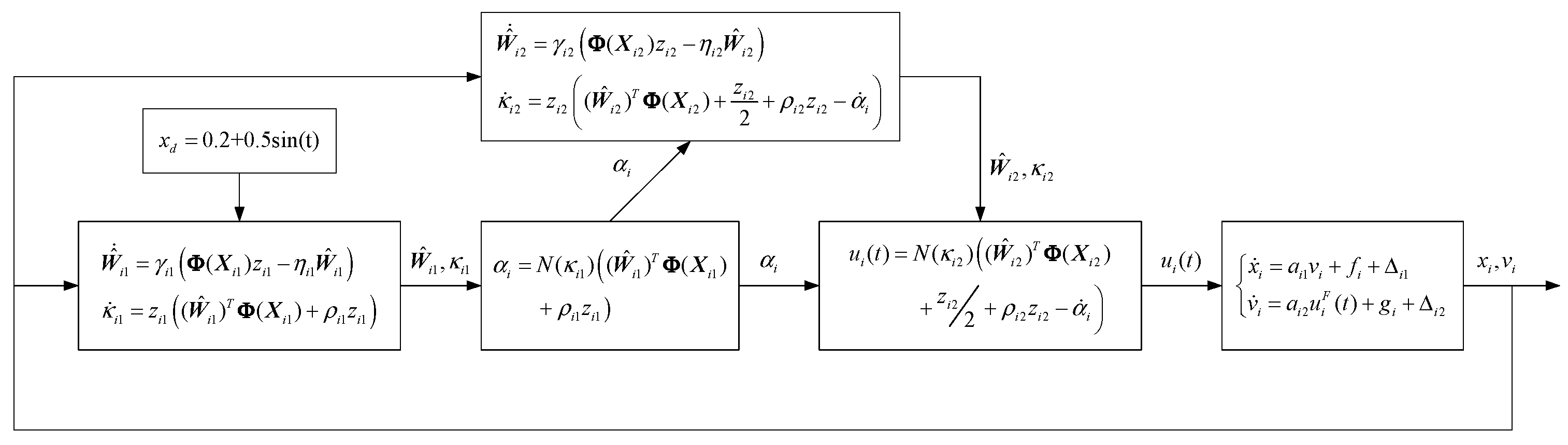
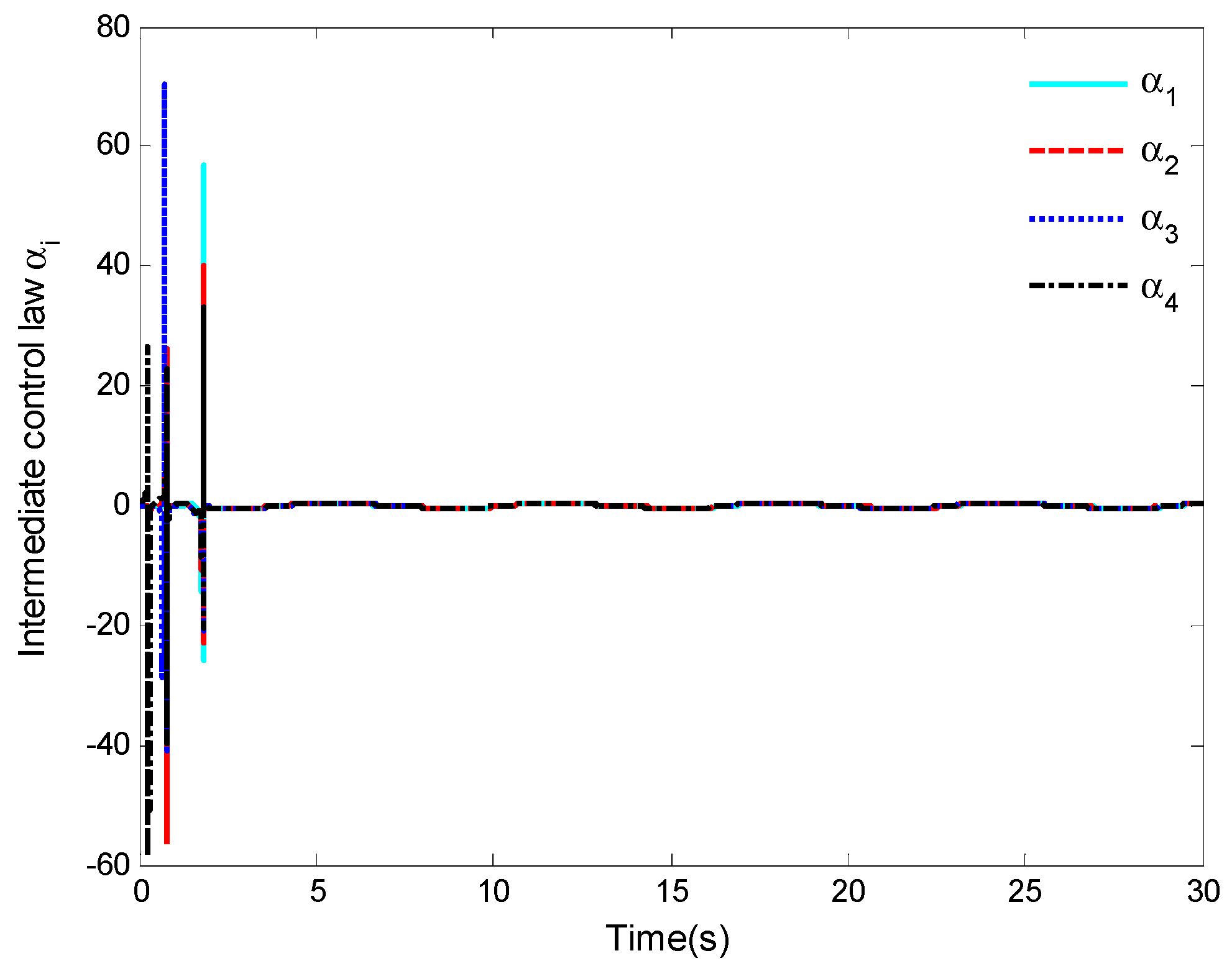
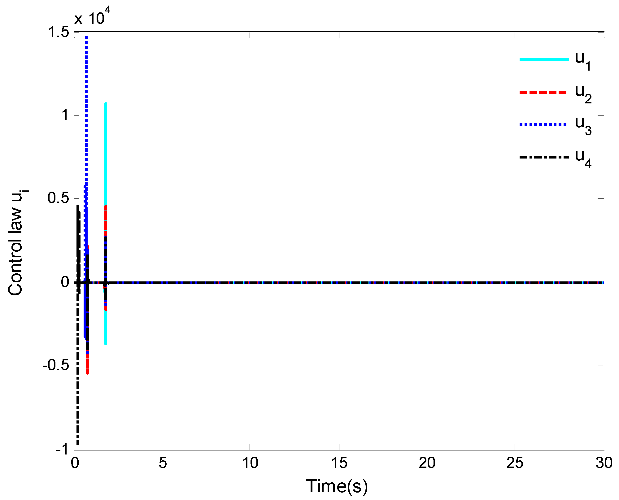
The Nussbaum gain function technology is used in the design of the intermediate control law and of the adaptive fuzzy control law to solve the desired tracking control problem. Compared with [10,24,26,27], the control law designed in this paper can meet the control requirements when the control directions are unknown and coexists with the actuator dead-zone fault.

(iv)

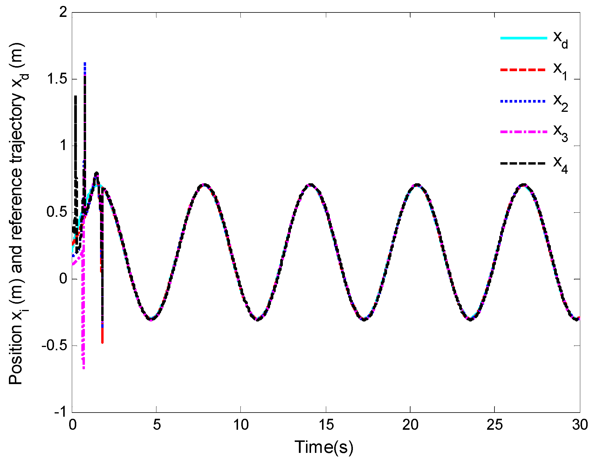
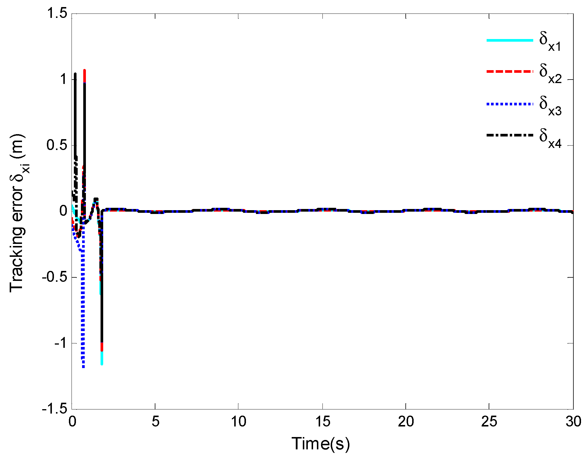
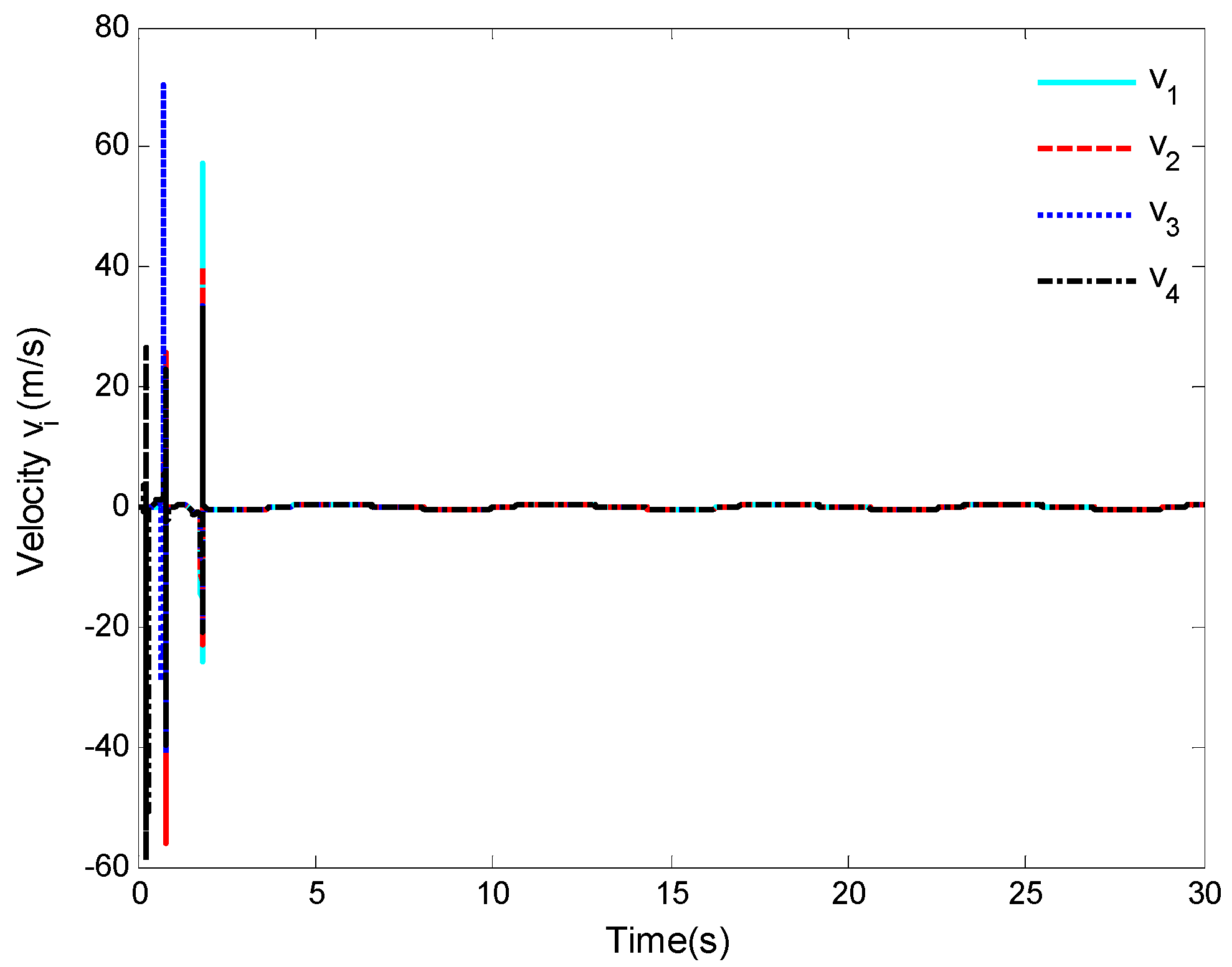
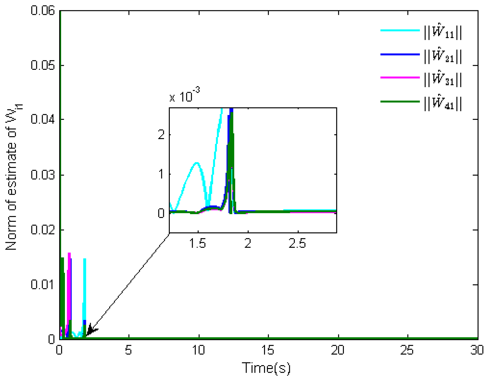
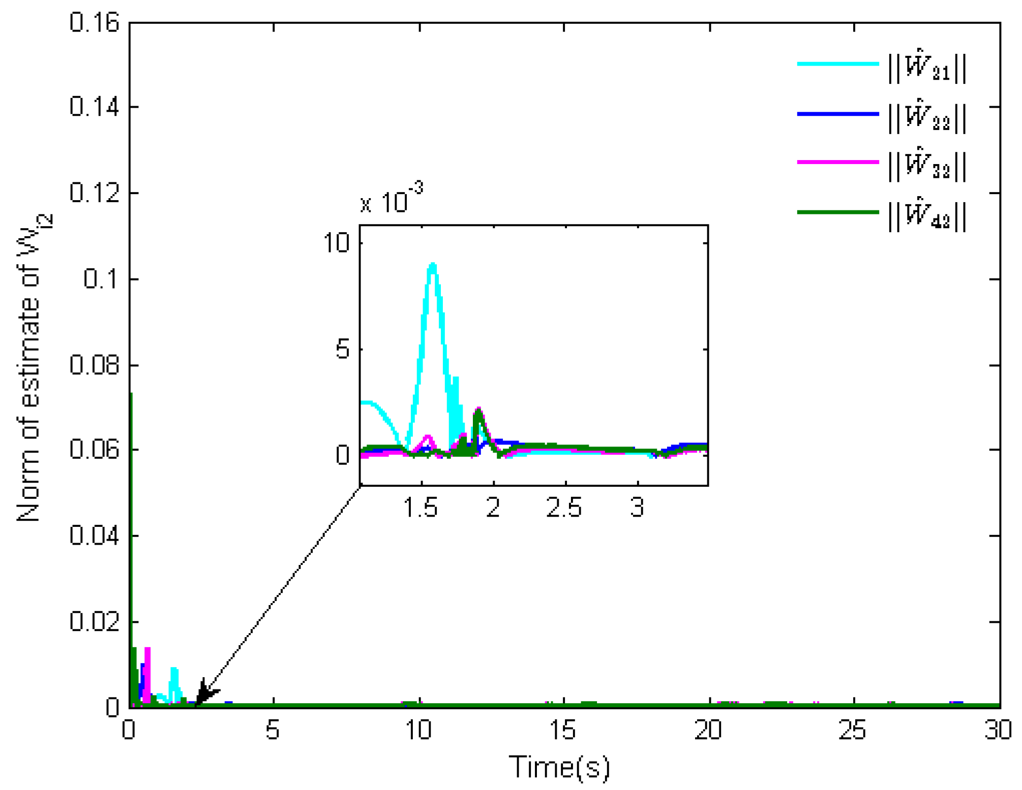
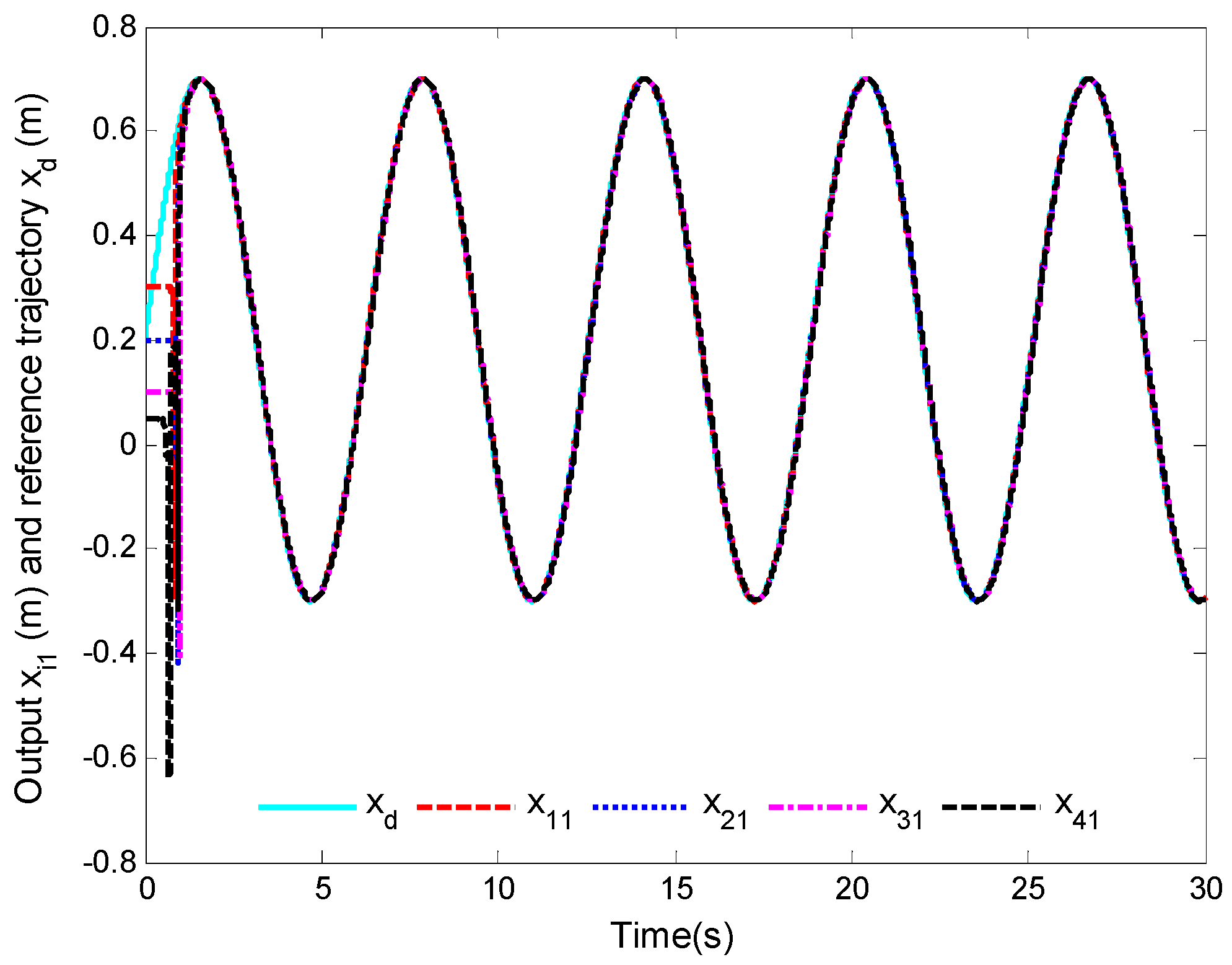
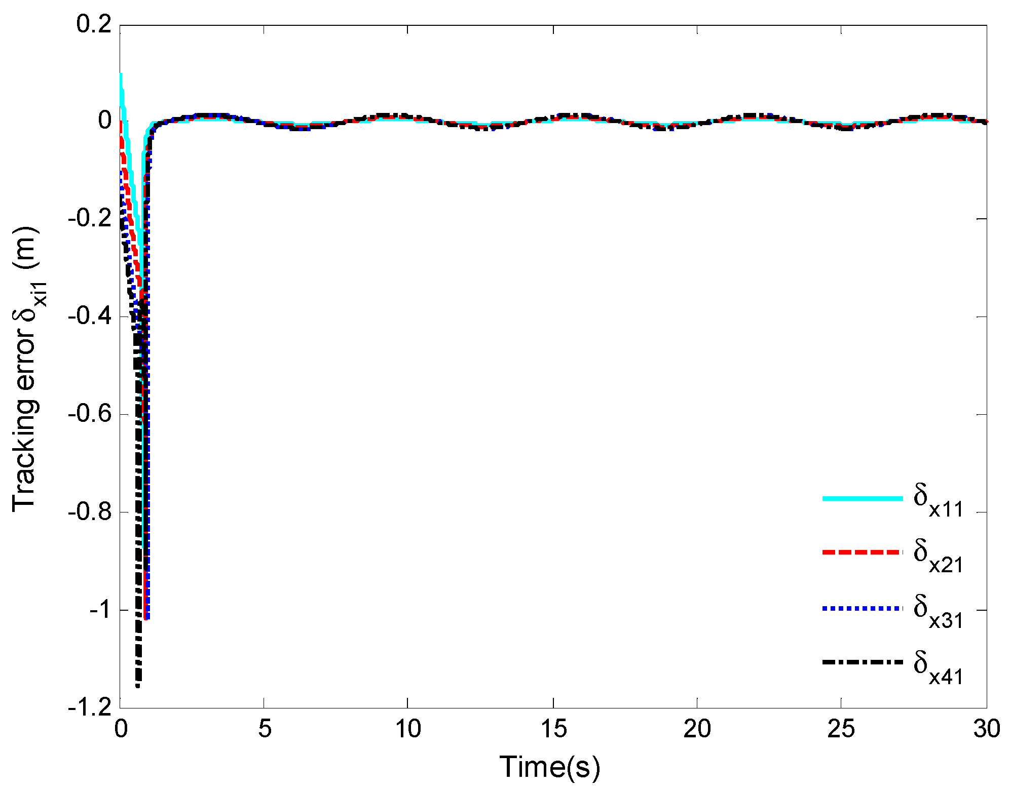
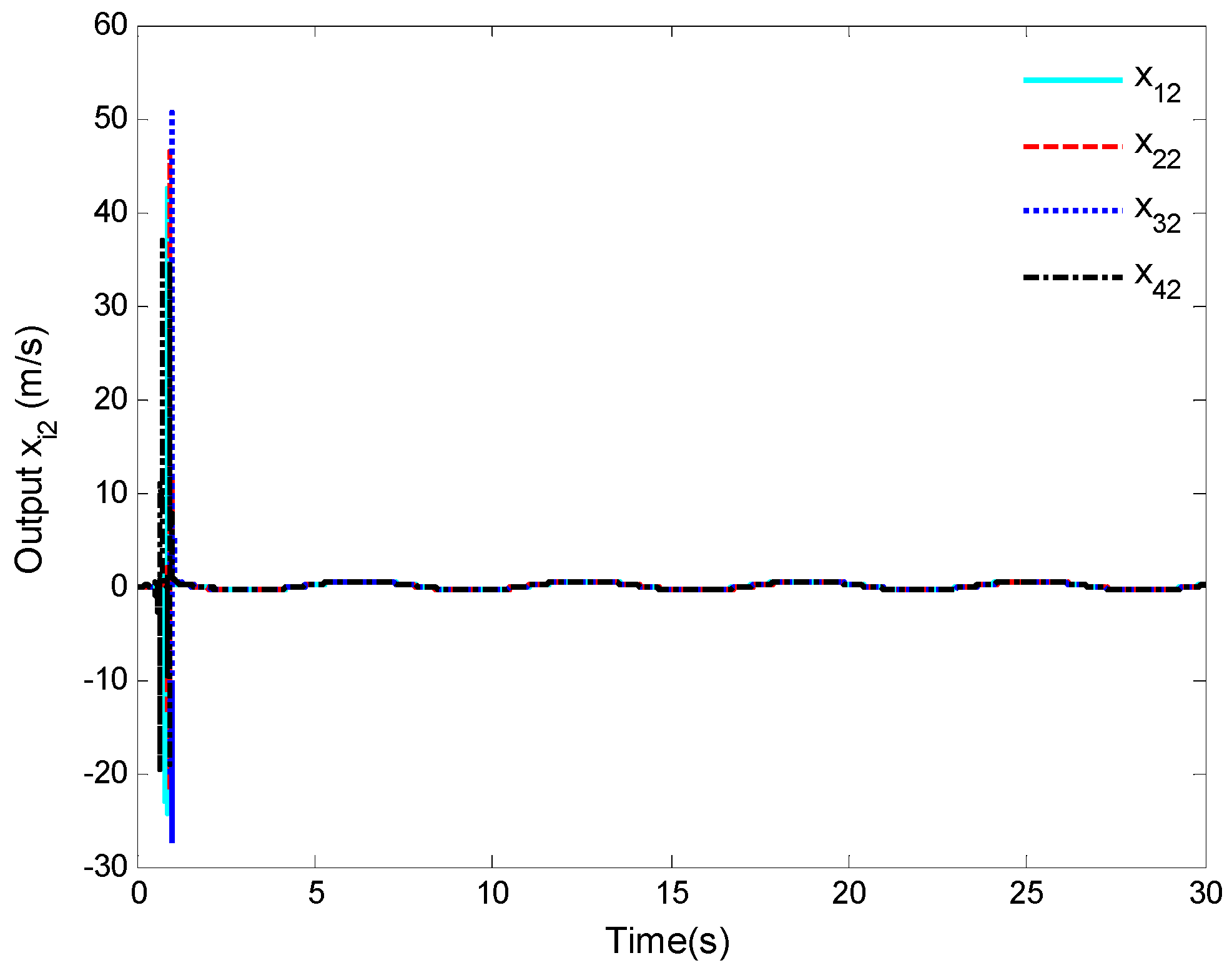
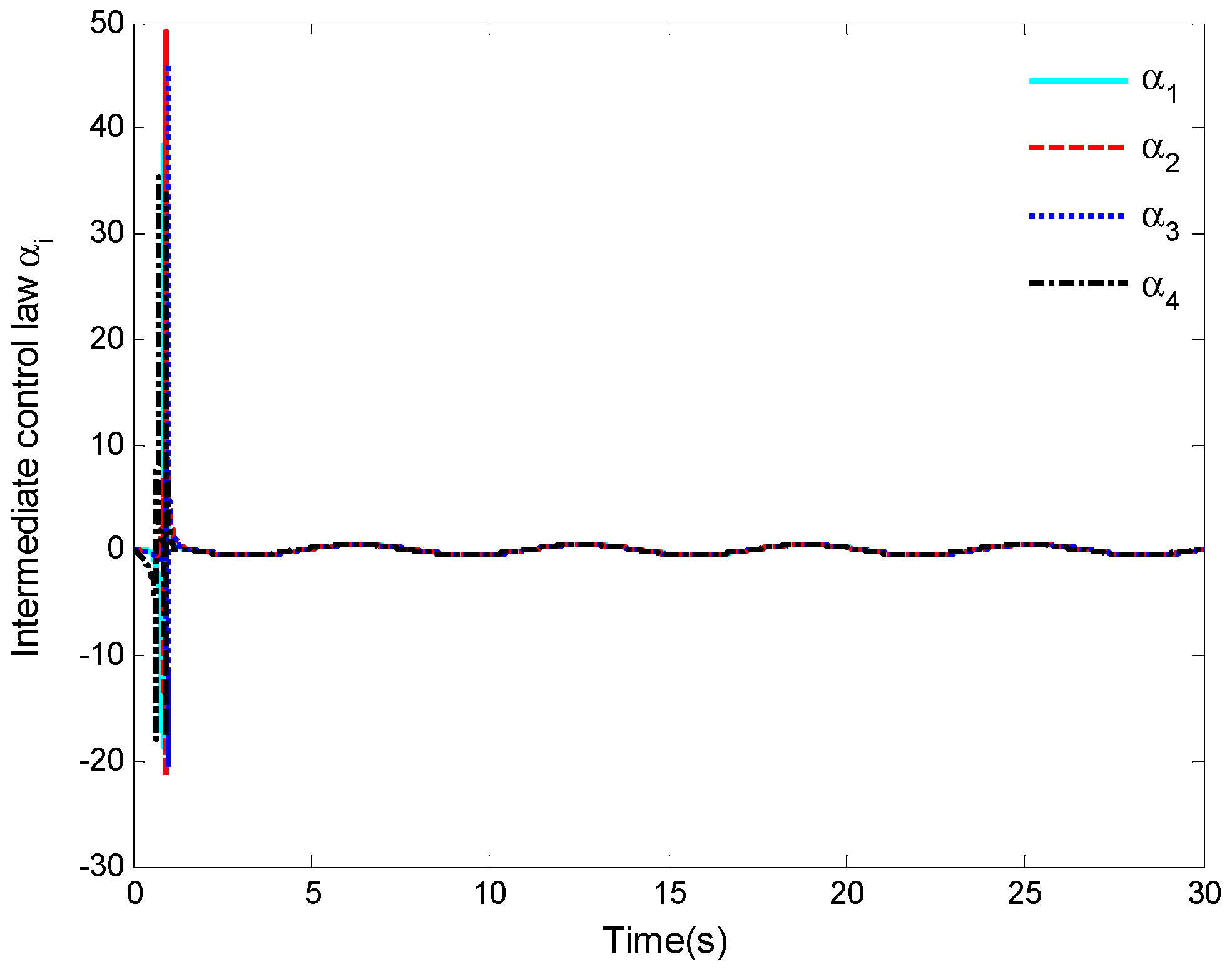
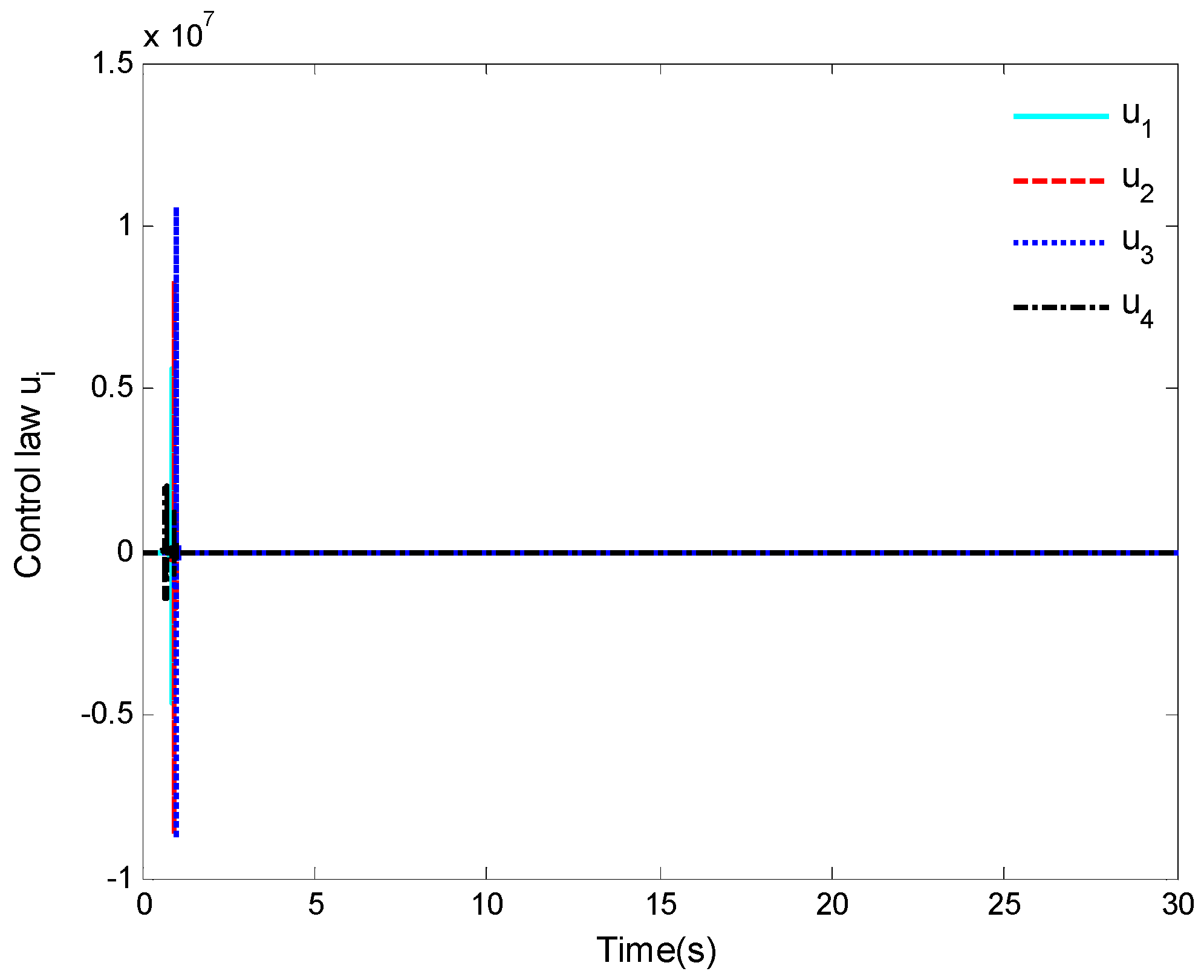
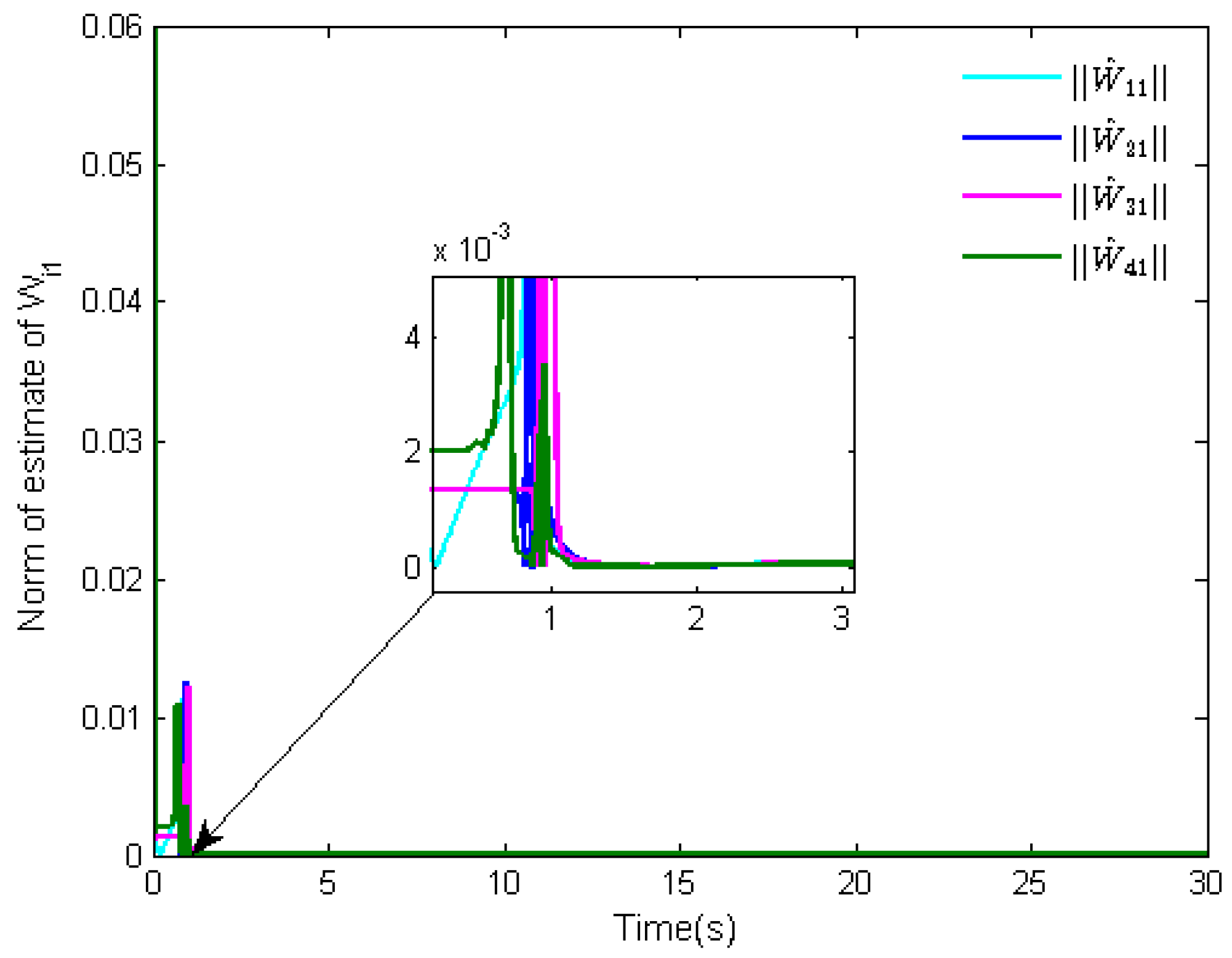
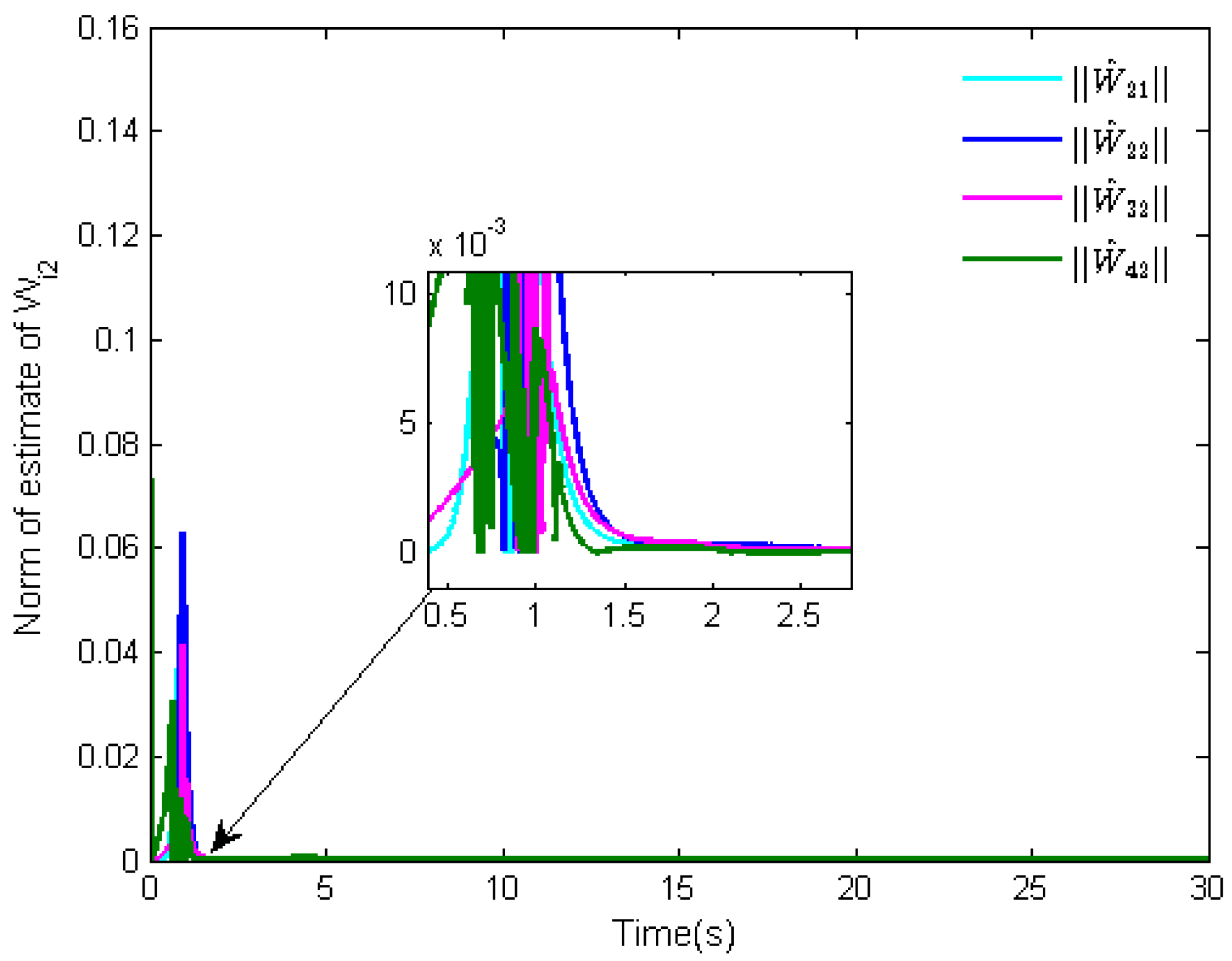
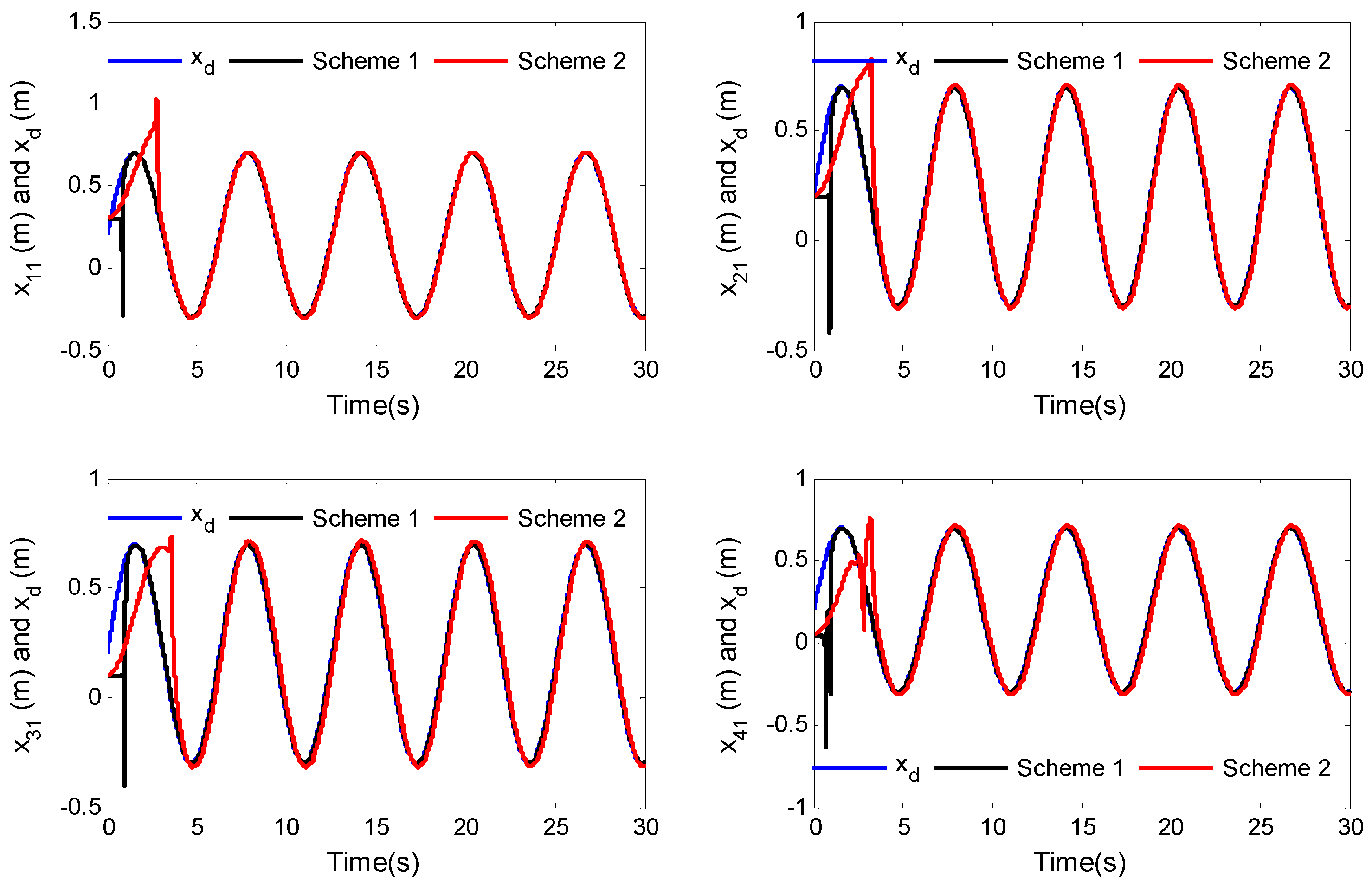
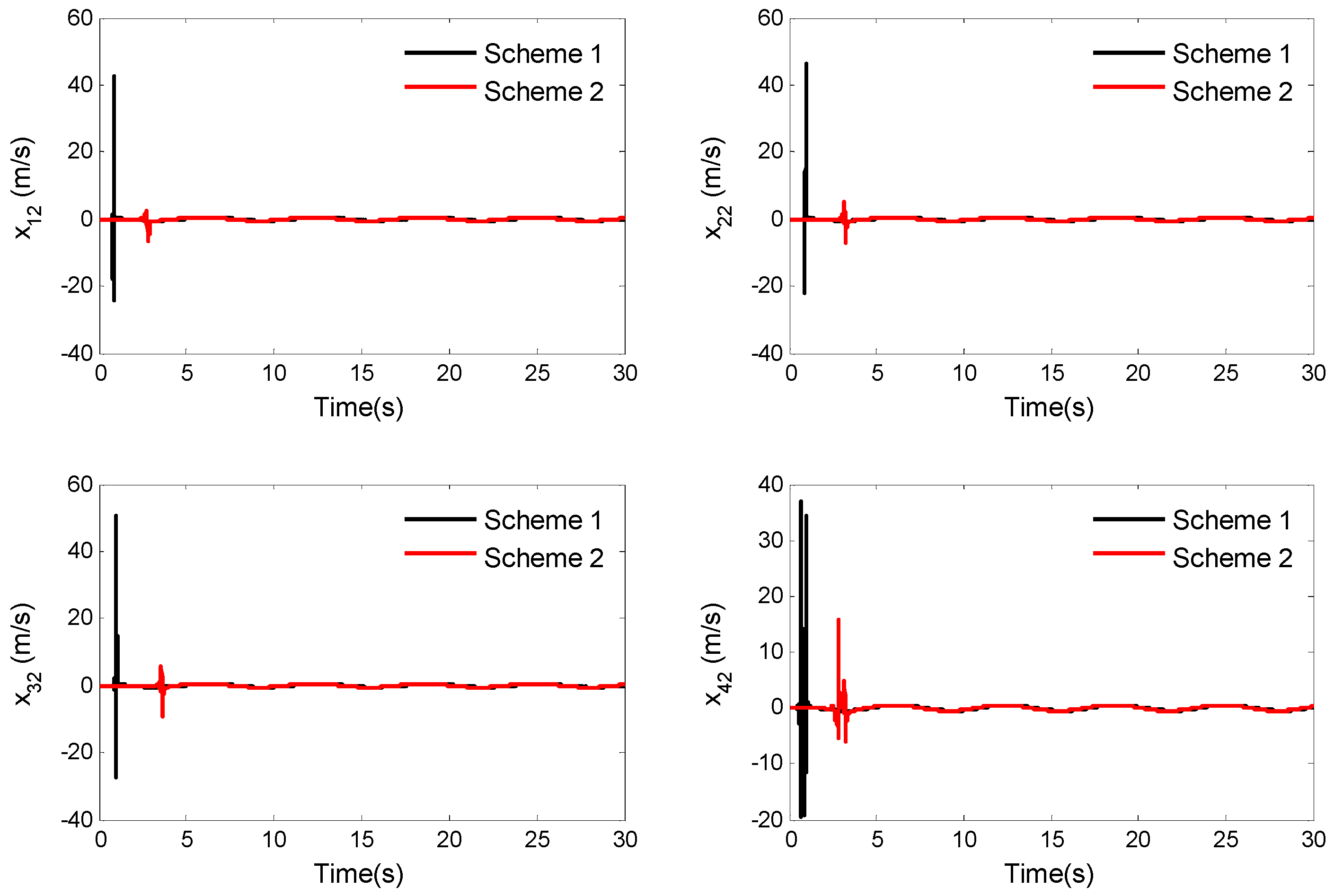
Based on the designed Lyapunov function, the effectiveness of the proposed control law is proven. The simulation results show that the tracking errors can finally converge to a small neighborhood of zero following adjustments to the relevant parameters.

The rest of this paper unfolds as follows: Section 2 introduces the multi-agent systems model, and some preliminaries are given in this section. The main results are provided in Section 3, which mainly involves the design of the adaptive fuzzy control law and the discussion of stability. In Section 4, the simulation analysis is described to illustrate the effectiveness of theoretical results, and the conclusions are briefly drawn in Section 5.

Notations: $\left|A\right|$ stands for the absolute value of constant $A$. $X_{i,\min }$ and $X_{i,\max }$ are the minimum and maximum values of variable $X_i$, respectively. $diag\{x_1,\dots ,x_n\}$ denotes a diagonal matrix with diagonal elements $x_1,\dots ,x_n$. ${(\cdot )}^T$ represents the transposition operation. $\widehat{\mathit{W}}$ is the estimate of $\mathit{W}$, and $\tilde{\mathit{W}}=\mathit{W}-\widehat{\mathit{W}}$ stands for the estimation error. ${\lambda }_{\min }(\cdot )$ and ${\lambda }_{\max }(\cdot )$ represent the smallest and largest eigenvalues of matrix $(\cdot )$.

2. Problem Formulation and Preliminaries

In this section, the problem formulation is provided, and some preliminaries, including graph theory, the fuzzy logic system, and some lemmas, are provided for a subsequent analysis.

2.1. Problem Formulation

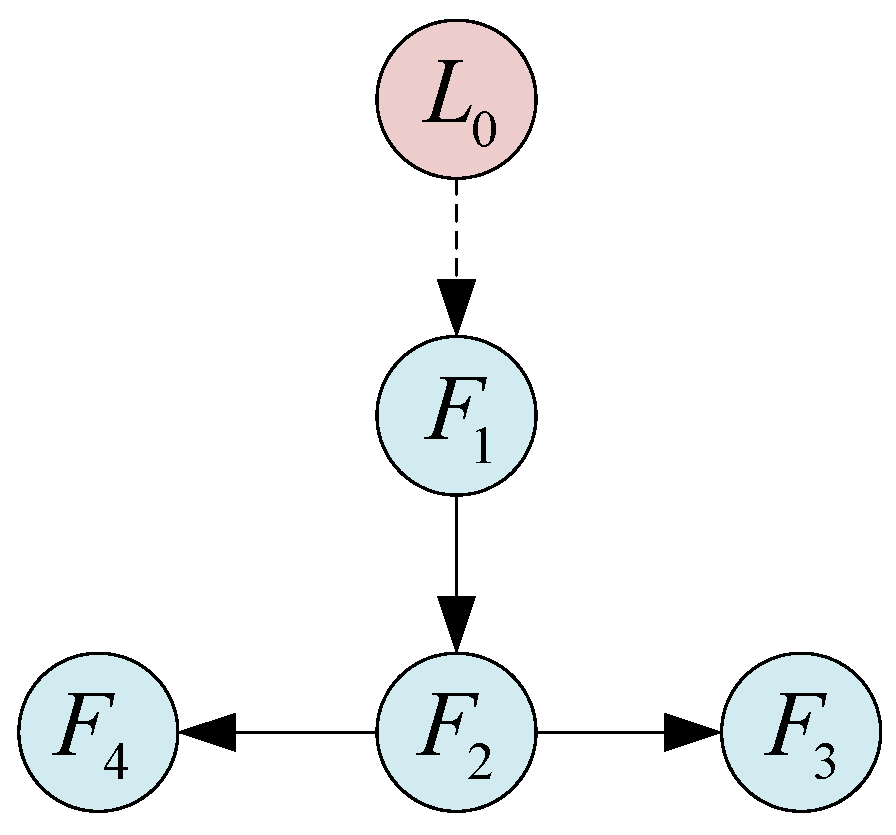
Consider a class of uncertain nonlinear multi-agent systems with unknown control directions and a dead-zone fault, which is composed of one leader agent and $n$ follower agents. The dynamics of follower agent $i$ is described as

$$\left\{\begin{array}{l}{\dot{x}}_i(t)=a_{i1}{v}_i(t)+f_i\left(x_i(t),v_i(t)\right)+{\Delta }_{i1}(t)\\ {\dot{v}}_i(t)=a_{i2}{u}_i^F(t)+g_i\left(x_i(t),v_i(t)\right)+{\Delta }_{i2}(t)\end{array}\right.$$

(1)

where $i=1,\dots ,n$, $x_i(t)$ and $v_i(t)$ represent the position vector and velocity vector; $g_i\left(x_i(t),v_i(t)\right)$ and $f_i\left(x_i(t),v_i(t)\right)$ are unknown smooth nonlinear functions, and for convenience, the functions $g_i\left(x_i(t),v_i(t)\right)$ and $f_i\left(x_i(t),v_i(t)\right)$ are denoted by $g_i$ and $f_i$, respectively; $a_{i1}$ and $a_{i2}$ represent non-zero unknown constants; ${\Delta }_{i1}(t)$ and ${\Delta }_{i2}(t)$ are uncertain dynamics; and $u_i^F(t)$ represents the system input and is supposedly affected by the dead-zone fault. According to [29], the model of a dead-zone fault is:

$$u_i^F(t)=\left\{\begin{array}{l}\omega (u_i(t)-b_{ir}),\hspace{1em}\hspace{0.33em}\hspace{0.33em}\hspace{0.17em}{u}_i(t)\ge b_{ir}\\ \hspace{1em}\hspace{1em}0,\hspace{1em}\hspace{1em}\hspace{1em}-b_{il}<u_i(t)<b_{ir}\\ \omega (u_i(t)+b_{il}),\hspace{1em}\hspace{0.33em}\hspace{0.33em}\hspace{0.17em}{u}_i(t)\le -b_{il}\end{array}\right.$$

(2)

where $\omega >0$ is an unknown bounded constant that represents the slope of the dead-zone; $b_{il}>0$ and $b_{ir}>0$ represent the left and right breakpoints of the dead-zone, respectively. By applying the mean value theorem, (2) can be rewritten as:

$$u_i^F(t)=\omega u_i(t)+{\varphi }_i(t)$$

(3)

where ${\varphi }_i(t)$ is a bounded function and satisfies $\left|{\varphi }_i(t)\right|\le \overline{\varphi }$, and the expression of ${\varphi }_i(t)$ is shown as:

$${\varphi }_i(t)=\left\{\begin{array}{l}-\omega b_{ir},\hspace{1em}\hspace{1em}\hspace{0.33em}\hspace{0.17em}\hspace{0.33em}{u}_i(t)\ge b_{ir}\\ -\omega u_i(t),\hspace{0.33em}-b_{il}<u_i(t)<b_{ir}\\ \omega b_{il},\hspace{1em}\hspace{1em}\hspace{0.33em}\hspace{0.33em}\hspace{0.33em}\hspace{0.33em}\hspace{0.17em}{u}_i(t)\le -b_{il}\end{array}\right.$$

(4)

The objective of this paper is to design an adaptive fuzzy control law $u_i(t)$ for the system (1), so that the output of each follower agent can track the trajectory of the leader agent when the control directions are unknown and an actuator dead-zone fault occurs, and the tracking error of each follower agent can converge to a small neighborhood of zero.

Assumption 1. 

The unknown constants$a_{i1}$and$a_{i2}$are bounded; that is, there exist$0<a_{1,\min }\le \left|a_{i1}\right|\le a_{1,\max }$and$0<a_{2,\min }\le \left|a_{i2}\right|\le a_{2,\max }$. To not lose generality, we further assume that$a_{1,\min }\le a_{i1}\le a_{1,\max }$and$a_{2,\min }\le a_{i2}\le a_{2,\max }$.

Assumption 2.

The uncertain dynamics${\Delta }_{i1}(t)$and${\Delta }_{i2}(t)$are bounded and satisfy$\left|{\Delta }_{i1}(t)\right|\le {\Delta }_{i1}^{\ast }$and$\left|{\Delta }_{i2}(t)\right|\le {\Delta }_{i2}^{\ast }$.

2.2. Graph Theory

Let $\mathcal{G}=(\mathcal{V},\mathcal{E},\mathcal{A})$ denote a directed graph with $n$ nodes, where $\mathcal{V}=\left\{v_1,\dots ,v_n\right\}$ is the set of vertices, $\mathcal{E}=\{(i,j),i,j\in \mathcal{V},\hspace{0.17em}\mathrm{and}\hspace{0.17em}i\ne j\}$ is the set of edges, and $\mathcal{A}=[a_{ij}]\in R^{n\times n}$ is the weighted adjacency matrix of $\mathcal{G}$. If there is an edge between node $i$ and $j$, then $a_{ij}=a_{ji}\ne 0$, and otherwise, $a_{ij}=a_{ji}=0$. The set of neighbors of node $i$ is denoted by ${\mathcal{N}}_i=\{v_j:(v_i,v_j)\in \mathcal{E}\}$. The Laplacian matrix of $\mathcal{G}$ is denoted by $\mathcal{L}=\mathcal{D}-\mathcal{A}$, where $\mathcal{D}=diag\{d_1,\dots d_n\}$ with $d_i={\displaystyle {\sum }_{j=1}^{{\mathcal{N}}_i}{a}_{ij}}$. The graph $\mathcal{G}$ is connected if there is a path between any two vertices.

An extended graph is defined as $\overline{\mathcal{G}}=(\overline{\mathcal{V}},\overline{\mathcal{E}})$, which is associated with the leader agent and follower agents. Let the leader adjacency matrix be $\mathcal{B}=\mathrm{diag}\left\{b_1,\dots ,b_n\right\}$, and if the follower agent $i$ obtains the information of leader agent, then $b_i=1$; otherwise, $b_i=0$.

Assumption 3

[38]. The directed graph $\overline{\mathcal{G}}$ contains a spanning tree, and the leader node is the root node.

2.3. Fuzzy Logic System

In the subsequent analysis, the fuzzy logic system is considered to approximate unknown uncertain dynamics. The fuzzy rule base is composed of “if-then” rules in the following form:

$$R^l: \mathrm{if} x_1 \mathrm{is} F_1^l,\dots , \mathrm{and} x_n \mathrm{is} F_n^l, \mathrm{then} h \mathrm{is} G^l, l=1,\dots ,M,$$

where $x_i$, $i=1,\dots ,n$, and $h$ are the fuzzy logic system’s input and output, respectively; $M$ is the total number of “if-then” rules; $F_1^l,\dots ,F_n^l$ and $G^l$ are fuzzy sets for linguistic variables. Additionally, by applying singleton fuzzifier, product inference, and a defuzzifier [32,39], the fuzzy logic system can be formulated as:

$$h(x)=\frac{{\displaystyle {\sum }_{l=1}^M{\overline{h}}_l{\Pi }_{i=1}^n{\mu }_{F_i^l}(x_i)}}{{\displaystyle {\sum }_{l=1}^M\left[{\Pi }_{i=1}^n{\mu }_{F_i^l}(x_i)\right]}}$$

(5)

where ${\overline{h}}_l={\max }_{h\in R}{\mu }_{G^l}(h)$.

If ${\mathit{W}}^T=\left[{\overline{h}}_1,\dots ,{\overline{h}}_M\right]=\left[w_1,\dots ,w_M\right]$ and $\mathbf{\phi }(x)={\left[{\phi }_1(x),\dots ,{\phi }_M(x)\right]}^T$, then the vector from the fuzzy logic system (5) can be written as:

$$h(x)={\mathit{W}}^T\mathbf{\phi }(x)$$

(6)

where ${\phi }_l(x)=\left({\Pi }_{i=1}^n{\mu }_{F_i^l}(x_i)\right)/\left({\displaystyle {\sum }_{l=1}^M\left[{\Pi }_{i=1}^n{\mu }_{F_i^l}(x_i)\right]}\right)$, $l=1,\dots ,M$; $x={\left[x_1,\dots ,x_n\right]}^T$ is the input of the fuzzy logic system.

Lemma 1

[21]. For any continuous function $f(x)$ defined on a compact set $\Omega$ and any given positive constant $\epsilon$, there exists a fuzzy logic system $f^{\ast }(x)={\mathit{W}}^{\ast T}\mathbf{\phi }(x)$ in the form of (15) such that

$$\underset{x\in \Omega }{\sup }\left|f^{\ast }(x)-f(\mathit{W},\mathbf{\phi })\right|\le \epsilon$$

(7)

where $W^{\ast }$ is the ideal parameter vector, and $\epsilon$ is the approximation accuracy and can be arbitrarily small.

2.4. Definition and Lemmas

Definition 1

[21]. The smooth continuous function $N(\kappa )$ is called the Nussbaum gain function if the following properties hold:

$$\left\{\begin{array}{l}\underset{s\to \infty }{\lim }\sup \frac{1}{s}{\displaystyle {\int }_0^{s}N(\kappa )d}\kappa =+\infty \\ \underset{s\to \infty }{\lim }\inf \frac{1}{s}{\displaystyle {\int }_0^{s}N(\kappa )d}\kappa =-\infty \end{array}\right.$$

(8)

Lemma 2

[21]. Let $V(t)$ and $\kappa (t)$ be smooth functions defined on $[0,t_f)$ with $V(t)\ge 0$, and $N(\kappa )$ be a Nussbaum gain function. If the following inequality holds:

$$V(t)\le e^{-k_{0}t}{\displaystyle {\int }_0^t{e}^{k_0\tau }\left(G({\overline{x}}_n)N(\kappa )+1\right)}\dot{\kappa }(\tau )d\tau +c_0,\hspace{0.33em}t\in [0,t_f)$$

(9)

then $V(t)$, $\kappa (t)$, and ${\displaystyle {\int }_0^t{e}^{k_0\tau }\left(G({\overline{x}}_n)N(\kappa )+1\right)}\dot{\kappa }(\tau )d\tau$ are bounded by $[0,t_f)$, where $G({\overline{x}}_n)$ satisfies $G_m\le \left|G({\overline{x}}_n)\right|\le G_M$ with ${\overline{x}}_n$ being the system state vector, and $G_m$, $G_M$, $c_0$, and $k_0$ are positive constants.

Lemma 3

[15]. For any $x\in R$ and $y\in R$, the following inequality holds:

$$xy\le \frac{{\varsigma }^p}{p}{\left|x\right|}^p+\frac{1}{q{\varsigma }^q}{\left|y\right|}^q$$

(10)

where $\varsigma >0$, $p>1$, $q>1$, and $(p-1)(q-1)=1$.

Lemma 4.

[5]. For any $b\in R$ and $\vartheta >0$, the hyperbolic tangent function satisfies:

$$0\le \left|b\right|-b\tanh (\frac{b}{\vartheta })\le 0.2785\vartheta$$

(11)

3. Adaptive Control Law Design and Stability Analysis

In order to solve the tracking control problem of an uncertain nonlinear multi-agent system (1) with unknown control directions and a dead-zone fault, in this section, the fuzzy logic system and Nussbaum gain function technology are introduced to design the adaptive fuzzy control law, intermediate control law, and adaptive control laws.

3.1. Adaptive Fuzzy Control Law Design

Considering the system (1), the consensus tracking error $z_{i1}$ and velocity tracking error $z_{i2}$, respectively, are defined by:

$$z_{i1}={\displaystyle \sum _{j\in {\mathcal{N}}_i}{a}_{ij}(x_i-x_j)+b_i(x_i-x_d)}$$

(12)

$$z_{i2}=v_i-{\alpha }_i$$

(13)

where $x_d$ represents the trajectory of the leader agent, and ${\alpha }_i$ is the intermediate control law to be designed.

Let ${\delta }_{xi}=x_i-x_d$ stand for the position tracking error of the $i\mathrm{th}$ follower agent, then the vector form of (12) is written as:

$$Z_1=\mathcal{H}{\delta }_x$$

(14)

where $Z_1={[z_{11},\dots ,z_{n1}]}^T$, $\mathcal{H}=\mathcal{L}+\mathcal{B}$, ${\delta }_x={[{\delta }_{x1},\dots ,{\delta }_{xn}]}^T=x-1\otimes x_d$ with $x={\left[x_1,\dots ,x_n\right]}^T$ and $1={\left[1,\dots ,1\right]}^T$.

Define the candidate Lyapunov function $V_1$ as:

$$V_1=\frac{1}{2}{Z}_1^T{\mathcal{H}}^{-1}{Z}_1$$

(15)

According to (12)–(14), the time derivative of $V_1$ is:

$$\begin{array}{l}{\dot{V}}_1=Z_1^T{\mathcal{H}}^{-1}\mathcal{H}{\dot{\delta }}_x\\ \hspace{1em}={\displaystyle \sum _{i=1}^n\left[a_{i1}{z}_{i1}{\alpha }_i+a_{i1}{z}_{i1}{z}_{i2}+z_{i1}\left(f_i+{\Delta }_{i1}-{\dot{x}}_d\right)\right]}\end{array}$$

(16)

Considering Lemma 3 and letting $\varsigma =1$, $p=2$, $q=2$, $x=a_{i1}{z}_{i1}$, and $y=z_{i2}$, we have:

$$a_{i1}{z}_{i1}{z}_{i2}\le \frac{{\left(a_{i1}{z}_{i1}\right)}^2}{2}+\frac{z_{i2}^2}{2}$$

(17)

Substituting (17) into (16) yields:

$${\dot{V}}_1\le {\displaystyle \sum _{i=1}^n\left[a_{i1}{z}_{i1}{\alpha }_i+z_{i1}\left(F_{i1}+{\Delta }_{i1}-{\dot{x}}_d\right)+\frac{z_{i2}^2}{2}\right]}$$

(18)

where $F_{i1}=a_{i1}^2{z}_{i1}/2+f_i$, a fuzzy logic system is introduced to approximate $F_{i1}$, then we obtain:

$$F_{i1}={({\mathit{W}}_{i1}^{\ast })}^T\mathbf{\phi }(X_{i1})+{\epsilon }_{i1}$$

(19)

where $X_{i1}={\left[x_i,v_i,x_j,x_d\right]}^T$, $i=1,\dots ,n$, $j\in {\mathcal{N}}_i$, and ${\epsilon }_{i1}$ is the approximation error.

Noting Assumption 2 and Lemma 1, then there exists

$$\left|{\epsilon }_{i1}+{\Delta }_{i1}\right|\le {\epsilon }_{i1}^{\ast }$$

(20)

where ${\epsilon }_{i1}^{\ast }$ is an unknown positive constant.

Let

$${({\mathit{W}}_{i1})}^T\mathbf{\Phi }(X_{i1})={({\mathit{W}}_{i1}^{\ast })}^T\mathbf{\phi }(X_{i1})+{\epsilon }_{i1}^{\ast }\tanh (\frac{{\epsilon }_{i1}^{\ast }{z}_{i1}}{\vartheta })-{\dot{x}}_d$$

(21)

where

$${\mathit{W}}_{i1}^T=\left[{\mathit{W}}_{i1}^{\ast },1\right]$$

(22)

$$\mathbf{\Phi }(X_{i1})={\left[\mathbf{\phi }(X_{i1}),{\delta }_{i1}^{\ast }\tanh (\frac{{\delta }_{i1}^{\ast }{z}_{i1}}{\vartheta })-{\dot{x}}_d\right]}^T$$

(23)

Substituting (19) and (21) into (18), we have:

$$\begin{array}{l}{\dot{V}}_1\le {\displaystyle \sum _{i=1}^n\left[a_{i1}{z}_{i1}{\alpha }_i+z_{i1}\left({({\mathit{W}}_{i1}^{\ast })}^T\mathbf{\phi }(X_{i1})+{\epsilon }_{i1}+{\Delta }_{i1}-{\dot{x}}_d\right)+\frac{z_{i2}^2}{2}\right]}\\ \hspace{1em}={\displaystyle \sum _{i=1}^n\left[a_{i1}{z}_{i1}{\alpha }_i+z_{i1}\left({({\mathit{W}}_{i1})}^T\mathbf{\Phi }(X_{i1})+{\epsilon }_{i1}+{\Delta }_{i1}-{\epsilon }_{i1}^{\ast }\tanh (\frac{{\epsilon }_{i1}^{\ast }{z}_{i1}}{\vartheta })\right)+\frac{z_{i2}^2}{2}\right]}\end{array}$$

(24)

The intermediate control law ${\alpha }_i$ and adaptive control law ${\dot{\kappa }}_{i1}$ are designed as follows:

$${\alpha }_i=N({\kappa }_{i1})\left({({\widehat{\mathit{W}}}_{i1})}^T\mathbf{\Phi }(X_{i1})+{\rho }_{i1}{z}_{i1}\right)$$

(25)

$${\dot{\kappa }}_{i1}=z_{i1}\left({({\widehat{\mathit{W}}}_{i1})}^T\mathbf{\Phi }(X_{i1})+{\rho }_{i1}{z}_{i1}\right)$$

(26)

where ${\widehat{\mathit{W}}}_{i1}$ represents the estimate of ${\mathit{W}}_{i1}$, and ${\rho }_{i1}$ is the positive constant to be designed.

Considering Lemma 4, one obtains $({\epsilon }_{i1}+{\Delta }_{i1})-{\epsilon }_{i1}^{\ast }\tanh ({\epsilon }_{i1}^{\ast }{z}_{i1}/\vartheta )\le 0.2785\vartheta$; then, substituting (25) and (26) into (24), we have:

$$\begin{array}{l}{\dot{V}}_1\le {\displaystyle \sum _{i=1}^n\left[\left(a_{i1}N({\kappa }_{i1}){\dot{\kappa }}_{i1}+{\dot{\kappa }}_{i1}\right)-{\rho }_{i1}{z}_{i1}^2+z_{i1}{({\tilde{{W}}}_{i1})}^T\mathbf{>\Phi }(X_{i1})+z_{i1}({\epsilon }_{i1}+{\Delta }_{i1})-z_{i1}{\epsilon }_{i1}^{\ast }\tanh (\frac{{\epsilon }_{i1}^{\ast }{z}_{i1}}{\vartheta })+\frac{z_{i2}^2}{2}\right]}\\ \hspace{1em}\le {\displaystyle \sum _{i=1}^n\left[\left(a_{i1}N({\kappa }_{i1}){\dot{\kappa }}_{i1}+{\dot{\kappa }}_{i1}\right)-{\rho }_{i1}{z}_{i1}^2+z_{i1}{({\tilde{\mathit{W}}}_{i1})}^T\mathbf{\Phi }(X_{i1})+\frac{z_{i2}^2}{2}+0.2785\vartheta \right]}\end{array}$$

(27)

where ${\tilde{\mathit{W}}}_{i1}={\mathit{W}}_{i1}-{\widehat{\mathit{W}}}_{i1}$.

With reference to the description in [40], the adaptive control law ${\dot{\widehat{\mathit{W}}}}_{i1}$ can be designed as:

$${\dot{\widehat{\mathit{W}}}}_{i1}={\gamma }_{i1}\left(\mathbf{\Phi }(X_{i1})z_{i1}-{\eta }_{i1}{\widehat{W}}_{i1}\right)$$

(28)

where ${\gamma }_{i1}$ and ${\eta }_{i1}$ are designed as positive constants.

Furthermore, the candidate Lyapunov function $V_2$ is defined as:

$$V_2=\frac{1}{2}{Z}_2^T{Z}_2$$

(29)

where $Z_2={[z_{12},\dots ,z_{n2}]}^T$.

With reference to (3) and (13), the time derivative of $V_2$ is:

$$\begin{array}{l}{\dot{V}}_2={\displaystyle \sum _{i=1}^n{z}_{i2}\left({\dot{v}}_i-{\dot{\alpha }}_i\right)}\\ \hspace{1em}={\displaystyle \sum _{i=1}^n{z}_{i2}\left(a_{i2}(\omega u_i(t)+{\varphi }_i(t))+g_i+{\Delta }_{i2}-{\dot{\alpha }}_i\right)}\\ \hspace{1em}={\displaystyle \sum _{i=1}^n\left(\omega a_{i2}{z}_{i2}{u}_i(t)+a_{i2}{\varphi }_i(t)z_{i2}+z_{i2}(g_i+{\Delta }_{i2})-z_{i2}{\dot{\alpha }}_i\right)}\end{array}$$

(30)

Similarly, considering Lemma (3), we have:

$$a_{i2}{\varphi }_i(t)z_{i2}\le \frac{{(a_{i2}{z}_{i2})}^2}{2}+\frac{{\varphi }_i{}^2(t)}{2}$$

(31)

Substituting (31) into (30) obtains:

$${\dot{V}}_2\le {\displaystyle \sum _{i=1}^n\left(\omega a_{i2}{z}_{i2}{u}_i(t)+z_{i2}\left(F_{i2}+{\Delta }_{i2}\right)-z_{i2}{\dot{\alpha }}_i+\frac{{\varphi }_i^2(t)}{2}\right)}$$

(32)

where $F_{i2}=a_{i2}^2{z}_{i2}/2+g_i$, and a fuzzy logic system is introduced to approximate $F_{i2}$; then, we obtain:

$$F_{i2}={({\mathit{W}}_{i2}^{\ast })}^T\mathbf{\phi }(X_{i2})+{\epsilon }_{i2}$$

(33)

where $X_{i2}={\left[x_i,v_i,x_j,x_d\right]}^T$, $i=1,\dots ,n$, $j\in {\mathcal{N}}_i$, and ${\epsilon }_{i2}$ stands for the approximation error.

Noting Assumption 2 and Lemma 1, we have:

$$\left|{\epsilon }_{i2}+{\Delta }_{i2}\right|\le {\epsilon }_{i2}^{\ast }$$

(34)

where ${\epsilon }_{i2}^{\ast }$ is an unknown positive constant.

Let

$${({\mathit{W}}_{i2})}^T\mathsf{\Phi }(X_{i2})={({\mathit{W}}_{i2}^{\ast })}^T\mathbf{\phi }(X_{i2})+{\epsilon }_{i2}^{\ast }\tanh (\frac{{\epsilon }_{i2}^{\ast }{z}_{i2}}{\vartheta })$$

(35)

where

$${\mathit{W}}_{i2}^T=\left[{\mathit{W}}_{i2}^{\ast },1\right]$$

(36)

$$\mathsf{\Phi }(X_{i2})={\left[\mathbf{\phi }(X_{i2}),{\delta }_{i2}^{\ast }\tanh (\frac{{\delta }_{i2}^{\ast }{z}_{i2}}{\vartheta })\right]}^T$$

(37)

Furthermore, substituting (33) and (35) into (32) yields:

$$\begin{array}{l}{\dot{V}}_2\le {\displaystyle \sum _{i=1}^n\left(\omega a_{i2}{z}_{i2}{u}_i(t)+z_{i2}\left({({\mathit{W}}_{i2}^{\ast })}^T\mathit{\phi }(X_{i2})+{\epsilon }_{i2}+{\Delta }_{i2}\right)-z_{i2}{\dot{\alpha }}_i+\frac{{\varphi }_i^2(t)}{2}\right)}\\ \hspace{1em}={\displaystyle \sum _{i=1}^n\left[\omega a_{i2}{z}_{i2}{u}_i+z_{i2}\left({({\mathit{W}}_{i2})}^T\mathbf{\Phi }(X_{i2})+({\epsilon }_{i2}+{\Delta }_{i2})-{\epsilon }_{i2}^{\ast }\tanh (\frac{{\epsilon }_{i2}^{\ast }{z}_{i2}}{\vartheta })\right)-z_{i2}{\dot{\alpha }}_i+\frac{{\varphi }_i^2(t)}{2}\right]}\end{array}$$

(38)

The adaptive fuzzy control law $u_i(t)$ and adaptive control law ${\dot{\kappa }}_{i2}$ are designed as follows:

$$u_i(t)=N({\kappa }_{i2})\left({({\widehat{\mathit{W}}}_{i2})}^T\mathbf{\Phi }(X_{i2})+\frac{z_{i2}}{2}+{\rho }_{i2}{z}_{i2}-{\dot{\alpha }}_i\right)$$

(39)

$${\dot{\kappa }}_{i2}=z_{i2}\left({({\widehat{W}}_{i2})}^T\mathbf{\Phi }(X_{i2})+\frac{z_{i2}}{2}+{\rho }_{i2}{z}_{i2}-{\dot{\alpha }}_i\right)$$

(40)

where ${\widehat{\mathit{W}}}_{i2}$ represents the estimate of ${\mathit{W}}_{i2}$, and ${\rho }_{i2}$ is the positive constant to be designed.

By substituting (39) and (50) into (38), and considering Lemma 4, we have:

$${\dot{V}}_2\le {\displaystyle \sum _{i=1}^n\left((\omega a_{i2}N({\kappa }_{i2}){\dot{\kappa }}_{i2}+{\dot{\kappa }}_{i2})-{\rho }_{i2}{z}_{i2}^2+z_{i2}{({\tilde{\mathit{W}}}_{i2})}^T\mathbf{\Phi }(X_{i2})-\frac{z_{i2}^2}{2}+\frac{{\varphi }_i^2(t)}{2}+0.2785\vartheta \right)}$$

(41)

where ${\tilde{\mathit{W}}}_{i2}={\mathit{W}}_{i2}-{\widehat{\mathit{W}}}_{i2}$.

Similarly, we design the adaptive control law ${\dot{\widehat{\mathit{W}}}}_{i2}$ as:

$${\dot{\widehat{\mathit{W}}}}_{i2}={\gamma }_{i2}\left(\mathbf{\Phi }(X_{i2})z_{i2}-{\eta }_{i2}{\widehat{\mathit{W}}}_{i2}\right)$$

(42)

where ${\gamma }_{i2}$ and ${\eta }_{i2}$ are the designed positive constants.

3.2. Stability Analysis

In order to verify the validity of the proposed adaptive fuzzy control law, the following theorem is provided.

Theorem 1.

Consider the uncertain nonlinear multi-agent systems (1) with unknown control directions and dead-zone fault under Assumptions 1–3, and the intermediate control law (25), adaptive control laws (26), (28), (40), and (42), and adaptive fuzzy control law (39) are applied such that the system (1) can track the trajectory of the leader agent, and the tracking errors of all follower agents finally converge to a small neighborhood of zero.

Proof. 

We design the Lyapunov function $V$ as:

$$V=V_1+V_2+{\displaystyle \sum _{i=1}^n\frac{{({\tilde{\mathit{W}}}_{i1})}^T{\tilde{\mathit{W}}}_{i1}}{2{\gamma }_{i1}}}+{\displaystyle \sum _{i=1}^n\frac{{({\tilde{\mathit{W}}}_{i2})}^T{\tilde{\mathit{W}}}_{i2}}{2{\gamma }_{i2}}}$$

(43)

In combination with (27), (28), (41), and (42), and considering ${\dot{\tilde{\mathit{W}}}}_{i1}=-{\dot{\widehat{\mathit{W}}}}_{i1}$ and ${\dot{\tilde{\mathit{W}}}}_{i2}=-{\dot{\widehat{\mathit{W}}}}_{i2}$, the time derivative of $V$ is given as:

$$\begin{array}{l}\dot{V}\le {\displaystyle \sum _{i=1}^n\left(a_{i1}N({\kappa }_{i1}){\dot{\kappa }}_{i1}+{\dot{\kappa }}_{i1}\right)}+{\displaystyle \sum _{i=1}^n\left(\omega a_{i2}N({\kappa }_{i2}){\dot{\kappa }}_{i2}+{\dot{\kappa }}_{i2}\right)}-{\displaystyle \sum _{i=1}^n\left({\rho }_{i1}{z}_{i1}^2+{\rho }_{i2}{z}_{i2}^2\right)}\\ \hspace{1em}\hspace{0.33em}\hspace{0.33em}+{\displaystyle \sum _{i=1}^n{\eta }_{i1}{({\tilde{\mathit{W}}}_{i1})}^T{\widehat{\mathit{W}}}_{i1}}+{\displaystyle \sum _{i=1}^n{\eta }_{i2}{({\tilde{\mathit{W}}}_{i2})}^T{\widehat{\mathit{W}}}_{i2}}+{\displaystyle \sum _{i=1}^n{D}_i}\end{array}$$

(44)

where $D_i={\varphi }_i^2(t)/2+0557\vartheta$.

Due to

$${({\tilde{\mathit{W}}}_{i1})}^T{\widehat{\mathit{W}}}_{i1}\le -\frac{{({\tilde{\mathit{W}}}_{i1})}^T{\tilde{\mathit{W}}}_{i1}}{2}+\frac{{({\mathit{W}}_{i1})}^T{\mathit{W}}_{i1}}{2}$$

(45)

$${({\tilde{\mathit{W}}}_{i2})}^T{\widehat{\mathit{W}}}_{i2}\le -\frac{{({\tilde{\mathit{W}}}_{i2})}^T{\tilde{\mathit{W}}}_{i2}}{2}+\frac{{({\mathit{W}}_{i2})}^T{\mathit{W}}_{i2}}{2}$$

(46)

By substituting (45) and (46) into (44), we obtain:

$$\begin{array}{l}\dot{V}\le {\displaystyle \sum _{i=1}^n\left(a_{i1}N({\kappa }_{i1}){\dot{\kappa }}_{i1}+{\dot{\kappa }}_{i1}\right)}+{\displaystyle \sum _{i=1}^n\left(\omega a_{i2}N({\kappa }_{i2}){\dot{\kappa }}_{i2}+{\dot{\kappa }}_{i2}\right)}-{\displaystyle \sum _{i=1}^n\left({\rho }_{i1}{z}_{i1}^2+{\rho }_{i2}{z}_{i2}^2\right)}\\ \hspace{1em}\hspace{0.33em}\hspace{0.33em}-\frac{1}{2}{\displaystyle \sum _{i=1}^n{\eta }_{i1}{({\tilde{W}}_{i1})}^T{\tilde{\mathit{W}}}_{i1}}-\frac{1}{2}{\displaystyle \sum _{i=1}^n{\eta }_{i2}{({\tilde{\mathit{W}}}_{i2})}^T{\tilde{\mathit{W}}}_{i2}}+d_0\end{array}$$

(47)

where $d_0=\frac{1}{2}{\displaystyle \sum _{i=1}^n\left({\eta }_{i1}{({\mathit{W}}_{i1})}^T{\mathit{W}}_{i1}+{\eta }_{i2}{({\mathit{W}}_{i2})}^T{\mathit{W}}_{i2}+2D_i\right)}$.

$\sigma$ is chosen so that

$$\sigma =\underset{i=1,\dots ,n}{\min }\left\{2{\rho }_{i1}/{\lambda }_{\max }({\mathcal{H}}^{-1}),2{\rho }_{i2},{\gamma }_{i1}{\eta }_{i1},{\gamma }_{i2}{\eta }_{i2}\right\}$$

(48)

where ${\lambda }_{\max }({\mathcal{H}}^{-1})$ represents the maximum characteristic value of ${\mathcal{H}}^{-1}$.

Thus, (47) can be rewritten as:

$$\dot{V}\le -\sigma V+{\displaystyle \sum _{i=1}^n\left(a_{i1}N({\kappa }_{i1}){\dot{\kappa }}_{i1}+{\dot{\kappa }}_{i1}\right)}+{\displaystyle \sum _{i=1}^n\left(\omega a_{i2}N({\kappa }_{i2}){\dot{\kappa }}_{i2}+{\dot{\kappa }}_{i2}\right)}+d_0$$

(49)

Both sides of (50) are multiplied by $e^{\sigma t}$, and integrated over the interval $[0,t)$; then, we have:

$$\begin{array}{l}V\le e^{-\sigma t}{\displaystyle \sum _{i=1}^n{\displaystyle {\int }_0^t{e}^{\sigma \tau }\left(a_{i1}N({\kappa }_{i1}){\dot{\kappa }}_{i1}+{\dot{\kappa }}_{i1}\right)d\tau }}+e^{-\sigma t}{\displaystyle \sum _{i=1}^n{\displaystyle {\int }_0^t{e}^{\sigma \tau }\left(\omega a_{i2}N({\kappa }_{i2}){\dot{\kappa }}_{i2}+{\dot{\kappa }}_{i2}\right)d\tau }}\\ \hspace{1em}\hspace{0.33em}\hspace{0.33em}+\left(V(0)-\frac{d_0}{\sigma }\right)e^{-\sigma t}+\frac{d_0}{\sigma }\end{array}$$

(50)

According to the previous analysis, the unknown constants $a_{i1}$ and $\omega a_{i2}$ are bounded. Considering Lemma 2, it becomes evident that $V(t)$, ${\displaystyle {\int }_0^t{e}^{\sigma \tau }\left(a_{i1}N({\kappa }_{i1}){\dot{\kappa }}_{i1}+{\dot{\kappa }}_{i1}\right)d\tau }$, ${\displaystyle {\int }_0^t{e}^{\sigma \tau }\left(\omega a_{i2}N({\kappa }_{i2}){\dot{\kappa }}_{i2}+{\dot{\kappa }}_{i2}\right)d\tau }$, and ${\kappa }_{i1}$ and ${\kappa }_{i2}$ for $i=1,\dots ,n$, are bounded over the interval $[0,t)$. Let

$$C=\underset{i=1,\dots ,n}{\max }\left({\displaystyle \sum _{i=1}^n{\displaystyle {\int }_0^t{e}^{\sigma \tau }\left(a_{i1}N({\kappa }_{i1}){\dot{\kappa }}_{i1}+{\dot{\kappa }}_{i1}\right)d\tau }}+{\displaystyle \sum _{i=1}^n{\displaystyle {\int }_0^t{e}^{\sigma \tau }\left(\omega a_{i2}N({\kappa }_{i2}){\dot{\kappa }}_{i2}+{\dot{\kappa }}_{i2}\right)d\tau }}\right)$$

(51)

Then, (50) can be simplified as:

$$V\le \left(V(0)+C-\frac{d_0}{\sigma }\right)e^{-\sigma t}+\frac{d_0}{\sigma }$$

(52)

Considering (14), (15), and (43), for $t\to \infty$, we obtain:

$$\underset{t\to \infty }{\lim }\left|{\delta }_{xi}\right|=\underset{t\to \infty }{\lim }\left|x_i-x_d\right|\le \sqrt{\frac{2d_0}{{\lambda }_{\min }(\mathcal{H})\sigma }}$$

(53)

where ${\lambda }_{\min }(\mathcal{H})$ represents the minimum eigenvalue of $\mathcal{H}$.

By observing (48) and adjusting ${\rho }_{i1}$, ${\rho }_{i2}$, ${\gamma }_{i1}$, ${\gamma }_{i2}$, ${\eta }_{i1}$, and ${\eta }_{i2}$, $\sigma$ is sufficiently large. According to (53), the increase in $\sigma$ or decrease in $d_0$ ensures that the tracking error $\left|{\delta }_{xi}\right|$ converges to a small neighborhood of zero. The proof is completed. □

The control block diagram of the system is given in Figure 1.

Note 1.

Noting (53), the tracking error ${\lim }_{t\to \infty }\left|{\delta }_{xi}\right|\le \sqrt{2d_0/{\lambda }_{\min }(\mathcal{H})\sigma }$ can converge to a small neighborhood of zero by adjusting the parameters of $d_0$ and $\sigma$ . We can decrease $d_0$ by decreasing ${\eta }_{i1}$ and ${\eta }_{i2}$ or increase $\sigma$ by increasing ${\rho }_{i1}$, ${\rho }_{i2}$, ${\gamma }_{i1}$, and ${\gamma }_{i2}$. Nevertheless, the change in these parameters may cause the amplitude of the control signal to become larger. Therefore, to select the appropriate design parameters, a reasonable trade-off should be made between tracking performance and control signal amplitude.

4. Simulation Analysis

In this section, two simulation cases are provided to verify the effectiveness of theoretical analysis results.

Case 1.

Consider the following uncertain nonlinear multi-agent system with unknown control directions and a dead-zone fault:

$$\left\{\begin{array}{l}{\dot{x}}_i(t)=1.5v_i(t)+x_i(t)e^{-1.5x_i(t)}+0.01\sin (t)\\ {\dot{v}}_i(t)=2u^F(t)+0.3\sin (x_i(t))\cos (v_i(t))+0.01\cos (t)\\ i=1,2,3,4\end{array}\right.$$

(54)

The communication topology of the multi-agent systems is shown in Figure 2. Here, $L_0$ represents the leader agent, and $F_1$, $F_2$, $F_3$, and $F_4$ represent the follower agents. The reference trajectory is given as $x_d=0.2+0.5\sin (t)$.

According to Figure 1, we obtain the Laplacian matrix $\mathcal{L}$ and adjacency matrix $\mathcal{B}$ as:

$$\mathcal{L}=\left[\begin{array}{cccc}0& 0& 0& 0\\ -1& 1& 0& 0\\ 0& -1& 1& 0\\ 0& -1& 0& 1\end{array}\right], \mathcal{B}=diag\left\{1,0,0,0\right\}$$

The initial conditions of four follower agents are set as $x_1(0)=0.25(\mathrm{m})$, $x_2(0)=0.15(\mathrm{m})$, $x_3(0)=0.1(\mathrm{m})$, $x_4(0)=0.35(\mathrm{m})$, and $v_1(0)=v_2(0)=v_3(0)=v_4(0)=0(\mathrm{m}/\mathrm{s})$. The model of the actuator dead-zone fault is shown in (2), and the parameters are given as $\omega =1.5$, $b_{ir}=0.3$, and $b_{il}=0.1$.

The fuzzy logic systems are introduced to approximate the uncertain dynamics $F_{i1}=a_{i1}^2{z}_{i1}/2+f_i(x_i,v_i)$ and $F_{i2}=a_{i2}^2{z}_{i2}/2+g_i(x_i,v_i)$, where $i=1,2,3,4$. The selected membership functions as:

$$\begin{gathered} {\mu }_{F_i^1}=\exp \left(-0.5{(x_i-2.5)}^2\right), {\mu }_{F_i^2}=\exp \left(-0.5{(x_i-1.5)}^2\right), {\mu }_{F_i^3}=\exp \left(-0.5{(x_i-0.5)}^2\right) \\ {\mu }_{F_i^4}=\exp \left(-0.5{(x_i+0.5)}^2\right), {\mu }_{F_i^5}=\exp \left(-0.5{(x_i+1.5)}^2\right), {\mu }_{F_i^6}=\exp \left(-0.5{(x_i+2.5)}^2\right) \end{gathered}$$

In this paper, the Nussbaum gain function is selected as $N(\kappa )={\kappa }^2\cos (\kappa )$; the initial conditions of the adaptive control laws are set as ${\kappa }_{i1}(0)={\kappa }_{i2}(0)=0.01$ and ${\widehat{\mathit{W}}}_{i1}(0)={\widehat{\mathit{W}}}_{i2}(0)=0.01$; the other parameters are given as $\vartheta =0.01$, ${\rho }_{i1}=50$, ${\rho }_{i2}=10$, ${\gamma }_{i1}={\gamma }_{i2}=10$, ${\eta }_{i1}={\eta }_{i2}=20$, ${\epsilon }_{i1}^{\ast }={\epsilon }_{i2}^{\ast }=0.1$, and $i=1,2,3,4$; and the simulation time is $t=30(\mathrm{s})$. The simulation results were obtained using the designed control law and are shown in Figure 3, Figure 4, Figure 5, Figure 6, Figure 7, Figure 8 and Figure 9.

The curves of the position output $x_i$ of four follower agents and the reference trajectory $x_d$ of the leader agent are shown in Figure 3. It can be seen from Figure 3 that the position output of the four following agents can track the trajectory of the leader agent under the action of the designed control law. Notably, there is a large error within $t=2(\mathrm{s})$ at the beginning of the simulation due to the existence of a dead-zone fault, but with continuous simulation, good tracking performance can finally be obtained. Figure 4 shows the curves of tracking error ${\delta }_{xi}$ of four following agents, and these tracking errors are seen to converge to a small neighborhood of zero in a short time, which also proves the effectiveness of the theoretical results from another angle. Figure 5 gives the curves of the velocity $v_i$ of four follower agents. Moreover, the curves of the intermediate control laws ${\alpha }_i$ are given in Figure 6, and Figure 7 gives the curves of the adaptive fuzzy control law $u_i$. The curves of the norm for adaptive laws ${\widehat{W}}_{i1}$ and ${\widehat{W}}_{i2}$ are displayed as Figure 8 and Figure 9, respectively.

Case 2.

In this case, to illustrate the effectiveness of the proposed control law, a class of practical uncertain nonlinear multi-agent systems is considered [41]. Each follower agent is a model of ship steering with an unknown control direction, where we assume that each follower agent is affected by the dead-zone fault. The multi-agent systems dynamic model is given as:

$$\left\{\begin{array}{l}{\dot{x}}_{i1}=x_{i2}+f_{i1}(x_{i1})\\ {\dot{x}}_{i2}=B_i{u}_i^F+f_{i2}(x_{i2})\\ i=1,2,3,4\end{array}\right.$$

(55)

where we assume that the model of each ship steering is identical for simplicity. The uncertain, unknown nonlinear dynamics in the models of ship steering are $f_{i1}(x_{i1})=0$, $f_{i2}(x_{i2})=-x_{i2}/21-0.3x_{i2}^3/21$, and $B_i=0.23/21$. The communication topology is shown in Figure 1. The model of a dead-zone fault is described as (2).

In the practical simulation, the initial conditions are given as $x_1(0)=0.3(\mathrm{m})$, $x_2(0)=0.2(\mathrm{m})$, $x_3(0)=0.1(\mathrm{m})$, $x_4(0)=0.05(\mathrm{m})$, and $v_1(0)=v_2(0)=v_3(0)=v_4(0)=0(\mathrm{m}/\mathrm{s})$. The fuzzy logic systems are introduced to approximate the uncertain dynamics $F_{i1}=a_{i1}^2{z}_{i1}/2$ and $F_{i2}=a_{i2}^2{z}_{i2}/2+f_{i2}(x_{i2})$, $i=1,2,3,4$, where $a_{i1}=1.0$ and $a_{i2}=0.23/21$. The membership functions and other design parameters are selected as in Case 1. Applying the adaptive fuzzy control law designed in this paper yields the simulation results that are shown in Figure 10, Figure 11, Figure 12, Figure 13, Figure 14, Figure 15 and Figure 16.

The curves of the output $x_{i1}$ of four ship steering systems and reference trajectory $x_d$ are shown in Figure 10, and the tracking error curves are given in Figure 11. It is evident from the two figures that our presented adaptive fuzzy control law can solve the tracking problem of ship steering systems. Additionally, the tracking error of each ship steering system can converge to a small neighborhood of zero. The curves of output $x_{i2}$ are shown in Figure 12. Furthermore, the curves for the intermediate control law ${\alpha }_i$ and final control law $u_i$ are given in Figure 13 and Figure 14, and Figure 15 and Figure 16 display the curves of the norm for the adaptive control laws ${\widehat{W}}_{i1}$ and ${\widehat{W}}_{i2}$.

To further clarify the effectiveness of the control law (Scheme 1) proposed in this paper, the results for the control law (Scheme 2) in [41] are displayed in Figure 17 and Figure 18 for comparison. The parameters of Scheme 1 are the same as those in Case 2. For Scheme 2, the parameters are set as: $c_{11}=25$, $c_{12}=15$, $c_{21}=12$, $c_{22}=8.0$, $c_{31}=11$, $c_{32}=5.5$, $c_{41}=10$, $c_{42}=7.5$, ${\mathcal{l}}_{12}=10$, ${\mathcal{l}}_{22}=7.5$, ${\mathcal{l}}_{32}=6.5$, ${\mathcal{l}}_{42}=8.5$, ${\kappa }_1={\kappa }_2={\kappa }_3={\kappa }_4=30$, $r_{11}=r_{12}=1.5$, $r_{21}=r_{22}=3.5$, $r_{31}=r_{32}=2.0$, $r_{41}=r_{42}=4.0$, ${\gamma }_1={\gamma }_2={\gamma }_3={\gamma }_4=1.8$, and ${\sigma }_1={\sigma }_2={\sigma }_3={\sigma }_4=0.5$. The model of the actuator dead-zone fault is shown in (2), and the parameters are given as $\omega =1.5$, $b_{ir}=0.3$, and $b_{il}=0.1$. The initial states are consistent with Case 2. The comparison results of output $x_{i1}$ are shown in Figure 17, and those of output $x_{i2}$ are shown in Figure 18.

It is observed from Figure 17 and Figure 18 that the tracking control problem of the given system can be achieved using both Scheme 1 and Scheme 2. Although there is a certain overshoot, the system can obtain better performance under the action of Scheme 1. Furthermore, based on the application of the proposed adaptive control law (Scheme 1), the given multi-agent systems can achieve convergence in a relatively short time, and the tracking errors can converge to a small neighborhood of zero.

5. Conclusions

In this paper, the problem of consensus tracking control for a class of uncertain nonlinear multi-agent systems with unknown control directions and an actuator dead-zone fault is discussed. By introducing the fuzzy logic system, the unknown uncertain nonlinear dynamics in the analysis process are approximated. The application of the Nussbaum gain function technology solves the problem of control law design in the presence of an unknown control direction and a dead-zone fault. Finally, an adaptive fuzzy tracking control law is proposed. The simulation results show that the given uncertain nonlinear multi-agent systems can accurately track the trajectory of the leader agent and that the tracking errors finally converge to a small neighborhood of zero.

The adaptive fuzzy control law proposed in this paper has good control; therefore, it can solve the control problem of uncertain nonlinear multi-agent systems with unknown control directions and a dead-zone fault, and the tracking error can converge to a small neighborhood of zero by selecting the appropriate design parameters. However, the main limitation of this paper is that it does not consider more general cases, such as time delay, time-varying control gain, packet dropout and input constraint. Therefore, the authors will focus on these cases in future research.

References

1. Dou, L.; Cai, S.; Zhang, X.; Su, X.; Zhang, R. Event-triggered-based adaptive dynamic programming for distributed formation control of multi-UAV. J. Frankl. Inst. 2022, 359, 3671–3691. [Google Scholar] [CrossRef]
2. Ma, J.; Sun, S. A general packet dropout compensation framework for optimal prior filter of networked multi-sensor systems. Inf. Fusion 2019, 45, 128–137. [Google Scholar] [CrossRef]
3. Coelho, V.N.; Cohen, M.W.; Coelho, I.M.; Liu, N.; Guimarães, F.G. Multi-agent systems applied for energy systems integration: State-of-the-art applications and trends in microgrids. Appl. Energy 2017, 187, 820–832. [Google Scholar] [CrossRef]
4. Zhang, S.; Chen, J.; Bai, C.; Li, J. Global iterative learning control based on fuzzy systems for nonlinear multi-agent systems with unknown dynamics. Inf. Sci. 2021, 587, 556–571. [Google Scholar] [CrossRef]
5. Deng, X.; Sun, X.-X.; Liu, R.; Liu, S.-G. Consensus control of leader-following nonlinear multi-agent systems with distributed adaptive iterative learning control. Int. J. Syst. Sci. 2018, 49, 3247–3260. [Google Scholar] [CrossRef]
6. Wu, Z.; Zhang, T.; Xia, X.; Hua, Y. Finite-time adaptive neural command filtered control for non-strict feedback uncertain multi-agent systems including prescribed performance and input nonlinearities. Appl. Math. Comput. 2022, 421, 126953. [Google Scholar] [CrossRef]
7. Deng, X.; Sun, X. Distributed adaptive iterative learning control for the consensus tracking of heterogeneous nonlinear multi-agent systems. Trans. Inst. Meas. Control 2020, 42, 2396–2409. [Google Scholar] [CrossRef]
8. He, L.; Dong, W. Distributed adaptive consensus tracking control for heterogeneous nonlinear multi-agent systems. ISA Trans. 2022. [Google Scholar] [CrossRef] [PubMed]
9. Ma, T.; Zhang, Z.; Cui, B. Impulsive consensus of nonlinear fuzzy multi-agent systems under DoS attack. Nonlinear Anal. Hybrid Syst. 2022, 44, 101155. [Google Scholar] [CrossRef]
10. Wang, Z.; Zhu, Y.; Xue, H.; Liang, H. Neural networks-based adaptive event-triggered consensus control for a class of multi-agent systems with communication faults. Neurocomputing 2021, 470, 99–108. [Google Scholar] [CrossRef]
11. Chen, C.; Lewis, F.; Li, X. Event-triggered coordination of multi-agent systems via a Lyapunov-based approach for leaderless consensus. Automatica 2022, 136, 109936. [Google Scholar] [CrossRef]
12. Meng, X.; Zhai, D.; Fu, Z.; Xie, X. Adaptive fault tolerant control for a class of switched nonlinear systems with unknown control directions. Appl. Math. Comput. 2019, 370, 124913. [Google Scholar] [CrossRef]
13. Ma, J.; Xu, S.; Ma, Q.; Zhang, Z. Event-Triggered Adaptive Neural Network Control for Nonstrict-Feedback Nonlinear Time-Delay Systems with Unknown Control Directions. IEEE Trans. Neural Netw. Learn. Syst. 2019, 31, 4196–4205. [Google Scholar] [CrossRef]
14. Zhao, J.; Tong, S.; Li, Y. Fuzzy adaptive output feedback control for uncertain nonlinear systems with unknown control gain functions and unmodeled dynamics. Inf. Sci. 2021, 558, 140–156. [Google Scholar] [CrossRef]
15. Zhu, G.; Du, J.; Kao, Y. Command filtered robust adaptive NN control for a class of uncertain strict-feedback nonlinear systems under input saturation. J. Frankl. Inst. 2018, 355, 7548–7569. [Google Scholar] [CrossRef]
16. Dong, H.; Gao, S.; Ning, B.; Tang, T.; Li, Y.; Valavanis, K.P. Error-Driven Nonlinear Feedback Design for Fuzzy Adaptive Dynamic Surface Control of Nonlinear Systems with Prescribed Tracking Performance. IEEE Trans. Syst. Man Cybern. Syst. 2017, 50, 1013–1023. [Google Scholar] [CrossRef]
17. Wu, X.; Zheng, W.; Zhou, X.; Shao, S. Adaptive dynamic surface and sliding mode tracking control for uncertain QUAV with time-varying load and appointed-time prescribed performance. J. Frankl. Inst. 2021, 358, 4178–4208. [Google Scholar] [CrossRef]
18. Guo, T.; Liu, Y.; Man, Y. Adaptive controller of nonlinear systems with unknown control directions and unknown input powers. Int. J. Robust Nonlinear Control 2020, 30, 7670–7689. [Google Scholar] [CrossRef]
19. Shi, W.; Hou, M.; Hao, M. Adaptive robust dynamic surface asymptotic tracking for uncertain strict-feedback nonlinear systems with unknown control direction. ISA Trans. 2021, 121, 95–104. [Google Scholar] [CrossRef] [PubMed]
20. Kamalamiri, A.; Shahrokhi, M.; Mohit, M. Adaptive finite-time neural control of non-strict feedback systems subject to output constraint, unknown control direction, and input nonlinearities. Inf. Sci. 2020, 520, 271–291. [Google Scholar] [CrossRef]
21. Shojaei, F.; Arefi, M.M.; Khayatian, A.; Karimi, H.R. Observer-Based Fuzzy Adaptive Dynamic Surface Control of Uncertain Nonstrict Feedback Systems with Unknown Control Direction and Unknown Dead-Zone. IEEE Trans. Syst. Man Cybern. Syst. 2018, 49, 2340–2351. [Google Scholar] [CrossRef]
22. Zhang, C.-H.; Yang, G.-H. Event-Triggered Adaptive Output Feedback Control for a Class of Uncertain Nonlinear Systems with Actuator Failures. IEEE Trans. Cybern. 2018, 50, 201–210. [Google Scholar] [CrossRef]
23. Fan, D.; Zhang, X.; Liu, S.; Chen, X. Distributed control for output-constrained nonlinear multi-agent systems with completely unknown non-identical control directions. J. Frankl. Inst. 2021, 358, 8270–8287. [Google Scholar] [CrossRef]
24. Lv, M.; Yu, W.; Cao, J.; Baldi, S. Consensus in High-Power Multiagent Systems with Mixed Unknown Control Directions via Hybrid Nussbaum-Based Control. IEEE Trans. Cybern. 2020, 52, 5184–5196. [Google Scholar] [CrossRef] [PubMed]
25. Ao, W.; Huang, J.; Xue, F. Adaptive leaderless consensus control of a class of strict-feedback nonlinear multi-agent systems with unknown control directions: A non-Nussbaum function based approach. J. Frankl. Inst. 2020, 357, 12180–12196. [Google Scholar] [CrossRef]
26. Rezaee, H.; Abdollahi, F. Adaptive Leaderless Consensus Control of Strict-Feedback Nonlinear Multiagent Systems with Unknown Control Directions. IEEE Trans. Syst. Man Cybern. Syst. 2020, 51, 6435–6444. [Google Scholar] [CrossRef]
27. Cui, G.; Xu, S.; Ma, Q.; Li, Y.; Zhang, Z. Prescribed performance distributed consensus control for nonlinear multi-agent systems with unknown dead-zone input. Int. J. Control 2017, 91, 1053–1065. [Google Scholar] [CrossRef]
28. Shahriari-kahkeshi, M.; Meskin, N. Adaptive cooperative control of nonlinear multi-agent systems with uncertain time-varying control directions and dead-zone nonlinearity. Neurocomputing 2021, 464, 151–163. [Google Scholar] [CrossRef]
29. Wang, F.; Liu, Z.; Zhang, Y.; Chen, B. Distributed adaptive coordination control for uncertain nonlinear multi-agent systems with dead-zone input. J. Frankl. Inst. 2016, 353, 2270–2289. [Google Scholar] [CrossRef]
30. Chen, K.; Wang, J.; Zhang, Y.; Liu, Z. Adaptive consensus of nonlinear multi-agent systems with unknown backlash-like hysteresis. Neurocomputing 2016, 175, 698–703. [Google Scholar] [CrossRef]
31. Zhu, Z.-H.; Guan, Z.-H.; Hu, B.; Zhang, D.-X.; Cheng, X.-M.; Li, T. Semi-global bipartite consensus tracking of singular multi-agent systems with input saturation. Neurocomputing 2021, 432, 183–193. [Google Scholar] [CrossRef]
32. Cheng, W.; Xue, H.; Liang, H.; Wang, W. Prescribed Performance Adaptive Fuzzy Control of Stochastic Nonlinear Multi-agent Systems with Input Hysteresis and Saturation. Int. J. Fuzzy Syst. 2021, 24, 91–104. [Google Scholar] [CrossRef]
33. Lin, Z.; Liu, Z.; Zhang, Y.; Chen, C. Command filtered neural control of multi-agent systems with input quantization and unknown control direction. Neurocomputing 2021, 430, 47–57. [Google Scholar] [CrossRef]
34. Shen, Q.; Jiang, B.; Shi, P.; Zhao, J. Cooperative Adaptive Fuzzy Tracking Control for Networked Unknown Nonlinear Multiagent Systems with Time-Varying Actuator Faults. IEEE Trans. Fuzzy Syst. 2013, 22, 494–504. [Google Scholar] [CrossRef]
35. Roman, R.-C.; Precup, R.-E.; Petriu, E.M. Hybrid data-driven fuzzy active disturbance rejection control for tower crane systems. Eur. J. Control 2020, 58, 373–387. [Google Scholar] [CrossRef]
36. Chi, R.; Li, H.; Shen, D.; Hou, Z.; Huang, B. Enhanced P-type Control: Indirect Adaptive Learning from Set-point Updates. IEEE Trans. Autom. Control 2022. [Google Scholar] [CrossRef]
37. Liu, W.; Shu, F.; Xu, Y.; Ding, R.; Yang, X.; Li, Z.; Liu, Y. Iterative learning based neural network sliding mode control for repetitive tasks: With application to a PMLSM with uncertainties and external disturbances. Mech. Syst. Signal Process. 2022, 172, 108950. [Google Scholar] [CrossRef]
38. Zhao, L.; Yu, J.; Lin, C.; Ma, Y. Adaptive Neural Consensus Tracking for Nonlinear Multiagent Systems Using Finite-Time Command Filtered Backstepping. IEEE Trans. Syst. Man Cybern. Syst. 2017, 48, 2003–2012. [Google Scholar] [CrossRef]
39. Mendes, J.; Maia, R.; Araújo, R.; Souza, F.A.A. Self-Evolving Fuzzy Controller Composed of Univariate Fuzzy Control Rules. Appl. Sci. 2020, 10, 5836. [Google Scholar] [CrossRef]
40. Shao, K.; Zheng, J.; Wang, H.; Wang, X.; Liang, B. Leakage-type adaptive state and disturbance observers for uncertain nonlinear systems. Nonlinear Dyn. 2021, 105, 2299–2311. [Google Scholar] [CrossRef]
41. Shahvali, M.; Shojaei, K. Distributed adaptive neural control of nonlinear multi-agent systems with unknown control directions. Nonlinear Dyn. 2015, 83, 2213–2228. [Google Scholar] [CrossRef]
Figure 1. Block diagram of the control system.
Mathematics 10 02655 g001
Figure 2. Communication topology of multi-agent systems.
Mathematics 10 02655 g002
Figure 3. The curves of the agents’ output x i and the reference trajectory x d .
Mathematics 10 02655 g003
Figure 4. The curves of the position tracking error δ x i .
Mathematics 10 02655 g004
Figure 5. The curves of the agents’ velocity v i .
Mathematics 10 02655 g005
Figure 6. The curves of the intermediate control law α i .
Mathematics 10 02655 g006
Figure 7. The curves of the control law u i .
Mathematics 10 02655 g007
Figure 8. The curves of the norm for the adaptive control law W ^ i 1 .
Mathematics 10 02655 g008
Figure 9. The curves of the norm for the adaptive control law W ^ i 2 .
Mathematics 10 02655 g009
Figure 10. The curves of output x i 1 and the reference trajectory x d .
Mathematics 10 02655 g010
Figure 11. The curves of tracking error δ x i .
Mathematics 10 02655 g011
Figure 12. The curves of output x i 2 .
Mathematics 10 02655 g012
Figure 13. The curves of the intermediate control law α i .
Mathematics 10 02655 g013
Figure 14. The curves of the control law u i .
Mathematics 10 02655 g014
Figure 15. The curves of the norm for the adaptive control law W ^ i 1 .
Mathematics 10 02655 g015
Figure 16. The curves of the norm for the adaptive control law W ^ i 2 .
Mathematics 10 02655 g016
Figure 17. The comparison results of output x i 1 .
Mathematics 10 02655 g017
Figure 18. The comparison results of output x i 2 .
Mathematics 10 02655 g018
Publisher’s Note: MDPI stays neutral with regard to jurisdictional claims in published maps and institutional affiliations.