Article

Intrinsic Correlation with Betweenness Centrality and Distribution of Shortest Paths

1
College of Electronic Engineering, National University of Defense Technology, Hefei 230000, China
2
College of Computer, National University of Defense Technology, Changsha 410000, China
*
Authors to whom correspondence should be addressed.
Mathematics 2022, 10(14), 2521; https://doi.org/10.3390/math10142521
Submission received: 24 June 2022 / Revised: 9 July 2022 / Accepted: 18 July 2022 / Published: 20 July 2022
(This article belongs to the Special Issue Complex Network Modeling: Theory and Applications)

Abstract

:
Betweenness centrality evaluates the importance of nodes and edges in networks and is one of the most pivotal indices in complex network analysis; for example, it is widely used in centrality ordering, failure cascading modeling, and path planning. Existing algorithms are based on single-source shortest paths technology, which cannot show the change of betweenness centrality with the growth of paths, and prevents deep analysis. We propose a novel algorithm that calculates betweenness centrality hierarchically and accelerates computing via GPUs. Based on the novel algorithm, we find that the distribution of shortest path has an intrinsic correlation with betweenness centrality. Furthermore, we find that the betweenness centrality indices of some nodes are 0, but these nodes are not edge nodes, and they characterize critical significance in real networks. Experimental evidence shows that betweenness centrality is closely related to the distribution of the shortest paths.

1. Introduction

Since the new millennium, the informatization tide has swept across the world rapidly [1], and networks now appear in almost all aspects of society as the representatives of informatization. Communication networks [2], transportation networks [3], social networks [4], industrial networks [5], and the Internet of Things [6] have been superimposed on each other to form the network named the “Internet of Everything,” and the prototype of intelligent life has even appeared. Cyberspace has gradually become large and complex, and researchers have paid attention to complex networks [7,8]. Network science has emerged as the times require [9], transforming into influencer science and shifting the focus to network modeling, centrality measures and global characteristics of networks, link prediction and recommendation algorithms based on networks, control and optimization of networks, and network propagation dynamics.
At present, the identification of key nodes and edges in the network has become a multidisciplinary research hotspot, involving areas such as medicine [10], biology [11], geography [12], systems science [13], physics [14], and mathematics [15], and network measure centrality highlights its role in evaluating the importance of nodes and edges [16]. Betweenness centrality is a core index for evaluating the importance of nodes and edges, which has recently been widely used in the networks related to information flow along the shortest path, including medicine [17], biology [18], social network analysis [19], IoT protocol formulation [20], environmental engineering [21], transportation network analysis [22], trade and global supply chain analysis [23], etc. Moreover, the calculation of betweenness centrality was incorporated into D A R P A H P C S S S C A in 2008; this index is a benchmark used extensively to evaluate the performance of emerging high-performance computing architectures for graph analysis [24].
Brandes’ algorithm, the best-known algorithm for computing betweenness centrality, is based on [25,26]; however, it cannot fully meet the demand for analysis of complex networks. There is a bottleneck in the existing algorithm, as Brandes’ algorithm is based on single-source shortest path traversal algorithms and the accumulation technique [4]. This bottleneck restricts the in-depth study of betweenness centrality to a certain extent, which masks the trend of betweenness centrality changing with path length, and does not support hierarchical analysis networks.
In this paper, we propose a Novel Algorithm for Hierarchical Analysis Networks (NAHAN), which is developed based on an all-pair shortest paths algorithm named DAWN [27]. We have mathematically demonstrated a strong correlation with betweenness and shortest path distributions, and confirmed the correlation through experiments on multiple networks. Further, we find that there are some special nodes and subgraphs in the network, whose significance cannot be evaluated only by betweenness. Each measure of centrality has its focus and shortcomings. Even nodes with 0 betweenness centrality may play an important role in the network, and evaluating node importance by a single index may no longer be suitable for increasingly complex networks. We discuss how to make up for the lack of betweenness centrality by other measures of centrality, in conjunction with the special cases found in this paper.
The main contributions of this work are as follows:
1.
We propose a novel algorithm that can analyze networks hierarchically and is convenient for conducting in-depth study on betweenness centrality;
2.
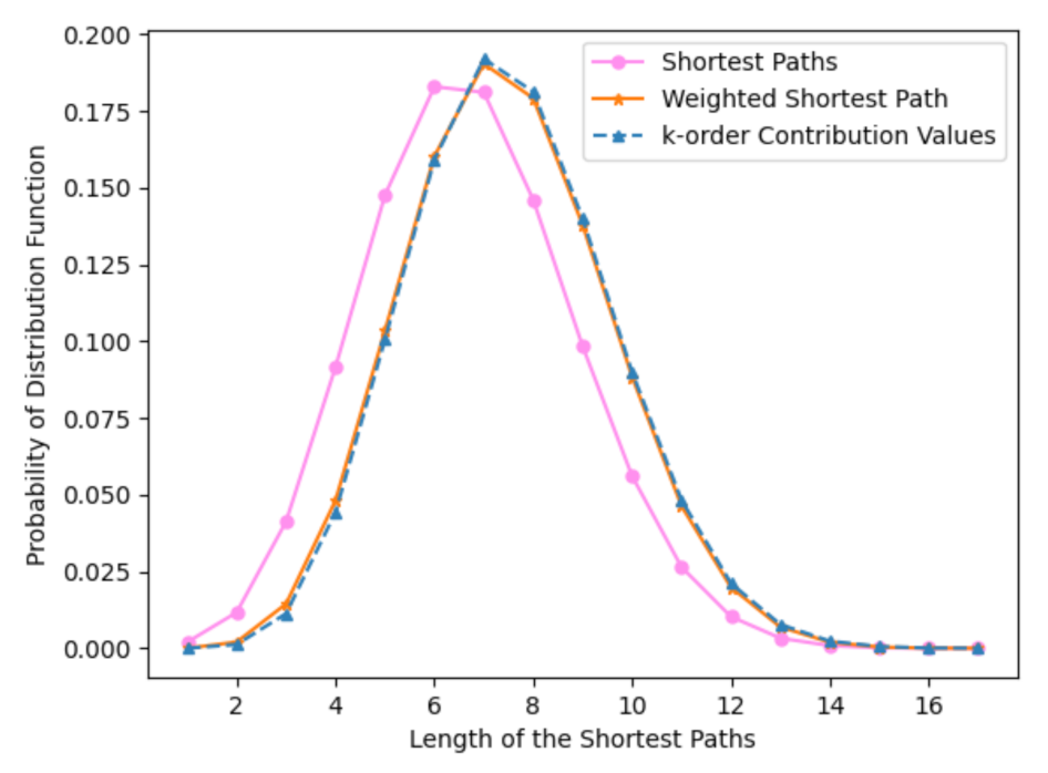
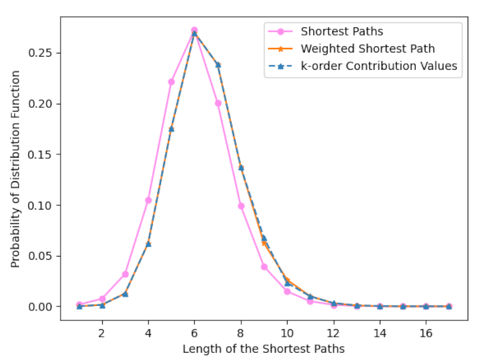
We discover the distribution of shortest paths has intrinsic correlation with the betweenness distribution, and experimental evidence confirms this relationship;
3.
We find that the betweenness centrality indices of some nodes are 0, but these nodes are not edge nodes and characterize critical significance in real networks.
In Section 2, we introduce the theoretical foundation of betweenness centrality and its typical algorithms. In Section 3, we elaborate the design of the NAHAN algorithm. In Section 4, we describe the intrinsic relationship with betweenness and the shortest paths distribution. In Section 5, we prove that some special nodes with betweenness centrality indices of 0 have critical significance in the network. In Section 6, we demonstrate that the distribution function of the shortest path and betweenness almost coincide. In Section 7, we conclude the work of this paper.

2. Related Work

In this section, we describe the related work of this paper in three aspects: the concept and properties of betweenness centrality, an introduction to Brandes’ algorithm, and an introduction to DAWN algorithm.

2.1. Betweenness Centrality

Bavelas et al. proposed betweenness centrality in an in-depth study of social networks [28]. Freeman described that the frequency of nodes’ occurrence on the shortest path directly affects their importance in the network, and proposed that evaluating the influence of nodes via betweenness centrality is rigorous [29,30]. Freeman expounded on the mathematical definition of betweenness centrality and the calculation method, which has complexities of O ( n 3 ) in time and O ( n 2 ) in space, where n is the number of nodes in the network.
Construct the connected network G = ( V , E ) , where V represents the set of nodes in the network, and E represents the set of edges. Betweenness centrality is usually divided into node betweenness centrality and edge betweenness centrality and has been defined as:    
B e t ( v ) = v i , v j V σ ( v i , v j v ) σ ( v i , v j ) , B e t ( e ) = v i , v j V σ ( v i , v j e ) σ ( v i , v j ) ,
where σ ( v i , v j ) represents the number of shortest paths passing between v i and v j , and σ ( v i , v j v ) and σ ( v i , v j e ) represents the number of shortest paths passing through v and e between v i and v j , respectively.

2.2. Brandes’ Algorithm

At present, Brandes’ algorithm is the best-known algorithm that exactly computes the betweenness centrality, which requires O ( m + n ) space and runs in O ( m n ) and O ( m n + n 2 l o g 2 n ) time on unweighted and weighted networks, respectively, where m is the number of links [4]. Erdős, Dóra et al. proposed its optimization [31,32,33]. Brandes’ algorithm has been integrated into a notable open-source project in the network analysis “NetworkX” [34].
Given the network G = ( V , E ) , the betweenness centrality of node v is defined as
B e t ( v ) = s t v V σ s t ( v ) σ s t = s t v V B e t s t ( v ) ,
and Brandes proposed the following formula to calculate betweenness centrality:
B e t s · ( v ) = w : v P s ( w ) σ s v σ s w [ 1 + B e t s · ( w ) ] ,
where B e t s · ( v ) represents the betweenness centrality of node v, which has the shortest path to other nodes, with node s being the source node in the network.

2.3. DAWN Algorithm

DAWN is a more efficient algorithm based on adjacency matrix operations for solving the all-source shortest paths problem, which requires O ( n 2 ) space and O ( d i m · n 2.387 ) time, where d i m is the diameter of the graph. DAWN can accelerate computing via a multi-GPU system, and its time complexity mainly depends on the number of nodes and is insensitive to the density of the graphs [27].
Feng et al. computed special matrix multiplications and vector multiplications to generate the number and length of shortest paths between all pairs of nodes, and adopted a dual matrix mode to store the calculation results: one for the shortest path lengths and another for the amount of the shortest paths with all pairs of nodes. The DAWN algorithm is expressed as follows on unweighted and weighted graphs:
A i j = 1 i n 1 j n a i j ( k ) , A i j w = 1 i n 1 j n a i j ( k ) + h i j ( k ) ,
where a i j ( k ) represents the number of shortest paths between nodes i and j, h i j ( k ) represents the number of weighted edges, k represents the length of the path between nodes i and j in the graph, and Formula (4) holds under the condition a i j ( k ) 0 i j 1 p k 1 a i j ( p ) = 0 .

3. Design of the NAHAN Algorithm

Classic complex network models mainly include the Erdős–Rényi random network model [35], Barabási–Albert scale-free network model [36,37,38], and Watts–Strogatz small-world network model [39,40]. In this section, we introduce the design of the NAHAN algorithm on the unweighted networks and weighted networks.

3.1. Unweighted Networks

The unweighted network G = ( V , E ) is conveniently described as an adjacency matrix:
A = a 11 a 1 n a n 1 a n n .
The entry a i j = 1 in adjacency matrix A means that there is an edge with a distance of 1 between node i and node j. We strip the edges connecting v to other nodes from the network, which means setting all the values in row i and column j to 0 in the adjacency matrix A to obtain a matrix B v . We define the iterative formulas of matrices A ( k ) , B v ( k ) and C v ( k ) as
A ( k + 1 ) = A ( k ) × A ( 1 ) , B v ( k + 1 ) = B v ( k ) × B v ( 1 ) , C v ( k + 1 ) = A ( k + 1 ) B v ( k + 1 ) ,
where the equation holds under condition 1 k < k + 1 n 1 . Although the definitions of the three matrices are similar, the slight gaps between them are the focus of the DAWN algorithm. We define them as follows:
1.
The element a i j ( k ) in matrix A ( k ) = a i j ( k ) represents the number of paths with the length k between nodes i and j in the network.
2.
The element b i j ( k ) in matrix B v ( k ) = b i j ( k ) represents the number of paths with the length k that do not pass through node v when going between nodes i and j in the network.
3.
The element c i j ( k ) in matrix C v ( k ) = c i j ( k ) represents the number of paths with the length k that pass through node v when going between nodes i and j in the network.
Given the above definitions of the matrices, we propose a new betweenness centrality calculation formula:
B e t A M ( v ) = 1 k n 1 1 i , j n i j F i j ( k | v ) .
We define F i j k as
F i j ( k | v ) = c i j ( k ) a i j ( k ) , a i j ( k ) 0 i j 1 p k 1 a i j ( p ) = 0 0 , Otherwise
where i j means not to calculate the circular path, which is consistent with the definition of betweenness described in Formula (2). 1 p k 1 a i j ( p ) = 0 represents that there is no path in the range [ 1 , k 1 ] , and a i j ( k ) 0 represents that there is the path from i to j. The paths that satisfy both conditions at the same time are the shortest paths from i to j. Formula (8) uses the matrix to describe Formula (2), which is the definition of betweenness.
The paths in the matrix F i j ( k | v ) are directed. The undirected edge can be represented by two directed edges, and the F i j ( k | v ) is a symmetric matrix on the undirected networks. To better analyze betweenness centrality, we suggest using the normalized Formula (9),
b e t A M ( v ) = 1 ( n 1 ) × ( n 2 ) 1 k n 1 1 i , j n i j F i j ( k | v ) .
We use pseudocode to describe the algorithm in Algorithm 1. We describe the mathematical foundation of the matrix and provide an example to facilitate the understanding of the algorithm in Appendix A and Appendix B.
Algorithm 1 Unweighted Networks
Input: A ( n ) , B ( n )
Output: b e t A M ( ν )
 1:
functionMAIN( A ( n ) , B ( n ) , b e t A M ( ν ) )
 2:
   b e t A M ( ν ) 0
 3:
  for  i = 1 n 2  do
 4:
    A ( i + 1 ) A ( i ) × A
 5:
    B ( i + 1 ) B ( i ) × B
 6:
    C ( i + 1 ) A ( i + 1 ) B ( i + 1 )
 7:
  end for
 8:
  for  k = 1 n  do
 9:
    s u m s u m + F ( k )
10:
  end for
11:
   b e t A M ( ν ) 1 ( n 1 ) × ( n 2 ) × s u m
12:
  return  b e t A M ( ν )
13: 
end function

3.2. Weighted Networks

The weighted network G = ( V , E , W ) is conveniently described as an adjacency matrix:
A w = w 11 w 1 n w n 1 w n n .
Let w be the weight indices of the edges. We assume that w N , where N is the set of natural numbers, and w i j represents the weight of the edge between nodes i and j.
First, we define matrices A w ( k ) , B v | w ( k ) , C v | w ( k ) and H A w ( k ) :
1.
Matrix A w ( k ) represents the number of paths with the weight k between nodes i and j in the network. Matrix A w ( 1 ) represents the adjacency matrix corresponding to the subnetwork formed by the edges with the weight 1 in the adjacency matrix A w .
2.
Matrix B v | w ( k ) represents the number of paths with weight k that do not pass through node v between nodes i and j in the network. Matrix B v | w ( 1 ) represents the adjacency matrix corresponding to the subnetwork formed by the edges with a weight of 1 that do not pass through node v in the adjacency matrix A w .
3.
Matrix C v | w ( k ) represents the number of paths with the weight k that pass through node v between nodes i and j in the network. Matrix C v | w ( k ) represents the adjacency matrix corresponding to the subnetwork formed by the edges with the weight 1 that pass through node v in the adjacency matrix A w .
4.
Matrix H A w ( k ) represents the adjacency matrix corresponding to the subnetwork formed by the edges with the weight k in the adjacency matrix A w . If there is no edge with the weight k in the network, then H A w ( k ) is a null matrix, and we also define H A w ( 1 ) as a null matrix.
Then, we define iterative formulas for matrix A w ( k ) as follows:
A w ( k + 1 ) = A w ( k ) × A w ( 1 ) + H A w ( k + 1 ) , 1 k < k + 1 w 0 A w ( k ) = A w ( r ) × A w ( λ w 0 ) , w 0 < k < n
where r = k mod w 0 , and λ = k r w 0 . Similar to matrix A w ( k ) , we define iterative formulas for matrix B w ( k ) as follows:
B v | w ( k + 1 ) = B v | w ( k ) × B v | w ( 1 ) + H B w ( k + 1 ) , 1 k < k + 1 w v B v | w ( k ) = B v | w ( r ) × B v | w ( λ w v ) , w v < k < n
where r = k mod w v , and λ = k r w v . H B w ( k ) represents the adjacency matrix corresponding to the subnetwork formed by the edges with the weight k in the adjacency matrix B v | w ( k ) , and H B w ( 1 ) is a null matrix. w 0 represents the upper limit of the weight of the weighted network represented by matrix A w ( k ) , and w v represents the upper limit of the weight of the weighted network represented by matrix B v | w ( k ) .
According to Formulas (11) and (12), we define the matrix C v | w ( k ) as
C v | w ( k ) = A w ( k ) B v | w ( k ) .
The calculation processes of the unweighted and weighted networks are the same except for the different matrix definitions and iterative formulas. Finally, we calculate the betweenness centrality of unweighted and weighted networks with Formula (7)–(9), respectively.

4. Distribution of Betweenness and Shortest Paths

Barabási–Albert scale-free networks and Erdős–Rényi random networks are the classic complex network models [35]. Betweenness centrality represents the frequency of nodes’ occurrence on the shortest path in the network. Previously, we studied the relationship of the betweenness and the average shortest path, which provided ideas for the research in this paper [41,42,43]. We obtain the following identity:
v V b e t ( v ) = l 1 , e E b e t ( e ) = l ,
where l represents the average shortest path of the networks.
The previous research proves the betweenness identities by exemplifying some special small-scale networks, due to being limited by the insufficiency of methods. In this section, we mathematically demonstrate the hierarchical correlation with betweenness and the distribution of shortest paths, which is an essential finding and makes the sum of betweenness equal to the shortest path average. We can calculate betweenness hierarchically by methodological advances and verify that correlation is ubiquitous and rigorous on real networks.
Katzav et al. studied the shortest paths distribution in the Erdős–Rényi network and proposed a distribution function [44]. Given the close connection between the shortest paths of betweenness centrality, we assume that there is a correlation between the distribution functions of the contribution value of betweenness centrality and the shortest paths on the general networks. First, we perform the sum operation on the definition of betweenness centrality:
v V B e t ( v ) = i j V { v } σ ( i , j | v ) σ ( i , j ) ,
and we obtain the derivation according to the formula (18):
v B e t ( v ) = v V F i j ( k | v ) = v V 1 i n 1 j n c i j ( k ) a i j ( k ) .
As the path length grows, the corresponding number of paths changes. To evaluate the effect of paths of different lengths on the betweenness distribution, we introduce the concept of k-order contribution value and use D B e t ( k | v ) to represent. We calculate the value within the current F matrix to obtain an intermediate value, and define this intermediate value as the k-order contribution values of betweenness centrality. The k-order contribution values represent the sum of the betweenness of all nodes under the condition that the length of shortest paths is k. We give the definition formula:
D B e t ( k | v ) = i j V { v } d i s t ( i , j ) = k σ ( i , j | v ) σ ( i , j ) ,
where D B e t ( k | v ) represents the k-order contribution values of node v, and d i s t ( i , j ) represents the length of the shortest paths between i and j. We notice that the function D B e t ( k | v ) is a piecewise function that is only related to k after summing all nodes in the networks:
D B e t ( k ) = v V D B e t ( k | v ) = v V i j V { v } d i s t ( i , j ) = k σ ( i , j | v ) σ ( i , j ) .
There are k + 1 nodes in the paths of length k, and the head and tail nodes of the paths are not included in the computations of betweenness centrality, which makes the number of nodes included in the calculation in each path k 1 . Based on the derivation, we simplify the above equation as
D B e t ( k ) = v V i j V { v } d i s t ( i , j ) = k σ ( i , j | v ) σ ( i , j ) = i j V { v } d i s t ( i , j ) = k d i s t ( i , j ) 1 .
We sum the shortest paths that exist between all pairs of nodes in the network:
D B e t ( k ) = i j V { v } d i s t ( i , j ) = k d i s t ( i , j ) 1 = ( k 1 ) f ( k ) ,
where f ( k ) represents the number of shortest paths of the length k.
This is a novel finding that reveals the correlation between the k-order contribution values of betweenness centrality and the shortest paths. We accumulate the k-order contribution values to reveal the relationship of betweenness centrality and average shortest paths:
v V b e t ( v ) = k = 1 d i m D b e t ( k ) = k = 1 d i m ( k 1 ) n 2 f ( k ) ,
where n 2 is the normalization coefficient. We construct the shortest path distribution function:
F s p ( k ) = f ( k ) k = 1 d i m f ( k ) = μ f ( k ) ,
where μ represents the constant coefficients of f ( k ) . We notice that there is a weighted relationship between the distribution functions of the shortest path and the k-order contribution values. We define the weighted shortest path distribution function as
F s p w ( k ) = ( k 1 ) f ( k ) k = 1 d i m ( k 1 ) f ( k ) = μ w ( k 1 ) f ( k ) ,
where μ w represents the constant coefficients of f ( k ) .
We have mathematically proved that there is a relationship between betweenness centrality and the shortest path distribution.

5. Betweenness Centrality of Special Nodes

Nodes with the betweenness centrality index 0 are ubiquitous in real networks. Researchers typically believe that these nodes appear at the edge of the networks. Combining the distribution of shortest paths, we find that such nodes appear even in the center of the networks. We propose three sufficient conditions for the betweenness centrality indices of nodes to be 0: Nodes have a degree of 1, specific nodes appear in the networks, and nodes appear within a specific connected component. It is generally accepted that the betweenness centrality indices of nodes with a degree of 1 are 0, and we discuss how to make up for the lack of single centrality by combined use of multiple centrality under special circumstances.

5.1. Specific Nodes in the Networks

Theorem 1.
There are specific nodes in undirected networks that form fully connected subgraphs with their first-order neighbor nodes, and the betweenness centrality indices of specific nodes are 0.
Proof of Theorem 1. 
We prove Theorem 1 in the following four steps:
1.
We assume that there is the node 1, which forms the undirected network G 1 with the first-order neighbor nodes 2, 3 ( G 1 is shown in Figure 1);
2.
There is a shortest path of length 1 between nodes 2 and 3, so the betweenness centrality index of node 1 is 0;
3.
Step 2 illustrates that Theorem 1 holds in Figure 1, and we add the node 3, which is potentially connected to any of three nodes;
  • When node 4 is connected to node 2 and 3, the betweenness centrality index of node 1 is 0;
  • When node 4 is connected to node 1, the shortest path from node 4 to node 2 and 3 passes through node 2, and the betweenness centrality index of node 2 is not 0;
  • It is necessary to add edges and nodes, which makes the betweenness centrality index of the node 1, and forms an undirected network ( G 2 ), which is shown in Figure 2);
  • The network shown in Figure 2 is a fully connected subgraph formed by node 1 and its first-order neighbor nodes.
4.
Arbitrary networks containing the special nodes can be formed by adding nodes and edges to the networks shown in Figure 1 and Figure 2.
In summary, we have proved Theorem 1. □
We have proved that Theorem 1 holds in arbitrary networks containing special nodes, and define the subgraph formed by nodes 1, 2, and 3, as the B 0 t r i a n g l e . The isolated nodes in the networks are the special B 0 t r i a n g l e , which forms a fully connected subgraph with itself. It is not guaranteed to find the B 0 t r i a n g l e in arbitrary networks, which is why Theorem 1 is irreversible, such as the star networks (shown in Figure 2).

5.2. Fully Connected Component

Theorem 2.
There are fully connected components in undirected networks, and the betweenness centrality indices of nodes in the connected component are 0 except for the nodes connected to the other component.
Proof of Theorem 2. 
We prove Theorem 2 in the following four steps:
1.
We assume that there is a specific connected component, which is a fully connected component and is represented by an undirected network ( G 3 ) (shown in Figure 3);
2.
Each pair of nodes in the connected component has the shortest paths of length 1, which makes the betweenness centrality indices of nodes 0;
3.
Step 2 illustrates that Theorem 2 is established in Figure 3; we add node v s to Figure 3, and it can reach arbitrary nodes under the condition that the shortest path length is 2;
4.
In the case of step 3, in the connected component, except for the nodes connected to the v s , the betweenness centrality indices of nodes is 0.
In summary, we have proved Theorem 2. □
We have proved that Theorem 2 holds on the fully connected components. Theorems 1 and 2 can be associated and verified with each other, but they describe different objects. Theorem 1 guarantees that the betweenness centrality of the special node under certain conditions is 0, and Theorem 2 describes the universal phenomenon that all nodes in fully connected components obey. In real networks, the nodes described by Theorems 1 and 2 usually behave as redundant backup paths and aggregated communities, respectively.

5.3. Contribution of Special Nodes

Theorem 3.
The arbitrary path that is the shortest path with a length greater than 2 and passing through node v contains a shortest path with the length 2 that passes through node v.
Theorem 3 can be proved by the definition of the shortest path, which will not be repeated here. The sum of the frequencies of all nodes appears on the shortest path in the hierarchical network, which we call the k-order contribution value, and the network is layered according to the shortest path length. We rigorously formulate the k-order contribution values using mathematical formulas in Section 4. Combining Theorem 3, we can obtain two corollaries:
1.
For the nodes for which betweenness centrality is not 0, there is at least one shortest path of length 2 passing through the node;
2.
The betweenness centrality indices of the node with a second-order contribution value of 0 must be 0.
We propose a mathematical foundation that supports the optimization of the NAHAN algorithm. The nodes with the second-order contribution value of 0 do not need to continue the operation, which reduces the computation time. The optimization does not affect the accuracy and is only related to the structure of the networks. When the network is extremely sparse, there may be nodes with a degree of almost 1. In the study of real networks, some fully connected components also appear when they are relatively sparse. These nodes can be quickly searched by computing the 2-order betweenness contribution values via the NAHAN algorithm without having to compute the betweenness centrality of the entire network.

5.4. Discussion of Centrality Measures

Each centrality measure has its focus, and it is difficult to fully evaluate the importance of nodes with the single centrality measure. For example, the shortest path may not be selected in a routing network, since the processing power and line bandwidth of the router are limited. It is impossible to rigorously evaluate the importance of all nodes in the real networks through the single centrality measure. In order to evaluate the importance of the node, we need to choose the centrality measures according to the requirements in the scenarios. The importance of nodes can be objectively evaluated by using a combination of multiple centrality measures which considers the effects from multiple aspects.
Centrality measures are mainly defined based on the node neighbors, the paths, the eigenvectors, and the node set shrinkage, such as degree centrality measure [30], Katz centrality measure [45], eigenvector centrality measure [46], and residual closeness centrality measure [47]. The Katz centrality measure considers not only the shortest path between node pairs, but also other non-shortest paths between them, and assigns weights to the paths of different lengths. The Katz centrality measure takes into account the impact of other paths on node importance, and requires O ( n 3 ) time [48].
The importance of the special nodes we found can be correctly evaluated by using the eigenvector centrality measure and PageRank [49]. We can use the degree centrality measure to correctly evaluate the importance of nodes in the special subgraphs. Nodes in the special subgraphs have the same importance, except for nodes connected to other nodes out of the subgraph. The degree centrality measure can also effectively evaluate the importance of nodes in the global network. The number of links between nodes in the subgraph is fixed, which means that the number of links to nodes outside the subgraph determines the importance of the node.

6. Experimental Results

We verify the fit of the two distribution functions on the Erdős–Rényi networks, the Barabási–Albert networks, and the real networks. The Erdős–Rényi and Barabási–Albert network models were generated by NetworkX, which is widely used for the study of the complex networks [34]. The real network was derived from the Stanford University public dataset, which is a collaboration network covering scientific collaborations between authors of papers submitted to the general relativity and quantum cosmology categories on the e-print arXiv [50].
In order to intuitively reflect the relationship between the contribution value and the shortest path distribution, we normalized them as
F s p ( k ) = f ( k ) k = 1 d i m f ( k ) ,
F s p w ( k ) = ( k 1 ) f ( k ) k = 1 d i m ( k 1 ) f ( k ) ,
F d ( k ) = D b e t ( k ) k = 1 d i m D b e t ( k ) ,
and we plotted the shortest path distribution, the weighted shortest path distribution, and the k-order contribution value distribution curve. We used NetworkX to generate an Erdős–Rényi network with 1000 nodes and the connection probability of 0.004; the results are shown in Figure 4.
For the Erdős–Rényi networks, the weighted shortest path distribution and the k-order contribution values distribution line almost completely coincided, showing a good degree of fit. We tested the fitting performance of the k-order contribution value distribution function on the Barabási–Albert network, and used NetworkX to generate a Barabási–Albert network with 1000 nodes and one edge to attach from a new node to existing nodes. The results are shown in Figure 5.
Figure 4 and Figure 5 show that there was a good fit between the distribution functions on the network model generated by calculations. The real networks were not strictly Barabási–Albert networks and Erdős–Rényi networks, so we tested the fit of the distribution function on the real network to verify the generality of predicting the distribution of shortest paths in the network via the k-order contribution values. The results are shown in Figure 6.
We studied the special nodes and connected components that exist in routing networks. A typical example of a special node is a backup route, whose main role is to balance network traffic and improve network survivability. A typical example of a special connected branch is the core of a routing network, consisting of multiple interconnected routers. The routes that are not connected to the outside are mainly responsible for balancing the load of the core network. Even nodes with 0 betweenness centrality may play an important role in the network, and evaluating node importance by a single index may no longer be suitable for increasingly complex networks.

7. Conclusions

In this paper, we propose an algorithm for hierarchical analysis networks, enabling us to study betweenness centrality in depth. We discover that the distribution of shortest path has intrinsic correlation with the betweenness distribution, and verify the fact both on the generated networks and real networks. The intrinsic correlation shows that the shortest paths with various lengths have different effects on the betweenness centrality. Furthermore, we identify that there are some special nodes with betweenness centrality indices of 0 which are not edge nodes. Even nodes with 0 betweenness centrality may play an important role in the real networks, such as backup routes and fixed academic teams. Thus, evaluating node importance by the single centrality measure may no longer be suitable for increasingly complex networks. We discuss that the combination of centrality measures to evaluate the importance of nodes would be more objective and rigorous.

Author Contributions

Validation, C.C.; Writing—original draft, Y.F.; Writing—review & editing, H.W. and H.L. All authors have read and agreed to the published version of the manuscript.

Funding

This research is partially supported by the National Natural Science Foundation of China under Grant No. 62002377.

Data Availability Statement

Data used in this paper were generated by NetworkX, which is widely used for the study of the complex networks. The real network was derived from the Stanford University public dataset, which can be found in http://snap.stanford.edu/data/ca-GrQc.html (accessed on 23 June 2022). The code of this paper can be found in https://github.com/lxrzlyr/Betweenness-centrality.git (accessed on 23 June 2022).

Conflicts of Interest

The authors declare no conflict of interest.

Abbreviations

The following abbreviations are used in this manuscript:
NotationDefinition
GA graph
V , E , W Set of nodes, edges and weights
v , e , w A node, edge and weight of edges
B e t , b e t Betweenness centrality and its normalization
A , A w Adjacency matrix of unweighted graphs and weighted graphs
B v , B v | w Adjacency matrix of unweighted graphs and weighted graphs without v
C v , C v | w Adjacency matrix of unweighted graphs and weighted graphs through v
F i j ( k | v ) Occurrence frequency of node v with the shortest paths length k
D B e t ( k | v ) K-order contribution value of node v with the shortest paths length k
μ Constant parameter

Appendix A. Example

This is a undirected and unweighted graph G = ( V , E ) with 8 nodes and 13 edges.
Figure A1. Example figure of undirected and unweighted graph G = ( V , E ) with 8 nodes and 13 edges. The diameter of the graph is 3.
Mathematics 10 02521 g0a1
We denote its adjacency matrix as:
A = 0 1 0 1 0 0 1 1 1 0 1 0 0 1 0 0 0 1 0 1 1 0 0 0 1 0 1 0 1 0 0 0 0 0 1 1 0 1 0 1 0 1 0 0 1 0 1 0 1 0 0 0 0 1 0 1 1 0 0 0 1 0 1 0 .
We exemplify the matrices A ( k ) , B 1 ( k ) , C 1 ( k ) and F ( k | 1 ) of this graph. The range of k is [ 1 , 3 ] , because the diameter of the graph is 3.
A ( 1 ) = 0 1 0 1 0 0 1 1 1 0 1 0 0 1 0 0 0 1 0 1 1 0 0 0 1 0 1 0 1 0 0 0 0 0 1 1 0 1 0 1 0 1 0 0 1 0 1 0 1 0 0 0 0 1 0 1 1 0 0 0 1 0 1 0 , B 1 ( 1 ) = 0 0 0 0 0 0 0 0 0 0 1 0 0 1 0 0 0 1 0 1 1 0 0 0 0 0 1 0 1 0 0 0 0 0 1 1 0 1 0 1 0 1 0 0 1 0 1 0 0 0 0 0 0 1 0 1 0 0 0 0 1 0 1 0 ,
A ( 2 ) = 4 0 2 0 2 2 1 1 0 3 0 2 2 0 2 1 2 0 3 1 1 2 0 1 0 2 1 3 1 1 1 2 2 2 1 1 4 0 2 0 2 0 2 1 0 3 0 2 1 2 0 1 2 0 3 1 1 1 1 2 0 2 1 3 , B 1 ( 2 ) = 0 0 0 0 0 0 0 0 0 3 0 2 2 0 2 1 0 0 3 1 1 2 0 1 0 2 1 3 1 1 1 2 0 2 1 1 4 0 2 0 0 0 2 1 0 3 0 2 0 2 0 1 2 0 3 1 0 1 1 2 0 2 1 3 ,
A ( 3 ) = 2 8 2 8 5 3 7 7 8 0 7 2 3 7 1 4 2 7 2 6 7 1 5 3 8 2 6 2 7 4 3 2 5 3 7 7 2 8 2 8 3 7 1 4 8 0 7 2 7 1 5 3 2 7 2 6 7 4 3 2 8 2 6 2 , B 1 ( 3 ) = 0 0 0 0 0 0 0 0 0 0 7 2 3 7 1 4 0 7 2 6 7 1 5 3 0 2 6 2 7 4 3 2 0 3 7 7 2 8 2 8 0 7 1 4 8 0 7 2 0 1 5 3 2 7 2 6 0 4 3 2 8 2 6 2 .
We exemplify the matrices C 1 ( k ) and F ( k | 1 ) as follows. “#” represents that the value of this position is not included in the calculation of the betweenness centrality indices. “*” represents that the value is to be calculated, and if the value does not appear, it will finally be recorded as 0. F ( k | 1 ) corresponds to the operations of betweenness centrality for node 0 in the networks. The values in row 0 and column 0 are not included in the calculations. We do not consider the situation in which the path starts and ends overlap in calculating the shortest path, so we exclude the case of i = j .
C 1 ( 1 ) = 0 1 0 1 0 0 1 1 1 0 0 0 0 0 0 0 0 0 0 0 0 0 0 0 1 0 0 0 0 0 0 0 0 0 0 0 0 0 0 0 0 0 0 0 0 0 0 0 1 0 0 0 0 0 0 0 1 0 0 0 0 0 0 0 , F ( 1 | 1 ) = # # # # # # # # # # 0 0 # 0 # 0 0 # 0 # 0 # 0 0 # 0 0 # 0 0 # 0 # 0 # 0 # 0 0 # ,
C 1 ( 2 ) = 4 0 2 0 2 2 1 1 0 1 0 1 0 0 1 1 2 0 0 0 0 0 0 0 0 1 0 1 0 0 1 1 2 0 0 0 0 0 0 0 2 0 0 0 0 0 0 0 1 1 0 1 0 0 1 1 1 1 0 1 0 0 1 1 , F ( 2 | 1 ) = # # # # # # # # # # 0 0.5 0 0 0.5 1 # 0 # 0 0 0 0 # 0.5 0 # 0 0 1 0.5 # 0 0 0 # 0 0 0 # 0 0 0 0 # 0 0 # 0.5 1 0 0 # 0 # 1 0 0.5 0 0 0 # ,
C 1 ( 3 ) = 2 8 2 8 5 3 7 7 8 0 2 0 2 2 1 1 2 2 0 2 0 0 2 2 8 0 2 0 2 2 1 1 5 2 0 2 0 0 2 2 3 2 0 2 0 0 2 2 7 1 2 1 2 2 2 2 7 1 2 1 2 2 2 2 , F ( 3 | 1 ) = # # # # # # # # # # 0 0.5 0 0 0.5 1 # 0 # 0 0 0 0.4 0 # 0.5 0 # 0 0 1 0.5 # 0 0 0 # 0 0 0 # 0 0 0 0 # 0 0 # 0.5 0.4 1 0 0 # 0 # 1 0 0.5 0 0 0 # .
The betweenness centrality of node 0 is 0.18571428571428572 , and it can be verified by the Brandes’ algorithm.

Appendix B. Mathematical Foundation

The unweighted network G = ( V , E ) is conveniently described as an adjacency matrix:
A = a 11 a 1 n a n 1 a n n .
The adjacency matrix is a square matrix which represent the graphs, in which the entry a i j = 1 if path between node i and j is in the graph, while a i j = 0 if path between node i and j is not in the graph [51].
Theorem A1.
The element a i j ( k ) in matrix A ( k ) = a i j ( k ) represents the number of paths with the length k between nodes i and j in the network.
Proof. 
We use the cumulative formula to express the multiplication of matrices:
C = A × B = c i j n × n ,
Thus, c i j is obtained from the ith row of A and the jth column of B.
c i j = a i 1 b 1 j + a i 2 b 2 j + a i n b n j = k = 1 n a i k b k j ,
Matrix multiplication and its applicability to graphs are illustrated in Appendix A. The adjacency matrix A of the graph is shown together with its powers A 2 and A 3 . Some of the entries of A 2 will now be worked out in detail:
a 12 ( 2 ) = a 11 a 12 + a 12 a 22 + a 13 a 32 + a 14 a 42 + a 15 a 52 + a 16 a 62 + a 17 a 72 + a 18 a 82 = 0 · 1 + 1 · 0 + 0 · 1 + 1 · 0 + 0 · 0 + 0 · 1 + 1 · 0 + 1 · 0 , = 0 ,
Together these lines form a number of length 2 from 1 to 2, which in this case is not a existing path. The fact that there is in the G exactly no path of length 2 from 1 to 2 is reflected in the value a 12 ( 2 ) = 0 . □
In summary, we have proved the above Theorem A1, which is the mathematical foundation of the algorithm.

References

  1. Li, D.; Ma, J.; Yao, C.; Chen, W.; Zhang, Z. Informatization Promotes Accurate Management and Open Sharing of National Natural Science Fund. In China’s e-Science Blue Book 2018; Springer: Singapore, 2020; pp. 219–234. [Google Scholar]
  2. Tizghadam, A.; Leon-Garcia, A. Betweenness centrality and resistance distance in communication networks. IEEE Netw. 2010, 24, 10–16. [Google Scholar] [CrossRef]
  3. Puzis, R.; Altshuler, Y.; Elovici, Y.; Bekhor, S.; Shiftan, Y.; Pentland, A. Augmented betweenness centrality for environmentally aware traffic monitoring in transportation networks. J. Intell. Transp. Syst. 2013, 17, 91–105. [Google Scholar] [CrossRef] [Green Version]
  4. Brandes, U. A faster algorithm for betweenness centrality. J. Math. Sociol. 2001, 25, 163–177. [Google Scholar] [CrossRef]
  5. Jin, S.; Huang, Z.; Chen, Y.; Chavarría-Miranda, D.; Feo, J.; Wong, P.C. A novel application of parallel betweenness centrality to power grid contingency analysis. In Proceedings of the 2010 IEEE International Symposium on Parallel and Distributed Processing (IPDPS), Atlanta, GA, USA, 19–23 April 2010; pp. 1–7. [Google Scholar]
  6. Mehmood, A.; Choi, G.S.; von Feigenblatt, O.F.; Park, H.W. Proving ground for social network analysis in the emerging research area “Internet of Things”(IoT). Scientometrics 2016, 109, 185–201. [Google Scholar] [CrossRef]
  7. Zhou, T.; Bo, W.; Wang, B. Overview of complex network research. Physics 2005, 34. [Google Scholar]
  8. Guo, L.; Xu, X. Complex Networks; Shanghai Science and Technology Education Press: Shanghai, China, 2010; pp. 1–15. [Google Scholar]
  9. Barabási, A.L. Network science. Philos. Trans. R. Soc. A Math. Phys. Eng. Sci. 2013, 371, 7–9. [Google Scholar] [CrossRef]
  10. González, H.F.; Narasimhan, S.; Johnson, G.W.; Wills, K.E.; Haas, K.F.; Konrad, P.E.; Chang, C.; Morgan, V.L.; Rubinov, M.; Englot, D.J. Role of the nucleus basalis as a key network node in temporal lobe epilepsy. Neurology 2021, 96, e1334–e1346. [Google Scholar] [CrossRef] [PubMed]
  11. Stoffers, D.; Altena, E.; van der Werf, Y.D.; Sanz-Arigita, E.J.; Voorn, T.A.; Astill, R.G.; Strijers, R.L.; Waterman, D.; Van Someren, E.J. The caudate: A key node in the neuronal network imbalance of insomnia? Brain 2014, 137, 610–620. [Google Scholar] [CrossRef] [PubMed] [Green Version]
  12. Pereira, J.; Saura, S.; Jordan, F. Single-node vs. multi-node centrality in landscape graph analysis: Key habitat patches and their protection for 20 bird species in NE Spain. Methods Ecol. Evol. 2017, 8, 1458–1467. [Google Scholar] [CrossRef]
  13. Liu, F.; Xiao, B.; Li, H. Finding key node sets in complex networks based on improved discrete fireworks algorithm. J. Syst. Sci. Complex. 2021, 34, 1014–1027. [Google Scholar] [CrossRef]
  14. Ding, J.; Wen, C.; Li, G. Key node selection in minimum-cost control of complex networks. Phys. A Stat. Mech. Appl. 2017, 486, 251–261. [Google Scholar] [CrossRef]
  15. Li, X.; Tang, Y.; Du, Y.; Li, Y. Key Node Discovery Algorithm Based on Multiple Relationships and Multiple Features in Social Networks. Math. Probl. Eng. 2021, 2021, 1956356. [Google Scholar] [CrossRef]
  16. Gómez, D.; Castro, J.; Gutiérrez, I.; Espínola, R. A New Edge Betweenness Measure Using a Game Theoretical Approach: An Application to Hierarchical Community Detection. Mathematics 2021, 9, 2666. [Google Scholar] [CrossRef]
  17. Grobelny, B.T.; London, D.; Hill, T.C.; North, E.; Dugan, P.; Doyle, W.K. Betweenness centrality of intracranial electroencephalography networks and surgical epilepsy outcome. Clin. Neurophysiol. 2018, 129, 1804–1812. [Google Scholar] [CrossRef]
  18. Makarov, V.V.; Zhuravlev, M.O.; Runnova, A.E.; Protasov, P.; Maksimenko, V.A.; Frolov, N.S.; Pisarchik, A.N.; Hramov, A.E. Betweenness centrality in multiplex brain network during mental task evaluation. Phys. Rev. E 2018, 98, 062413. [Google Scholar] [CrossRef]
  19. Arasteh, M.; Alizadeh, S. A fast divisive community detection algorithm based on edge degree betweenness centrality. Appl. Intell. 2019, 49, 689–702. [Google Scholar] [CrossRef]
  20. Nigam, R.; Sharma, D.K.; Jain, S.; Srivastava, G. A local betweenness centrality based forwarding technique for social opportunistic IoT networks. Mob. Netw. Appl. 2022, 27, 547–562. [Google Scholar] [CrossRef]
  21. Tokito, S.; Kagawa, S.; Hanaka, T. Hypothetical extraction, betweenness centrality, and supply chain complexity. Econ. Syst. Res. 2022, 34, 111–128. [Google Scholar] [CrossRef]
  22. Liu, W.; Li, X.; Liu, T.; Liu, B. Approximating betweenness centrality to identify key nodes in a weighted urban complex transportation network. J. Adv. Transp. 2019, 2019, 9024745. [Google Scholar] [CrossRef]
  23. Xing, L.; Dong, X.; Guan, J.; Qiao, X. Betweenness centrality for similarity-weight network and its application to measuring industrial sectors’ pivotability on the global value chain. Phys. A Stat. Mech. Appl. 2019, 516, 19–36. [Google Scholar] [CrossRef]
  24. Madduri, K.; Ediger, D.; Jiang, K.; Bader, D.A.; Chavarria-Miranda, D. A faster parallel algorithm and efficient multithreaded implementations for evaluating betweenness centrality on massive datasets. In Proceedings of the 2009 IEEE International Symposium on Parallel & Distributed Processing, Rome, Italy, 23–29 May 2009; pp. 1–8. [Google Scholar]
  25. Bader, D.A.; Kintali, S.; Madduri, K.; Mihail, M. Approximating betweenness centrality. In International Workshop on Algorithms and Models for the Web-Graph; Springer: Berlin/Heidelberg, Germany, 2007; pp. 124–137. [Google Scholar]
  26. Furno, A.; El Faouzi, N.E.; Sharma, R.; Zimeo, E. Fast approximated betweenness centrality of directed and weighted graphs. In Complex Networks and Their Applications; Springer: Cham, Switzerland, 2018; pp. 52–65. [Google Scholar]
  27. Feng, Y.; Wang, H.; Lu, H. A Faster Algorithm for Betweenness Centrality Based on Adjacency Matrices. arXiv 2022, arXiv:2205.00162. [Google Scholar]
  28. Bavelas, A. Communication patterns in task-oriented groups. J. Acoust. Soc. Am. 1950, 22, 725–730. [Google Scholar] [CrossRef]
  29. Freeman, L.C. A set of measures of centrality based on betweenness. Sociometry 1977, 40, 35–41. [Google Scholar] [CrossRef]
  30. Freeman, L.C. Centrality in social networks conceptual clarification. Soc. Netw. 1978, 1, 215–239. [Google Scholar] [CrossRef] [Green Version]
  31. Wang, W.; Tang, C.Y. Distributed computation of node and edge betweenness on tree graphs. In Proceedings of the 52nd IEEE Conference on Decision and Control, Firenze, Italy, 10–13 December 2013; pp. 43–48. [Google Scholar]
  32. Erdős, D.; Ishakian, V.; Bestavros, A.; Terzi, E. A divide-and-conquer algorithm for betweenness centrality. In Proceedings of the 2015 SIAM International Conference on Data Mining, Vancouver, BC, Canada, 30 April–2 May 2015; pp. 433–441. [Google Scholar]
  33. Bentert, M.; Dittmann, A.; Kellerhals, L.; Nichterlein, A.; Niedermeier, R. An Adaptive Version of Brandes’ Algorithm for Betweenness Centrality. arXiv 2018, arXiv:1802.06701. [Google Scholar] [CrossRef]
  34. Hagberg, A.; Swart, P.; Chult, D.S. Exploring Network Structure, Dynamics, and Function Using NetworkX; Technical Report; Los Alamos National Lab. (LANL): Los Alamos, NM USA, 2008. [Google Scholar]
  35. Erdős, P.; Rényi, A. On the evolution of random graphs. Publ. Math. Inst. Hung. Acad. Sci 1960, 5, 17–60. [Google Scholar]
  36. Barabási, A.L.; Albert, R. Emergence of scaling in random networks. Science 1999, 286, 509–512. [Google Scholar] [CrossRef] [Green Version]
  37. Albert, R.; Jeong, H.; Barabási, A.L. Diameter of the world-wide web. Nature 1999, 401, 130–131. [Google Scholar] [CrossRef] [Green Version]
  38. Faloutsos, M.; Faloutsos, P.; Faloutsos, C. On power-law relationships of the internet topology. ACM SIGCOMM Comput. Commun. Rev. 1999, 29, 251–262. [Google Scholar] [CrossRef]
  39. Watts, D.J.; Strogatz, S.H. Collective dynamics of ‘small-world’networks. Nature 1998, 393, 440–442. [Google Scholar] [CrossRef]
  40. Amaral, L.A.N.; Scala, A.; Barthelemy, M.; Stanley, H.E. Classes of small-world networks. Proc. Natl. Acad. Sci. USA 2000, 97, 11149–11152. [Google Scholar] [CrossRef] [PubMed] [Green Version]
  41. Wang, H.; Wang, C.; Shu, N.; Ma, C.; Yang, F. The Betweenness Identities and Their Applications. In Proceedings of the 2020 IEEE 20th International Conference on Communication Technology (ICCT), Nanning, China, 28–31 October 2020; pp. 1065–1069. [Google Scholar] [CrossRef]
  42. Shu, N.; Wang, H.; Wang, C.; Zhu, X.; Ma, C.; Chang, C. Global Betweenness Identities in the Networks. In Proceedings of the 2021 IEEE 21st International Conference on Communication Technology (ICCT), Tianjin, China, 13–16 October 2021; pp. 783–786. [Google Scholar] [CrossRef]
  43. Wang, H.; Ma, T.; Wang, C.; Shu, N.; Huang, J.; Wang, M. The Bridge and Link Betweenness in the Networks. In Proceedings of the 2020 IEEE 20th International Conference on Communication Technology (ICCT), Nanning, China, 28–31 October 2020; pp. 1097–1101. [Google Scholar] [CrossRef]
  44. Katzav, E.; Nitzan, M.; Ben-Avraham, D.; Krapivsky, P.; Kühn, R.; Ross, N.; Biham, O. Analytical results for the distribution of shortest path lengths in random networks. EPL (Europhys. Lett.) 2015, 111, 26006. [Google Scholar] [CrossRef] [Green Version]
  45. Katz, L. A new status index derived from sociometric analysis. Psychometrika 1953, 18, 39–43. [Google Scholar] [CrossRef]
  46. Bonacich, P. Factoring and weighting approaches to status scores and clique identification. J. Math. Sociol. 1972, 2, 113–120. [Google Scholar] [CrossRef]
  47. Dangalchev, C. Residual closeness in networks. Phys. A Stat. Mech. Appl. 2006, 365, 556–564. [Google Scholar] [CrossRef]
  48. Liao, H.; Mariani, M.S.; Medo, M.; Zhang, Y.C.; Zhou, M.Y. Ranking in evolving complex networks. Phys. Rep. 2017, 689, 1–54. [Google Scholar] [CrossRef] [Green Version]
  49. Brin, S.; Page, L. The anatomy of a large-scale hypertextual web search engine. Comput. Netw. ISDN Syst. 1998, 30, 107–117. [Google Scholar] [CrossRef]
  50. Leskovec, J.; Kleinberg, J.; Faloutsos, C. Graph evolution: Densification and shrinking diameters. ACM Trans. Knowl. Discov. Data (TKDD) 2007, 1, 2-es. [Google Scholar] [CrossRef]
  51. Harary, F.; Norman, R.Z.; Cartwright, D. Structural Models: An Introduction to the Theory of Directed Graphs; Wiley: New York, NY, USA, 1965; Volume 5, pp. 111–115. [Google Scholar]
Figure 1. Example Networks with Specific Nodes. (a) is composed of nodes 1, 2 and 3, and (b) is composed of nodes 1,2,3, and 4. Example networks are composed of a specific node (1) and its first-order neighbor nodes, which form fully connected subgraphs. (a) Undirected Network G 1 ; (b) Undirected Network G 2 .
Mathematics 10 02521 g001
Figure 2. The star-sharp network proves that the inverse propositions of Theorems 1 and 2 do not hold. The star-sharp network consists of 17 nodes and 16 edges.
Mathematics 10 02521 g002
Figure 3. Example Networks as Specific Connected Components. Example networks are composed of fully connected components with 8 nodes and 28 edges.
Mathematics 10 02521 g003
Figure 4. The distribution of weighted shortest path and the k-order contribution value in the Erdős–Rényi network with 1000 nodes and the connection probability of 0.004.
Mathematics 10 02521 g004
Figure 5. The distribution of weighted shortest path and the k-order contribution value in the Barabási–Albert network with 1000 nodes and one edge to attach from a new node to existing nodes.
Mathematics 10 02521 g005
Figure 6. The distribution of weighted shortest path and the k-order contribution value on the real network with 5242 nodes and 14,496 edges, which is a collaboration network covering scientific collaborations between authors of papers submitted to general relativity and quantum cosmology categories on the e-print arXiv.
Mathematics 10 02521 g006
Publisher’s Note: MDPI stays neutral with regard to jurisdictional claims in published maps and institutional affiliations.

