
Benchmarking Cost-Effective Opinion Injection Strategies in Complex Networks

Department of Computer and Information Technology, Politehnica University Timişoara, 300006 Timişoara, Romania
Mathematics 2022, 10(12), 2067; https://doi.org/10.3390/math10122067
Submission received: 17 May 2022
/
Revised: 9 June 2022
/
Accepted: 13 June 2022
/
Published: 15 June 2022
(This article belongs to the Special Issue Complex Network Modeling: Theory and Applications)
Abstract
:Inferring the diffusion mechanisms in complex networks is of outstanding interest since it enables better prediction and control over information dissemination, rumors, innovation, and even infectious outbreaks. Designing strategies for influence maximization in real-world networks is an ongoing scientific challenge. Current approaches commonly imply an optimal selection of spreaders used to diffuse and indoctrinate neighboring peers, often overlooking realistic limitations of time, space, and budget. Thus, finding trade-offs between a minimal number of influential nodes and maximizing opinion coverage is a relevant scientific problem. Therefore, we study the relationship between specific parameters that influence the effectiveness of opinion diffusion, such as the underlying topology, the number of active spreaders, the periodicity of spreader activity, and the injection strategy. We introduce an original benchmarking methodology by integrating time and cost into an augmented linear threshold model and measure indoctrination expense as a trade-off between the cost of maintaining spreaders’ active and real-time opinion coverage. Simulations show that indoctrination expense increases polynomially with the number of spreaders and linearly with the activity periodicity. In addition, keeping spreaders continuously active instead of periodically activating them can increase expenses by 69–84% in our simulation scenarios. Lastly, we outline a set of general rules for cost-effective opinion injection strategies.
Keywords:
network science; opinion dynamics; influence maximization; cost-effectiveness; opinion injection strategies; networked controlMSC:
05C82; 91D30; 37M10; 93B701. Introduction
Understanding the dynamics of influence, which shape many aspects of our social life, is one of the main driving forces in network science [1,2]. A widely adopted approach to exploring temporal dynamics in networks—such as the way intricate relationships between individuals evolve over time—consists of identifying the most powerful or influential spreaders corroborated with centrality analysis and community detection [3,4,5,6]. However, pinpointing influential nodes in real-world networks is a considerable ongoing challenge relevant in interdisciplinary applications, such as information propagation, controlling rumors and disease outbreaks, designing recommender systems, and understanding the organization of social and ecological networks [1,3,7,8,9,10].
The idea of maximizing influence in networks is not new [5,11,12,13,14], but research on combining the maximization of influence coverage with the minimization of the cost of operation is limited. To address this issue, we propose investigating the trade-off between the cost of maintaining active spreaders and the spreading coverage to minimize what we call the indoctrination expense over a given complex network. Thus, our research aims to answer the following questions:
- How does the number of spreader agents scale with the indoctrination expense?
- How does the network topology influence the spreading effectiveness?
- How does the duration of spreader activity influence the trade-off between cost per agent and diffusion coverage?
- How does periodicity in spreader activity (i.e, periods of activity, followed by periods of inactivity) scale with costs and long-term indoctrination?
Answering these questions should lead us toward developing a set of “rules of thumb” for cost-effective spreading of opinion, information, or influence in social networks with a direct impact in interdisciplinary applications, such as viral marketing, sociology, and business applications.
We start from the premise that targeted diffusion of opinion in real-world contexts regularly incurs a cost for keeping spreader agents active, e.g., financial support toward marketing agents, political activists, or technological evangelists. However, studies on influence maximization (IM) originating from complex network theory typically ignore the underlying financial aspects [5,11,12]. Similarly, studies in the social sciences generally omit the network modeling paradigm [15,16]. Moreover, the impact of timing in the estimation of cost of operation is evident and has yet to be well explored in network science.
We find few temporal aspects corroborated to the opinion diffusion cost discussed in the state of the art. For example, in [17], Aral et al. introduce a distinction between the concepts of contagion (fast short-term influence) and homophily (slow long-term influence), and the authors show that homophily can explain more than 50% of contagion (influence). Furthermore, we find two studies on the temporal dynamics of diffusion [18,19] in which time is taken into account in the equation of opinion transmission and opinion survival that focus more on reproducing opinion cascades as they occurred in time.
Therefore, the driving motivation of this paper is to study the impact of key network parameters—such as the number of spreaders, nature of topology, number of opinions, spreader activity periodicity, and spreader activity duration—on diffusion effectiveness from the point of view of cost of operation. To the best of our knowledge, the described methodology and the insights obtained are a scientific novelty.
Taken together, our main contribution represents the original benchmarking methodology of adapting a classic linear threshold model [20,21] with time and cost characteristics, which is further used to measure opinion diffusion cost-effectiveness on a variety of synthetic and real-world complex network topologies via discrete event simulation. As a result, we highlight the common and distinct patterns that stimulate higher indoctrination expense based on key network characteristics.
The rest of the paper is structured in the following order: the Materials and Methods section presents the opinion diffusion model used for simulation, the temporal characteristics and the used network datasets; the Results section summarizes the simulation output and details the analysis over each experiment; the Discussion section presents a meta-analysis to understand the impact of each network parameter in isolation and draws conclusions from the experiments; the Conclusions outline the main results and enumerate the contributions of this work as well as possible future directions for research.
2. Materials and Methods
It is challenging to predict dynamic behavior at the meta-level of a network, even if we know how individual nodes respond to stimuli and how they are linked. Network science offers several notable graph-based predictive diffusion models [22], such as the classic linear threshold LT [20,21], the independent cascade IC [23], the classic voter model [24], the Axelrod model [25] and the Sznajd model [26]. These models use fixed thresholds to trigger opinion changes or thresholds that evolve according to simple probabilistic processes that are not driven by the internal state of social agents [22]. Other approaches may involve evolutionary game theory [27,28] to better model some aspects of social unpredictability. Also, it should be noted that we observe that the tolerance model [29,30] uses a dynamic threshold so that the states of the nodes evolve according to their interaction patterns.
Given the multitude of simulation parameters that we set out to analyze in this study, we consider incorporating a simple and proven diffusion model. Specifically, to achieve our research goals, we augment a classical linear threshold (LT) model [20,21] with cost constraints and implement discrete event computer simulation on several network models. Discrete event simulation is a recognized option in the network science literature for modeling high complexity and detail, where complexity is specifically the result of multiple random processes and the inherent structure of the system [31].
2.1. The Opinion Diffusion Model
In this paper, we employ discrete event simulation to assess the temporal dynamics and the cost of spreading influence over arbitrary complex networks. Our methodology is robust and intuitive. Given a network topology with nodes N and undirected edges E, we designate a subset of spreader nodes so that each spreader will hold a constant opinion for the entire simulation time . According to this approach, spreaders act as perpetual sources of opinion, similar to stubborn agents [29,32]. All other nodes are called regular agents that start unbiased toward the induced opinion, namely .
We augment the LT model to use continuous agent opinion instead of discrete opinion to achieve higher realism. As such, each regular agent has an opinion at every time step t of the simulation period. An agent with an opinion is considered to be indoctrinated or biased. The value 0.5 was chosen because it represents the mean between the two extremes 0 (no opinion) and 1 (fully indoctrinated). In other words, if a node was to vote and choose between options ‘0’ and ‘1’, any opinion would imply a vote for ‘1’ and vice versa. In time, we represent the bias of an agent at moment t having opinion . Since we use a continuous opinion representation, is given by Equation (1).
To express the bias in the entire network G, we compute the network bias as the average for all nodes . In general, agent–agent interactions can be modeled in two distinct ways: either a node will periodically interact with one random neighbor (simple diffusion), or with all its neighbors at the same time (complex diffusion), followed by averaging the neighboring opinion (where is the node neighborhood of ). Here, we adopt the complex diffusion so that a node will update its opinion using a weighted combination of its past opinion (at ) and the current opinion (at t) of its neighbors, as follows:
The parameter is a random number uniquely generated for each node . An emergent property of the LT model is the resilience of the nodes toward being indoctrinated. Namely, in the absence of a spreader’s influence, the opinion of a regular agent will slowly drop back to . According to Equation (2), if the vicinity of a node is less indoctrinated , then the opinion of node will decrease.
2.2. Cost-Temporal Awareness of the Diffusion Model
According to the LT model, each spreader will diffuse opinion in its direct neighborhood. However, we consider that keeping active implies a uniform cost of m monetary units per agent per time unit; for simplicity, we consider that one spreader consumes USD 1/day (), as a day is one iteration in our discrete event simulation. If a spreader is not active, it will not imply any cost, but it will also not diffuse opinion. In contrast, each regular agent is modeled to accept influence from its neighborhood through Equation (2) but will always tend to converge back to a state of no opinion (e.g., like a non-powered capacitor) if it is not linked to any other indoctrinated nodes. According to Equation (1), a node is considered indoctrinated/biased at time t if , where , for any .
We address the cost-time constraints by modeling spreader activity as dependent on time and introduce two temporal characteristics in this sense: activity ratio (i.e., filling factor of active time) and activity period P (i.e., repetition duration). Consequently, spreaders will be active periodically for iterations then inactive for iterations. These considered additions to the simulation methodology are important since timeouts in spreader activity lengthen the total opinion induction period while halting costs. Of course, if the timeout is too long, then the induced opinion may be completely depleted from the network.
Consequently, we implement cost-time awareness in LT by introducing two mutually exclusive temporal opinion injection strategies:
- Continuous injection: all spreader nodes are active throughout the simulation. Here, , such that , so there are no iterations of inactivity.
- Periodic injection: all spreader nodes are activated periodically, remain active continuously, and then become inactive for a proportion of iterations determined by the fill factor .
The continuous injection strategy implies a maximum cost of indoctrination given by the number of spreaders multiplied by the number of simulation iterations K: , since all spreaders incur the same cost per iteration. On the contrary, the periodic injection strategy implies a lower cost given by the number of spreaders multiplied by the number of active iterations : , where . For example, for a filling factor of , we obtain a periodic strategy cost that is half the continuous cost.
The indoctrination expense is intuitively defined as the ratio between the cost of diffusion and amount of successful diffusion at any moment t in time. Specifically, the instant cost of indoctrination at moment t is deterministic and equals the cost of each spreader multiplied by the number of active spreaders (since we use for all spreaders as a simplification). In contrast, the opinion of each node is nondeterministic and measured through simulation at every moment t. Since the purpose of activating spreaders in the network is to bias nodes toward the induced opinion (i.e., ), and a node is biased only if its opinion is , we then consider as a measure of interest the coverage as the sum of opinions of all biased-only nodes above the bias threshold of 0.5. As such, we obtain the following expression for in time:
where only the opinion above 0.5 () of the biased nodes is summed up and averaged.
Furthermore, we note that the instant cost depends solely on the number of active spreaders at time t, but while the spreaders are temporarily inactive during the periodic injection strategy (), the expression in Equation (3) becomes 0. In turn, we will notice fluctuations of between 0 and an arbitrary value while spreaders are active. To eliminate the fluctuation of and obtain a convergent value in time, we calculate the convergent expense as the average over all instant indoctrination expenses from the beginning of the simulation up to t and obtain the following expression:
where the initial convergent expense is , and Equation (4) is applied starting with the second iteration of the simulation.
Lastly, the convergent indoctrination expense is observed to converge monotonously toward a stable value as the number of simulations increases (experimentally, this occurs roughly as ). As such, we express the final indoctrination expense E as the average of over the last P simulation iterations (implying that ) as follows:
For example, if we run simulation iterations, with the activity period , E is calculated as the average between . The final indoctrination expense E is the single numerical value used to summarize the time-cost efficiency in each experimental setting throughout the paper.
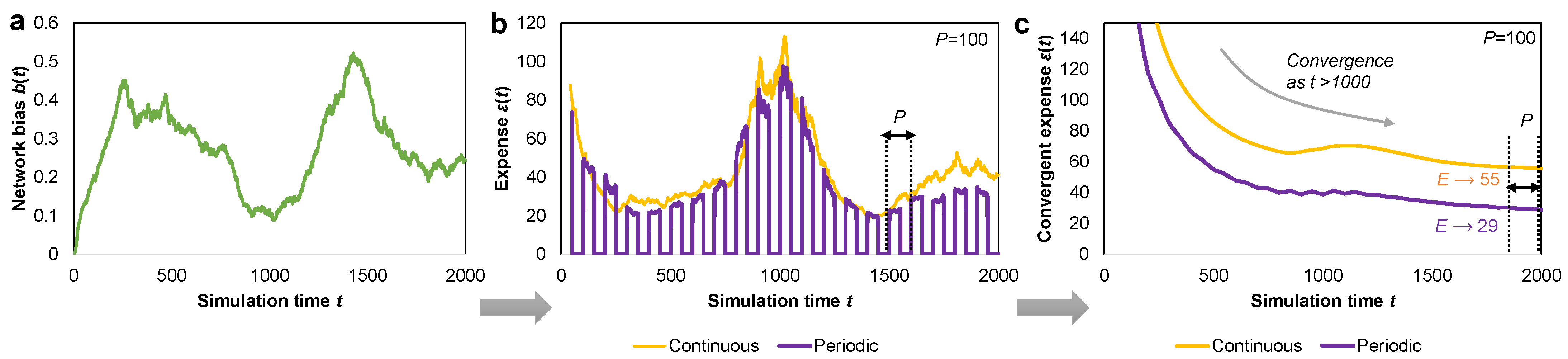
The conceptual difference between the two proposed injection strategies and the indoctrination expense that we measure is shown in Figure 1. In the illustrated example, given an arbitrary oscillating network bias , we measure the indoctrination expense in time for the two injection strategies. The main difference illustrated in Figure 1b is that the expense of the periodic strategy (violet) is similar in value to the expense of the continuous strategy (yellow) while the spreaders are active but drops to zero otherwise. Based also on the periodicity of spreader activation (here we use ), the convergent expense shown in Figure 1c drops in time and converges to the final indoctrination expense E. As an example, we suggest a final for the continuous injection and for the periodic injection. This further leads to an expense ratio of , suggesting that the continuous strategy is 89% less cost-effective than the periodic strategy in this example. In the Results section, we will discuss in terms of the measured E and the expense ratio between the two injection strategies.
2.3. Validation Datasets
We include 12 datasets in this study and divide them into three main categories: fundamental network topologies, complex synthetic network models, and real-world networks.
The chosen networks include the four fundamental topologies: the mesh , the Watts–Strogatz small-world [33], the random Erdös–Rényi network [34], and the Barabási–Albert scale-free network [35]. Next, we include four complex synthetic topologies: Holme–Kim [36], cellular [37], Watts–Strogatz with degree distribution [38], and Genosian [39] networks. Lastly, we choose four real-world networks: an online social network [40], a combined Facebook egonetwork [41], a scientific collaboration network in geometry [42] and an email communication network [43].
The motivation behind choosing the synthetic network models is the need for topological diversity. Therefore, the first four are reference models for network science, which we can understand and differentiate fundamentally based on differences in average path length, clustering coefficient, degree distribution and hub formation [44,45]. The latter four topologies combine the properties of the first and are able to reproduce more realistic networks in terms of communities, clustering, long-range links, etc. A representative network was generated for each of the eight synthetic networks; the algorithms and parameters for generating all these networks were selected according to each article cited where the models were first proposed and were implemented as Java plug-ins in Gephi [46] by the authors of this article.
The real-world datasets were chosen on the basis of diversity in size and context. Taking into account the high interest in the spread of influence, we chose four undirected networks consisting of various types of social relationships with sizes ranging from to 12,625 nodes and from to edges. In addition, we consider all regular spreader nodes as identical social agents, and only the network’s structural information is used in the simulation (such as node degree, adjacent edges), without any additional node-specific information (e.g., age, gender, professional status). A heterogeneous overview of the nodes in the network is beyond the goal of this paper but could represent a potential basis for further research.
Since we intend to understand the impact of the underlying topology from the cost-time perspective, we will often refer to the four fundamental topologies. Practically, all other networks (synthetic or real-world) can be considered a weighted combination of mesh, random, small-world, and scale-free networks [47]. In Table 1 we provide measurements for the characteristic network properties of each dataset. Here, we include the size of the network N, the number of edges E, the average degree , the maximum degree , the average path length , the average clustering coefficient , the modularity of the network (with default resolution [48]) and the diameter of the network [45].
3. Results
The benchmark results consist of repeated simulations that alternate between the following parameters: network topology, number of spreaders, spreader activity period and injection strategy. The 12 topologies used here are described in Table 1; the number of spreaders ranges in ; the spreader activity period ranges in ; we use the two injection strategies described in Section 2.2. Furthermore, the duration of the simulation is fixed at iterations, and the fill factor remains constant at . We made several considerations to simplify the analysis of all simulation results, such as: (i) considering one iteration as one ‘day’, (ii) a limitation in the maximum number of network datasets, (iii) a reasonable limitation for the number of spreaders (i.e., where corresponds to about 2% of all nodes in the network), (iv) a realistic activity period of no less than 5 days and no more than 250 days, (v) a standard fill factor of (i.e., spreaders may be active 50% of the time) (vi) and a long enough simulation duration to allow full convergence of the indoctrination expense. The motivation behind choosing each parameter is provided as follows:
- We observed that the convergent expense converges after iterations for all simulation settings. As such, a fixed value of is sufficient to capture the stable state of the network.
- The fill factor was given an intuitive fixed value of (50%) rather than any other intermediary value to reduce the complexity of the presented analysis. In addition, the goal of analyzing the effect of an alternative or dynamic fill factor may be the topic of a subsequent study.
- The number of spreaders was limited to , as a large enough value relative to the networks size (≈2%), beyond which it becomes implausible (in terms of cost) to maintain active agents in a network.
- The activity period P was fixed, considering that a minimum repetition period of less than 5 days (one work week) is hardly relevant for a commercial campaign, while a maximum effective period of 1–3 months was suggested in marketing studies [49]. Nevertheless, we chose several intermediary values up to 250 days (over 8 months).
To ensure statistical reliability, all experimental results represent average values measured over 100 repeated simulations using the same settings. Overall, we conducted a total of 12 (topologies) × 5 (spreader settings) × 6 (period settings) × 2 (injection strategies) × 100 (repetitions) = 72,000 experiments that correspond to 720 unique simulation settings. Hence, we opt for a graphical representation of the results in various settings instead of providing very long tables. To fully understand the impact of each simulation parameter, we study the results using the graphical representations in Figure 2, Figure 3, Figure 4, Figure 5 and Figure 6.
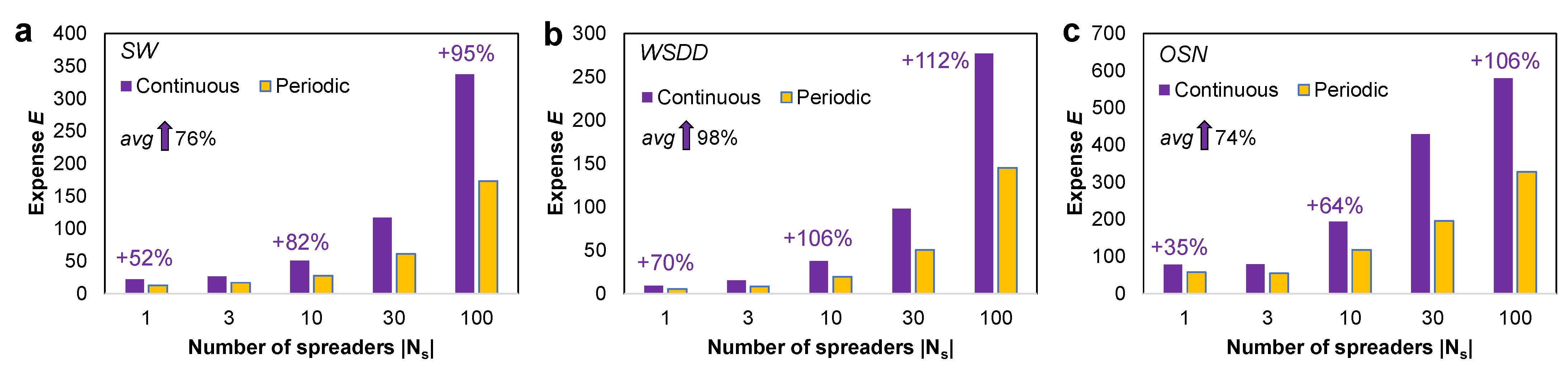
We first measure the indoctrination expense incurred by the two proposed opinion injection strategies, continuous and periodic. Figure 2 shows the increase in E as the number of spreaders increases. To exemplify the role of topologies, we selected a network from each of the three network categories, namely , , and . The numerical results on all 12 topologies support the conclusion that the continuous injection strategy (i.e., keeping spreaders active continuously) is less cost-effective than the periodic injection strategy. On average, the continuous strategy yields a 1.69–1.98 times higher expense E (that is, +69–98%) than the periodic strategy.
In addition, we note that both injection strategies incur a polynomial increase in expense E, while the number of spreaders increases linearly from 1 to 100. An intuitive real-world explanation is that doubling the number of spreaders does not double the spreading bandwidth or potential. There are several factors such as the positioning of the spreaders which have been shown to impact spreading efficiency [50] as well as topological characteristics such as hub formation, average path length, local clustering, etc. [6]. Consequently, our experiments confirm that higher spreader counts yield increasingly higher indoctrination expenses.
We measure average expense ratios between the continuous and periodic strategies of for fundamental topologies, for complex topologies, and for real-world topologies when using one single spreader. When using 100 spreaders, these expense ratios increase to 1.93, 1.92 and 2.11, respectively. Therefore, the expense difference between the two injection strategies increases by 15–42% when the number of spreaders is increased.
To better understand the difference between the two injection strategies as shown in Figure 2, we propose an intuitive numerical example. Say that during a continuous injection strategy with spreaders the network bias is , such that the indoctrination expense is according to Equation (3). During an equivalent periodic injection strategy, where spreaders are active only half of the time (i.e., similar to having 25 spreaders continuously), we would expect half of the network bias over the 0.5 opinion threshold, that is, . In other words, we confirm that , the same as above. However, if the simulation results suggest, for example, an average 82% decrease in expense, this translates to an actual for the periodic injection strategy in our example. In turn, this results in a higher network bias than expected: instead of the theoretically expected , which is much closer to the bias measured during the continuous strategy of . This type of cost-effectiveness is present on all datasets and can be explained through the inherent memory of the LT opinion interaction model, which continues to diffuse diminishing amounts of opinion even when the spreader nodes are inactive. A similar kind of residual diffusion has been found to be specific to human interaction and social networks [6,13].
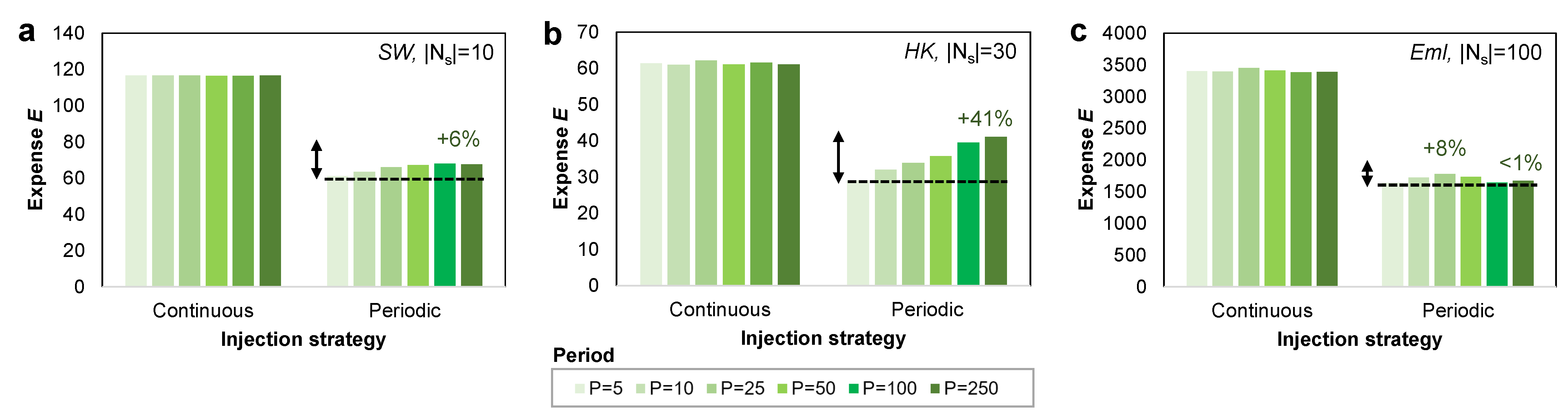
Next, in Figure 3, we analyze the impact of the spreader activity period P on the expense E. Compared to the continuous strategy, where the activity period has no significance, the periodic strategy suggests a small increase in expense E as P increases. The measured increases are usually within 0–20% from to ; two exceptions are the and networks with a more visible increase in expense of up to 39–41%. The average expense increase, when increasing P from 5 to 250 days, is 19.04% on the fundamental networks, 17.04% on the complex synthetic networks and 10.16% on the real-world networks. Consequently, the activity period has a smaller impact on the overall expense of indoctrination than the number of spreaders.
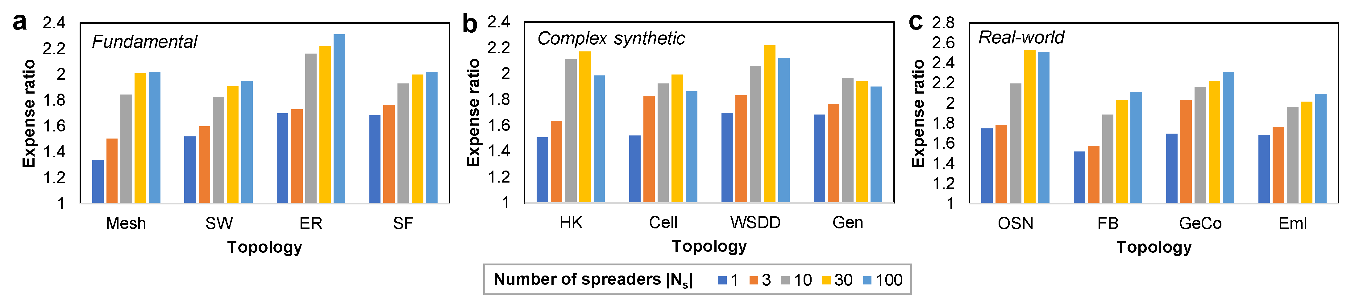
Another important observation is the impact of each topology. Figure 4 reveals two important aspects. First, we represent the expense ratio between the continuous and periodic injection strategies and notice a correlation between the increase in the expense ratio and the number of spreaders . In other words, the more spreaders introduced in a network, the less effective the continuous strategy becomes in comparison to the periodic one. In our experiments on the fundamental topologies, the periodic injection strategy is roughly 36% more cost-effective than the continuous one for spreader and increases to 51% (3 spreaders), 75% (10 spreaders), 93% (30 spreaders) and 93% (100 spreaders). On the complex topologies, the cost-effectiveness is 64%, 67%, 85%, 92% and 93% higher for the same number of spreaders; on the real-world networks, the cost-effectiveness is 53%, 72%, 76%, 105% and 111% higher.
When comparing the increases in the expense ratio between using one single spreader in the network up to 100 spreaders, we obtain an expense ratio increase of 33% for and 65% for , respectively, on the fundamental networks. The same expense ratio increases on the complex topologies are 23% for and 73% for ; on the real-world networks, these are 35% for and 105% for . In conclusion, the indoctrination expense ratio increases with the number of spreaders by an averaged 24% on the fundamental networks, 41% on the complex networks and 52% on the real-world networks.
The second observation extracted from Figure 4 is that we notice different patterns of increases in the expense ratio. Specifically, on the fundamental topologies, we observe that for the and networks in Figure 4a, the expense ratio follows a linear increase with the number of spreaders. On the network, the same increase is polynomial, and on the network, the expense ratio is higher and slightly logarithmic (convergent). Similar differences are visible on the other network categories, with higher overall expenses on the , and networks.
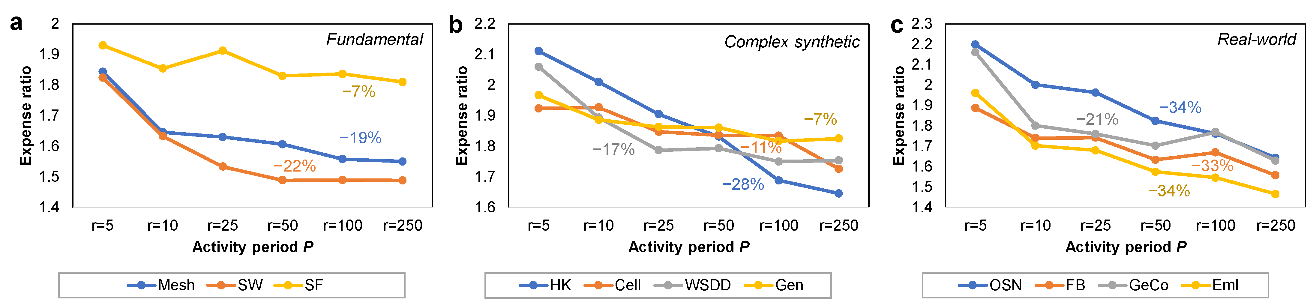
In Figure 5, we show the relationship between the expense ratio (between continuous and periodic injection strategies) and the activity period P for each of the three network categories. Overall, there is a clear decreasing trend in the expense ratio, meaning that the longer the activity period, the better the cost-effectiveness of the continuous strategy becomes compared to the periodic one.
On the fundamental topologies, the network has a non-deterministic response through simulation but yields higher expense ratios (of ≈2.5) than the other topologies. The network is also more expensive, and the expense ratio drops slightly. On the other hand, the and networks behave similarly, with a pronounced decrease of 19–22% decrease in the expense ratio as P increases. On the complex and real-world topologies, we measure significant drops in the expense ratios of 7–28% and 21–34%, respectively.
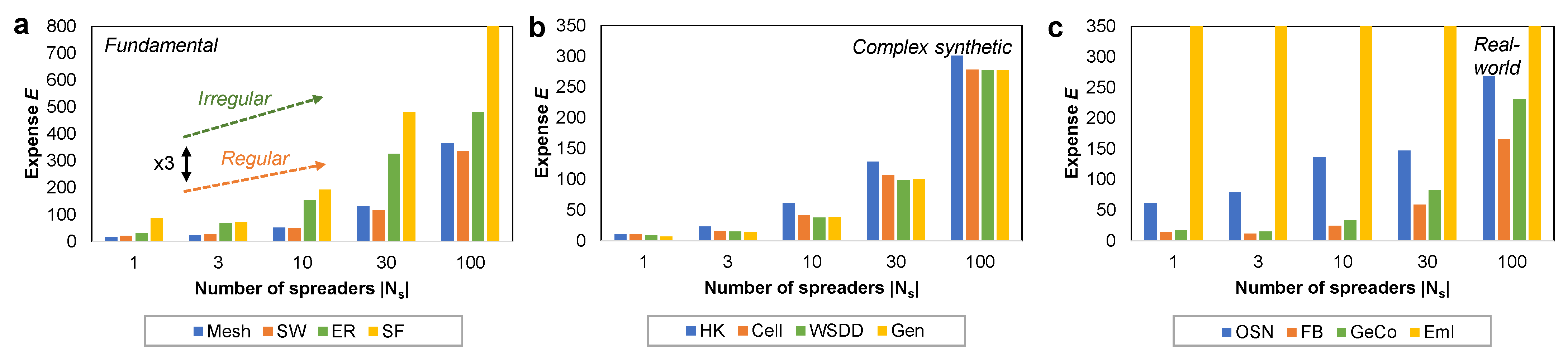
Finally, Figure 6 highlights the impact of the topology on the indoctrination expense E in association with an increasing number of spreaders. Figure 6a enables us to observe a distinctive signature of the and networks compared to the and networks. Taking into account the fundamental topological characteristics of each network [45], both and can be considered primarily as regular networks due to their high local clustering and non-power-law degree distributions. Similarly, the and networks display higher expenses E than the previous group. Both networks can be considered primarily irregular networks due to their low clustering and long-range links, even though is uniquely characterized by preferential attachment and a power-law degree distribution of node degrees [35].
An important remark is that the indoctrination expense E is approximately higher in the irregular group than in the regular group; more precisely, this ratio decreases from ( spreader) to ( spreaders). Regardless of , P, and injection strategy, the network always generates the highest indoctrination expense, followed by the network. A possible explanation is that in networks with preferential (or random) attachment, the selection of seeds is more important than in regular networks; namely, opinion diffusion becomes far more ineffective if spreaders do not coincide with hubs. Indeed, in real-world scenarios, choosing highly connected agents (e.g., influencers) as spreaders further implies much higher expenses; however, this analysis is currently beyond the scope of this paper. On networks, the lack of local clustering makes opinion diffusion challenging to control, indifferent to the location of spreaders.
In Figure 6b, we observe a relatively uniform scaling of E with the number of spreaders for every topology. All four networks induce expenses similar to the regular group in Figure 6a of 300. We note that all four complex synthetic networks are a combination of small-world and scale-free properties; nevertheless, the small-worldness of each seems to contribute to much smaller expenses than on the purely scale-free network.
The expenses measured on the real-world networks depicted in Figure 6c are quite insightful. All networks expect yield expenses E smaller than any of the other fundamental or complex synthetic networks for a large number of spreaders. Specifically, for , expenses range within , while expenses in the other two categories of networks range within (expect for ). The network is a “predominantly” scale-free collaboration network, therefore reminiscent of and a much higher expense E.
4. Discussion
Network science is a powerful interdisciplinary tool for modeling and better understanding real-world processes and is capable of revealing patterns in data that are hidden in classical statistical or analytical approaches [3,51]. Specifically, by employing network science, we are able to tackle the process of opinion diffusion, with overarching impact over topics such as controlling the spread of rumors, the spread of innovation, or even epidemic spreading, which are all highly impactful social and scientific challenges.
In this study, we augment the classic linear threshold model (LT) [20,21] with an original cost-time-aware framework to analyze the emerging trade-off between efficient opinion diffusion and cost of operation to minimize the indoctrination expense by maintaining active spreader nodes over a complex network. For this, we defined the bias of an agent node toward an opinion injected into the network (see Equation (1)) and the general bias of the network in time (see Equation (2)) as our discrete event simulation progresses. We introduced two mutually exclusive temporal opinion injection strategies—continuous and periodic—differentiated by the intermittent activity of spreaders in the network. The aim was to observe whether periodic activation of spreaders, given by a period parameter P, can reduce the overall indoctrination expense in time compared to a continuous activity, while ensuring that the network becomes biased toward the injected opinion. The differences between the two injection strategies are exemplified in Figure 1, and the converging and final E indoctrination costs are defined in Equations (4) and (5).
We implemented the simulation methodology based on the cost-time-aware LT model on three network categories: fundamental, complex synthetic and real-world. By alternating the topology, the number of spreaders, the spreader activity period and the injection strategy, we totaled 720 simulation scenarios. From the multitude of these experiments, we were able to extract relevant conclusions that could be used for cost-effective opinion injection in complex networks.
Our results show that the use of a periodic opinion injection strategy is preferential to a continuous one, as the first reaches a higher cost-effectiveness of +69–84% on average. Furthermore, periodic injection becomes even more effective as the number of spreaders relative to the continuous strategy increases from 58% with one spreader active to 99% with 100 spreaders active in the network. However, increasing the number of spreaders is proven to be less cost-effective—a higher opinion coverage may be achieved, but at polynomially increasing expense. By increasing the number of spreaders from 1 to 100, the expense increases approximately × 10–15 times (see Figure 2).
The underlying topology has a significant impact on the indoctrination expense. More precisely, in the fundamental topologies, two distinct signatures surface: regular networks (i.e., the and ) and irregular networks (i.e., the and networks). From the perspective of our study, the difference is that irregular networks generate indoctrination expenses E up to higher than regular networks. As a general rule, scale-free topologies generate the highest indoctrination expense, higher than random networks that generate higher expenses than and . The results in the fundamental topologies can be used to further interpret the results shown in Figure 6b,c. Basically, the other network categories (including the real-world networks) can be viewed as weighted combinations of the mesh, random, small-world and scale-free networks [47].
In terms of the activity period, we observe decaying expense ratios (between the continuous and periodic strategies) as the activity period P increases. This decrease is shown in Figure 5, where we measure drops in the expense ratio of 18% on fundamental, 14% on complex synthetic and 23% on real-world networks as P increases from 5 to 250. Networks with regularity in their underlying topology may trigger a higher decrease in expense ratio as the activity period increases, while irregular topologies will imply higher expense ratios and are less influenced by the activity period.
The general, patterns validated over all datasets are summarized as the following rules of thumb:
- The indoctrination expense increases (i.e., opinion diffusion becomes more expensive relative to its coverage):
- With the number of spreaders active in the network (polynomial increase) in our experiments, the expense increase was ×10–15 times from spreader to spreaders.
- By using a continuous injection strategy instead of a periodic one in our experiments, a periodic strategy with a 50% fill ratio is between 69–84% more cost-effective.
- Even though the impact is less significant, as the spreader activity period P increases to days (out of which spreaders are inactive half of the time), the expense drops by 0–20%.
- The expense ratio increases (i.e., the continuous strategy becomes less cost-effective relative to the periodic one):
- With the number of spreaders active in the network in our experiments, the expense ratio increases by 24–52% on average as increases from 1 to 100. In addition, irregular topologies (, ) cost more.
- With the decrease in spreader activity period P in our experiments, we measure drops in E of −14 to −23%, on average, as P increases from 5 to 250.
To better emphasize the practical advantage of a periodic injection strategy, we can imagine an example with two competing sides during an information campaign (e.g., marketing, political), say A and B. Party A has a very high budget, so they can afford to keep (and pay) a number of influencers continuously active in the social network. The second party has only half the budget, so they could afford to keep either influencers active continuously or adopt the same number of influencers by activating them periodically only half the time (i.e., incurring half the costs). In this second scenario, as supported by our experiments, the periodic strategy would be approximately 80% more cost-effective, which means that by halving the costs, the amount of indoctrination induced in the social network would be as much as 90% of the indoctrination induced by the first party with a double budget. More precisely, with only half the budget but an efficient timing strategy, party B achieves 90% of the same effect in the network as party A.
A similar example can be considered in terms of topological irregularity. As such, online social networks with powerful scale-free characteristics [52] will reduce the amount of indoctrination in the network to compared to a proximity-based social network with significant small-world characteristics [53]. In other words, each rule of thumb enumerated above should be carefully considered for the specific context for which it is applied.
In addition to the scientific potential of our benchmarking methodology, our results find real-world applicability in the context of influence maximization in key areas such as online marketing, where spreaders are injected into the network (e.g., human agents, influencers) or political campaigns where agents, or bots, act as sources of indoctrination [54]. Furthermore, the enumerated observations can be further generalized in computational epidemics, such as corroborating our injection strategies with isolation strategies and competing activation mechanisms in epidemics [55,56] or immunization strategies for viral outbreaks [57,58].
5. Conclusions
The design of cost-effective strategies for influence maximization in real-world networks is an ongoing scientific challenge [5,12,50,59] with an overarching impact on understanding information diffusion, controlling fake news and disease outbreaks and understanding the function of social networks as a whole [60,61,62,63,64]. In addition, real-world applications are often affected by the limitations of time, space and budget. Thus, finding trade-offs between a minimal number of influential nodes and a maximization of opinion coverage is a relevant scientific problem.
In this paper, we study the relationship between several specific parameters that influence the effectiveness of opinion diffusion, such as the nature of the underlying topology, the number of active spreaders, the periodicity of spreader activity, the duration of spreader activity and the injection strategy. Consequently, we implement an original benchmarking methodology by integrating time and cost awareness into an augmented linear threshold model and measuring the indoctrination expense as a trade-off between the cost to maintain active spreaders and real-time opinion coverage. The results of our discrete event simulations highlight distinct patterns that stimulate the increase in indoctrination expense. Specifically, we find that indoctrination expense increases with the number of spreaders, with the activity periodicity and by keeping spreaders active continuously rather than activating them periodically.
Taking into account the impressive amount of existing literature on influence maximization and opinion diffusion, we believe that our study represents a novel direction of research aimed at better understanding the real-world applicability of influence maximization strategies by incorporating realistic cost–time awareness. In general, we consider that our proposed methodology can trigger the creation of computational intelligence tools to further enhance strategies of opinion diffusion in complex networks.
Future research directions may include studying variable spreader costs in correlation with network centralities, implementing a mechanism to allow each spreader to activate independentl, and tuning of the amount of active spreaders in real-time according to various events in the network.
Funding
This research was funded by a grant of the Romanian Ministry of Research, Innovation and Digitalization, project number PFE 26/30.12.2021, PERFORM-CDI@UPT100—The increasing of the performance of the Polytechnic University of Timișoara by strengthening the research, development and technological transfer capacity in the field of “Energy, Environment and Climate Change” at the beginning of the second century of its existence, within Program 1—Development of the national system of Research and Development, Subprogram 1.2—Institutional Performance—Institutional Development Projects—Excellence Funding Projects in RDI, PNCDI III. Author A.T. was also partially supported by the Romanian National Authority for Scientific Research and Innovation (UEFISCDI), project number PN-III-P1-1.1-PD-2019-0379.
Institutional Review Board Statement
Not applicable.
Informed Consent Statement
Not applicable.
Data Availability Statement
All data used in this study is summarized in Table 1. The eight synthetic networks (fundamental and complex synthetic) were generated by the authors using custom plug-ins implemented in Gephi (to be shared on request to the corresponding author). The real-world networks are publicly available as follows: can be downloaded from the Github datasets repository https://github.com/gephi/gephi/wiki/Datasets (accessed 1 April 2022); , and can be downloaded from http://snap.stanford.edu/data/ (accessed 1 April 2022).
Conflicts of Interest
The author declares no conflict of interest.
References
- Granovetter, M.S. The strength of weak ties. Am. J. Sociol. 1973, 78, 1360–1380. [Google Scholar] [CrossRef] [Green Version]
- Barabási, A.L. Linked: The New Science of Networks; Basic Books: New York, NY, USA, 2002. [Google Scholar]
- Barabási, A.L. Network science. Philos. Trans. R. Soc. A Math. Phys. Eng. Sci. 2013, 371, 20120375. [Google Scholar] [CrossRef] [PubMed]
- Lazer, D.; Pentland, A.S.; Adamic, L.; Aral, S.; Barabasi, A.L.; Brewer, D.; Christakis, N.; Contractor, N.; Fowler, J.; Gutmann, M.; et al. Life in the network: The coming age of computational social science. Science 2009, 323, 721. [Google Scholar] [CrossRef] [PubMed] [Green Version]
- Chen, W.; Wang, Y.; Yang, S. Efficient influence maximization in social networks. In Proceedings of the 15th ACM SIGKDD International Conference on Knowledge Discovery and Data Mining, Paris, France, 28 June–1 July 2009; ACM: New York, NY, USA, 2009; pp. 199–208. [Google Scholar]
- Zhang, Z.K.; Liu, C.; Zhan, X.X.; Lu, X.; Zhang, C.X.; Zhang, Y.C. Dynamics of information diffusion and its applications on complex networks. Phys. Rep. 2016, 651, 1–34. [Google Scholar] [CrossRef] [Green Version]
- Sekara, V.; Stopczynski, A.; Lehmann, S. Fundamental structures of dynamic social networks. Proc. Natl. Acad. Sci. USA 2016, 113, 9977–9982. [Google Scholar] [CrossRef] [Green Version]
- González-Bailón, S.; Borge-Holthoefer, J.; Moreno, Y. Broadcasters and hidden influentials in online protest diffusion. Am. Behav. Sci. 2013, 57, 943–965. [Google Scholar] [CrossRef]
- Topîrceanu, A. Analyzing the Impact of Geo-Spatial Organization of Real-World Communities on Epidemic Spreading Dynamics. In Proceedings of the International Conference on Complex Networks and Their Applications, Madrid, Spain, 30 November–2 December 2020; Springer: Berlin/Heidelberg, Germany, 2020; pp. 345–356. [Google Scholar]
- Topirceanu, A. Electoral Forecasting Using a Novel Temporal Attenuation Model: Predicting the US Presidential Elections. Expert Syst. Appl. 2021, 182, 115289. [Google Scholar] [CrossRef]
- Kempe, D.; Kleinberg, J.; Tardos, É. Maximizing the spread of influence through a social network. In Proceedings of the Ninth ACM SIGKDD International Conference on Knowledge Discovery and Data Mining, Washington, DC, USA, 24–27 August 2003; ACM: New York, NY, USA, 2003; pp. 137–146. [Google Scholar]
- Morone, F.; Makse, H.A. Influence maximization in complex networks through optimal percolation. Nature 2015, 524, 65–68. [Google Scholar] [CrossRef] [Green Version]
- Hinz, O.; Skiera, B.; Barrot, C.; Becker, J.U. Seeding strategies for viral marketing: An empirical comparison. J. Mark. 2011, 75, 55–71. [Google Scholar] [CrossRef] [Green Version]
- Stonedahl, F.; Rand, W.; Wilensky, U. Evolving viral marketing strategies. In Proceedings of the 12th Annual Conference on Genetic and Evolutionary Computation, Portland, OR, USA, 7–10 July 2010; ACM: New York, NY, USA, 2010; pp. 1195–1202. [Google Scholar]
- Hartline, J.; Mirrokni, V.; Sundararajan, M. Optimal marketing strategies over social networks. In Proceedings of the 17th International Conference on World Wide Web, Beijing, China, 21–25 April 2008; ACM: New York, NY, USA, 2008; pp. 189–198. [Google Scholar]
- Bertsimas, D.; Lo, A.W. Optimal control of execution costs. J. Financ. Mark. 1998, 1, 1–50. [Google Scholar] [CrossRef]
- Aral, S.; Muchnik, L.; Sundararajan, A. Distinguishing influence-based contagion from homophily-driven diffusion in dynamic networks. Proc. Natl. Acad. Sci. USA 2009, 106, 21544–21549. [Google Scholar] [CrossRef] [PubMed] [Green Version]
- Guille, A.; Hacid, H. A predictive model for the temporal dynamics of information diffusion in online social networks. In Proceedings of the 21st International Conference on World Wide Web, Lyon, France, 16–20 April 2012; ACM: New York, NY, USA, 2012; pp. 1145–1152. [Google Scholar]
- Rodriguez, M.G.; Balduzzi, D.; Schölkopf, B. Uncovering the temporal dynamics of diffusion networks. arXiv 2011, arXiv:1105.0697. [Google Scholar]
- Granovetter, M. Threshold models of collective behavior. Am. J. Sociol. 1978, 83, 1420–1443. [Google Scholar] [CrossRef] [Green Version]
- Chen, W.; Yuan, Y.; Zhang, L. Scalable influence maximization in social networks under the linear threshold model. In Proceedings of the 2010 IEEE International Conference on Data Mining, Sydney, Australia, 13–17 December 2010; IEEE: New York, NY, USA, 2010; pp. 88–97. [Google Scholar]
- Guille, A.; Hacid, H.; Favre, C.; Zighed, D.A. Information diffusion in online social networks: A survey. ACM Sigmod Rec. 2013, 42, 17–28. [Google Scholar] [CrossRef]
- Goldenberg, J.; Libai, B.; Muller, E. Talk of the network: A complex systems look at the underlying process of word-of-mouth. Mark. Lett. 2001, 12, 211–223. [Google Scholar] [CrossRef]
- Holley, R.A.; Liggett, T.M. Ergodic theorems for weakly interacting infinite systems and the voter model. In The Annals of Probability; JSTOR: New York, NY, USA, 1975; pp. 643–663. [Google Scholar]
- Axelrod, R. The dissemination of culture: A model with local convergence and global polarization. J. Confl. Resolut. 1997, 41, 203–226. [Google Scholar] [CrossRef] [Green Version]
- Sznajd-Weron, K.; Sznajd, J. Opinion evolution in closed community. Int. J. Mod. Phys. C 2000, 11, 1157–1165. [Google Scholar] [CrossRef] [Green Version]
- Jackson, M.O.; Watts, A. The evolution of social and economic networks. J. Econ. Theory 2002, 106, 265–295. [Google Scholar] [CrossRef] [Green Version]
- Skyrms, B.; Pemantle, R. A dynamic model of social network formation. In Adaptive Networks; Springer: Berlin/Heidelberg, Germany, 2009; pp. 231–251. [Google Scholar]
- Topirceanu, A.; Udrescu, M.; Vladutiu, M.; Marculescu, R. Tolerance-based interaction: A new model targeting opinion formation and diffusion in social networks. PeerJ Comput. Sci. 2016, 2, e42. [Google Scholar] [CrossRef] [Green Version]
- Udrescu, M.; Topirceanu, A. Probabilistic Modeling of Tolerance-Based Social Network Interaction. In Proceedings of the Network Intelligence Conference (ENIC), 2016 Third European, Wrocław, Poland, 5–7 September 2016; IEEE: New York, NY, USA, 2016; pp. 48–54. [Google Scholar]
- Tako, A.A.; Robinson, S. Comparing discrete-event simulation and system dynamics: Users’ perceptions. In System Dynamics; Springer: Berlin/Heidelberg, Germany, 2018; pp. 261–299. [Google Scholar]
- Acemoğlu, D.; Como, G.; Fagnani, F.; Ozdaglar, A. Opinion fluctuations and disagreement in social networks. Math. Oper. Res. 2013, 38, 1–27. [Google Scholar] [CrossRef] [Green Version]
- Watts, D.J.; Strogatz, S.H. Collective dynamics of small-world networks. Nature 1998, 393, 440–442. [Google Scholar] [CrossRef] [PubMed]
- Erd6s, P.; Rényi, A. On the evolution of random graphs. Publ. Math. Inst. Hungar. Acad. Sci. USA 1960, 5, 17–61. [Google Scholar]
- Barabási, A.L.; Albert, R. Emergence of scaling in random networks. Science 1999, 286, 509–512. [Google Scholar] [CrossRef] [PubMed] [Green Version]
- Holme, P.; Kim, B.J. Growing scale-free networks with tunable clustering. Phys. Rev. E 2002, 65, 026107. [Google Scholar] [CrossRef] [PubMed] [Green Version]
- Tsvetovat, M.; Carley, K.M. Generation of Realistic Social Network Datasets for Testing of Analysis and Simulation Tools; Technical Report, DTIC Document; Defense Technical Information Center: Fort Belvoir, VA, USA, 2005.
- Chen, Y.; Zhang, L.; Huang, J. The Watts–Strogatz network model developed by including degree distribution: Theory and computer simulation. J. Phys. A Math. Theor. 2007, 40, 8237. [Google Scholar] [CrossRef]
- Topirceanu, A.; Udrescu, M.; Vladutiu, M. Genetically Optimized Realistic Social Network Topology Inspired by Facebook. In Online Social Media Analysis and Visualization; Springer: Berlin/Heidelberg, Germany, 2014; pp. 163–179. [Google Scholar]
- Opsahl, T.; Panzarasa, P. Clustering in weighted networks. Soc. Netw. 2009, 31, 155–163. [Google Scholar] [CrossRef]
- Leskovec, J.; Mcauley, J. Learning to discover social circles in ego networks. Adv. Neural Inf. Process. Syst. 2012, 25. [Google Scholar]
- Batagelj, V.; Mrvar, A. Pajek-program for large network analysis. Connections 1998, 21, 47–57. [Google Scholar]
- Leskovec, J.; Lang, K.J.; Dasgupta, A.; Mahoney, M.W. Community structure in large networks: Natural cluster sizes and the absence of large well-defined clusters. Internet Math. 2009, 6, 29–123. [Google Scholar] [CrossRef] [Green Version]
- Albert, R.; Jeong, H.; Barabási, A.L. Error and attack tolerance of complex networks. Nature 2000, 406, 378. [Google Scholar] [CrossRef] [Green Version]
- Wang, X.F.; Chen, G. Complex networks: Small-world, scale-free and beyond. IEEE Circuits Syst. Mag. 2003, 3, 6–20. [Google Scholar] [CrossRef] [Green Version]
- Bastian, M.; Heymann, S.; Jacomy, M. Gephi: An open source software for exploring and manipulating networks. In Proceedings of the Third International AAAI Conference on Weblogs and Social Media, San Jose, CA, USA, 17–20 May 2009. [Google Scholar]
- Topirceanu, A.; Duma, A.; Udrescu, M. Uncovering the fingerprint of online social networks using a network motif based approach. Comput. Commun. 2016, 73, 167–175. [Google Scholar] [CrossRef]
- Blondel, V.D.; Guillaume, J.L.; Lambiotte, R.; Lefebvre, E. Fast unfolding of communities in large networks. J. Stat. Mech. Theory Exp. 2008, 2008, P10008. [Google Scholar] [CrossRef] [Green Version]
- Chéron, E.; Kohlbacher, F.; Kusuma, K. The effects of brand-cause fit and campaign duration on consumer perception of cause-related marketing in Japan. J. Consum. Mark. 2012, 29, 357–368. [Google Scholar] [CrossRef]
- Topîrceanu, A. Competition-Based Benchmarking of Influence Ranking Methods in Social Networks. Complexity 2018, 2018, 4562609. [Google Scholar] [CrossRef]
- Topirceanu, A.; Udrescu, M. Statistical fidelity: A tool to quantify the similarity between multi-variable entities with application in complex networks. Int. J. Comput. Math. 2017, 94, 1787–1805. [Google Scholar] [CrossRef]
- Barabási, A.L. Scale-free networks: A decade and beyond. Science 2009, 325, 412–413. [Google Scholar] [CrossRef] [Green Version]
- Milgram, S. The small world problem. Psychol. Today 1967, 2, 60–67. [Google Scholar]
- Topîrceanu, A.; Precup, R.E. A novel geo-hierarchical population mobility model for spatial spreading of resurgent epidemics. Sci. Rep. 2021, 11, 14341. [Google Scholar] [CrossRef]
- Topirceanu, A.; Udrescu, M.; Marculescu, R. Centralized and decentralized isolation strategies and their impact on the COVID-19 pandemic dynamics. arXiv 2020, arXiv:2004.04222. [Google Scholar]
- Castellano, C.; Pastor-Satorras, R. Competing activation mechanisms in epidemics on networks. Sci. Rep. 2012, 2, 371. [Google Scholar] [CrossRef] [PubMed] [Green Version]
- Pastor-Satorras, R.; Vespignani, A. Immunization of complex networks. Phys. Rev. E 2002, 65, 036104. [Google Scholar] [CrossRef] [PubMed] [Green Version]
- Topîrceanu, A. Immunization using a heterogeneous geo-spatial population model: A qualitative perspective on COVID-19 vaccination strategies. Procedia Comput. Sci. 2021, 192, 2095–2104. [Google Scholar] [CrossRef] [PubMed]
- Topirceanu, A.; Udrescu, M.; Marculescu, R. Weighted Betweenness Preferential Attachment: A New Mechanism Explaining Social Network Formation and Evolution. Sci. Rep. 2018, 8, 10871. [Google Scholar] [CrossRef] [PubMed]
- Clarkson, J.J.; Tormala, Z.L.; Rucker, D.D.; Dugan, R.G. The malleable influence of social consensus on attitude certainty. J. Exp. Soc. Psychol. 2013, 49, 1019–1022. [Google Scholar] [CrossRef]
- Easley, D.; Kleinberg, J. Networks, Crowds, and Markets; Cambridge University Press: Cambridge, UK, 2010; Volume 8. [Google Scholar]
- Golbeck, J. Analyzing the Social Web; Elsevier: Amsterdam, The Netherlands, 2013. [Google Scholar]
- Kenett, D.Y.; Preis, T.; Gur-Gershgoren, G.; Ben-Jacob, E. Dependency network and node influence: Application to the study of financial markets. Int. J. Bifurc. Chaos 2012, 22, 1250181. [Google Scholar] [CrossRef]
- Topîrceanu, A. Breaking up friendships in exams: A case study for minimizing student cheating in higher education using social network analysis. Comput. Educ. 2017, 115, 171–187. [Google Scholar] [CrossRef]
Figure 1.
Conceptual representation of the methodology applied to calculate the indoctrination expense: (a) experimental measurement of the network bias toward one opinion (green); oscillations emerge due to the existence of multiple competing opinions (not shown here); (b) measured indoctrination expense for the continuous and periodic injection strategies; (c) from , we compute the convergent expense which begins to stabilize after approximately iterations; the final indoctrination expense E is calculated as an average of over the last P iterations.

Figure 2.
Comparison between the continuous (violet) and periodic (yellow) injection strategies, in terms of the indoctrination expense E, on three representative networks, one from each category (see Table 1): (a) small-world ; (b) Watts–Strogatz with degree distribution ; (c) online social network . The violet text represents the increase in expense E of the continuous strategy, namely the difference between the violet column and the adjacent yellow column. Measurements of E focus on the increase in the number of spreaders .

Figure 3.
Comparison between the two injection strategies, in terms of measured indoctrination expense E, highlighting the increase in the activity period P. Examples are chosen from each network category with a different number of spreaders : (a) small-world ; (b) Holme–Kim ; (c) Email network .
Figure 3.
Comparison between the two injection strategies, in terms of measured indoctrination expense E, highlighting the increase in the activity period P. Examples are chosen from each network category with a different number of spreaders : (a) small-world ; (b) Holme–Kim ; (c) Email network .

Figure 4.
The impact of each network topology on the expense ratio between the continuous and periodic injection strategies is shown in association with an increasing number of spreaders: (a) fundamental networks—the and show similar increases in the expense ratio, while the and networks suggest higher expense ratios; (b) complex synthetic networks—the shows a higher expense ratio, along with for a higher number of spreaders; (c) real-world networks—the and networks yield the lowest expense ratios.

Figure 5.
The impact of the spreader activity period P on the expense ratio between the continuous and periodic injection strategies is shown in association with each network topology: (a) fundamental networks, except the network whose expense ratios are significantly higher (≈2.5), not shown for graphical reasons; the and networks show similar drops in expense ratio; (b) complex synthetic networks—the network offers the highest drop in expense ratio as P increases; (c) real-world networks—all networks present similar drops in expense ratio.

Figure 6.
The indoctrination expense E is shown scaling with each topology grouped by the number of spreaders: (a) two distinct subcategories of networks are suggested over the fundamental networks—regular ( and with lower expenses) and irregular ( and with up to higher expenses); (b) complex synthetic networks—similar scaling of E with for all four networks; (c) real-world networks—higher E for the network, and much higher E for the network (in the order of .


Table 1.
Network measures for the validation datasets divided into fundamental, complex synthetic and real-world networks.
Table 1.
Network measures for the validation datasets divided into fundamental, complex synthetic and real-world networks.
| Dataset | Nodes | Edges | Average Degree | Maximum Degree | Average Path Length | Average Clustering Coefficient | Network Modularity | Network Diameter |
|---|---|---|---|---|---|---|---|---|
| 5000 | 25,234 | 5.047 | 36 | 13.942 | 0.185 | 0.855 | 37 | |
| 5000 | 19,998 | 4.000 | 11 | 10.607 | 0.426 | 0.829 | 22 | |
| 5000 | 20,923 | 4.185 | 21 | 4.253 | 0.002 | 0.418 | 8 | |
| 5038 | 19,198 | 3.811 | 174 | 4.275 | 0.020 | 0.536 | 10 | |
| 1000 | 3330 | 3.33 | 85 | 3.553 | 0.506 | 0.488 | 7 | |
| 1041 | 6012 | 5.775 | 95 | 4.428 | 0.258 | 0.885 | 10 | |
| 1178 | 9048 | 7.681 | 58 | 15.419 | 0.659 | 0.930 | 32 | |
| 1063 | 6915 | 6.505 | 25 | 4.765 | 0.498 | 0.882 | 9 | |
| 1899 | 20,296 | 10.688 | 339 | 3.055 | 0.138 | 0.338 | 8 | |
| 4039 | 88,234 | 43.691 | 1045 | 3.693 | 0.617 | 0.834 | 8 | |
| 3621 | 9461 | 5.226 | 102 | 5.316 | 0.679 | 0.743 | 14 | |
| 12,625 | 20,362 | 3.226 | 576 | 3.811 | 0.577 | 0.684 | 9 |
Publisher’s Note: MDPI stays neutral with regard to jurisdictional claims in published maps and institutional affiliations. |
© 2022 by the author. Licensee MDPI, Basel, Switzerland. This article is an open access article distributed under the terms and conditions of the Creative Commons Attribution (CC BY) license (https://creativecommons.org/licenses/by/4.0/).
Share and Cite
MDPI and ACS Style
Topîrceanu, A. Benchmarking Cost-Effective Opinion Injection Strategies in Complex Networks. Mathematics 2022, 10, 2067. https://doi.org/10.3390/math10122067
AMA Style
Topîrceanu A. Benchmarking Cost-Effective Opinion Injection Strategies in Complex Networks. Mathematics. 2022; 10(12):2067. https://doi.org/10.3390/math10122067
Chicago/Turabian StyleTopîrceanu, Alexandru. 2022. "Benchmarking Cost-Effective Opinion Injection Strategies in Complex Networks" Mathematics 10, no. 12: 2067. https://doi.org/10.3390/math10122067
Note that from the first issue of 2016, this journal uses article numbers instead of page numbers. See further details here.