A Survey on Characterizing Trees Using Domination Number

Abstract

Ever since the discovery of domination numbers by Claude Berge in the year 1958, graph domination has become an important domain in graph theory that has strengthened itself as a theory and has extended its contributions to various applications. Tree characterization is an important problem in graph domination. This survey focuses on presenting a collection of results on characterizing trees using domination number.

1. Introduction

In 1958, Claude Berge introduced the domination number in his book “Theory of Graphs and its Applications” [1]. Cockayne and Hedetniemi used the notation $\gamma$(G) to denote the domination number of graph G, which has become the most accepted notation. The literature on domination has been surveyed in detail in two eminent books by Haynes et al. [2,3]. There are various survey articles available in the literature of dominating sets. We find only few results on characterizing trees using a domination number. In this article, we have attempted to collectively provide a survey on the constructive characterization of trees using various types of domination numbers. We believe that this survey will be interesting for researchers interested in such characterizations. We could not include all the available tree characterizations. We apologize to the authors for the omission.

A graph G = (V, E) consists of a set of V = {v${}_1$, v${}_2$, ⋯} called vertices and another set E = {e${}_1$, e${}_2$, ⋯}, whose elements are called edges, such that each edge e${}_k$ is identified with an unordered pair (v${}_i$ v${}_j$) of vertices. The number of vertices is called the order of graph and denoted by |V| = n. The number of edges is called the size of the graph and denoted by |E| = m. For any set S of vertices of G, the induced subgraph 〈 S 〉 is the maximal subgraph of G with vertex set S. The degree of a vertex v denoted by d(v) is the number of vertices adjacent to v. The minimum and maximum degrees of vertices in V(G) are denoted by $\delta$(G) and Δ(G), respectively. A vertex v is said to be a weak support vertex if v is adjacent to exactly one pendant vertex; otherwise, v is called a strong support vertex. We denote the set of all pendant and support vertices of G by L(G) and S(G), respectively. The number of pendant and support vertices of G is denoted by $\mathit{l}$ and s, respectively. The distance d(u, v) between two vertices u and v in G is the length of the shortest path joining them. A vertex cover of a graph is a set D ⊆ V such that each edge of G is incident to at least one vertex of D. The vertex cover number of G, $\tau$(G), is the cardinality of a minimum vertex cover of G. The open neighborhood N(v) of the vertex v consists of the set of vertices adjacent to v, that is, N(v) = {u ∈ V(G) | (u v) ∈ E(G)}, and the closed neighborhood of v is N[v] = N(v) ∪ {v}. For any set S ⊆ V (G), its boundary B(S) = N(S) S. A graph is acyclic if it has no cycles. A tree is a connected acyclic graph. K${}_{1,n}$ denotes the star with n + 1 vertices. A tree is a double star if it contains exactly two vertices that are not pendant vertices if one of these vertices is adjacent to r pendant vertices and the other to s pendant vertices; then, we denote the double star by S${}_{r,s}$. P${}_n$, C${}_n$ and K${}_n$ denote the path, cycle and complete graph with n vertices, respectively.

The subdivision of some edge e with endpoints {u, v} yields a graph containing one new vertex w, with an edge set replacing e by two new edges: (u w) and (w v). A subdivision of a graph G is a graph resulting from the subdivision of edges in G. The vertex identification of a pair of vertices v${}_1$ and v${}_2$ in a graph produces a graph in which the vertices v${}_1$ and v${}_2$ are replaced with a single vertex v, such that v is adjacent to the union of the vertices to which v${}_1$ and v${}_2$ were originally adjacent. An edge contraction is an operation which removes an edge from a graph while simultaneously identifying the two vertices that it previously joined. For details on graph theory, we refer to [4,5].

A dominating set (DS) D of G is a set of vertices of G such that every vertex in V − D is adjacent to a vertex in D. If D has the smallest possible cardinality of any dominating set of G, then D is called a minimum dominating set—abbreviated as MDS. The cardinality of any MDS for G is called the domination number of G, and it is denoted by $\gamma$(G). A $\gamma$-set denotes a dominating set for G with minimum cardinality. The private neighborhood of v ∈ D, denoted by pn(v, D), is defined by pn(v, D) = N[v] − N[D − {v}]. A vertex v is said to be a down (critical) vertex if $\gamma$(G − v) < $\gamma$(G), a level vertex if $\gamma$(G − v) = $\gamma$(G) and an up vertex if $\gamma$(G − v) > $\gamma$(G). For details on domination, we refer to [2].

2. Survey

There are various types of dominating sets that have defined to date. Once a new type of dominating set is defined, researchers in general try to relate them to the existing dominating sets, leading to new types of dominating sets such as total restrained domination, independent domination critical, two-outer independent domination, double Roman domination, locating Roman domination, etc. Generally, tree characterizations are determined for:

• These types of dominating sets;
• Equal domination numbers for two different kinds of dominating sets.

While surveying the articles on tree characterization using dominating sets, we, in general, observe that the authors provide an iterative procedure for generating a tree T from a sequence of subtrees T${}_1$, T${}_2$, ⋯, T${}_i$, (i > 1). To generate these trees, T${}_1$, T${}_2$, ⋯, T${}_i$ are defined in general graph operations starting from an initial tree. The authors provide necessary and sufficient conditions for the existence of such trees and prove that the iterative tree characterization developed by them satisfies the particular dominating set property.

From this brief discussion, we understand that there have been hundreds of dominating sets defined to date, for which tree characterizations are attempted and determined in different ways. Based on the availability of these dominating sets, in this survey, we have attempted to provide a possible list characterizing 19 different types of dominating sets. We could not cover all the types of dominating sets in this short survey. We apologise to the authors for the omissions.

3. Tree Characterizations

To characterize trees using dominating sets, the general technique adopted is an iterative procedure of developing larger trees from smaller trees. For this, we start from some basic tree, such as P${}_1$, P${}_3$ and star graphs. At each stage of the iterative procedure, the resulting trees belong to the particular kind of domination. For example, if we begin with P${}_1$, and P${}_1$ has an independent dominating set, then this sequence of trees T${}_1$, T${}_2$, ⋯, T${}_j$ generated from P${}_1$ have independent dominating sets. For developing T${}_1$, T${}_2$, ⋯, T${}_j$, the general graph operations adopted are vertex merging, edge addition, adding a path between two trees and adding a sequence of vertices. For developing T${}_1$, T${}_2$, ⋯, T${}_j$, different authors define different kinds of graph operations (such as attaching a path P${}_i$, i = 1 to 5, attaching some tree structures, adding stars, etc.). This totally depends upon the type of dominating set used for developing these trees. We understand that even with the particular kind of dominating set, the graph operations adopted for developing these trees vary as other parameters are included. For example, the graph operations for a Roman domination number and double-Roman domination number will be different. In this section, we list out the graph operations and tree characterizations by various authors. We have grouped these graph operations into 19 different types based on a common dominating set share by various other possibilities as discussed in Section 2. Throughout this article:

• T${}_1$, T${}_2$, ⋯, T${}_j$, (j ≥ 1) is a sequence of trees.
• T${}_{i+1}$ can be generated recursively from T${}_i$ for i = 1, 2, ⋯, j − 1 using any one of the predefined operations.
• $\mathcal{T}$ is the family of trees obtained from a sequence T${}_1$, T${}_2$, ⋯, T${}_j$ (j ≥ 1).

Generally, while constructing $\mathcal{T}$, T${}_{i+1}$ can be obtained recursively from T${}_i$ and T${}_p$ either by merging or adding an edge between (u v), where u ∈ T${}_i$ and v ∈ T${}_p$. Figure 1 provides an example of the different types of domination to be discussed in this section.

For the graph G${}_1$ in Figure 1, every pair of two vertices is a $\gamma$-set: $\{1,3\}$ is an independent dominating set; $\{1,3\}$ is a 2-dominating set; $\{1,2,3,4\}$ is a double dominating set; $\left\{3\right\}$ is the Roman domination number; $\{1,2\}$ is a restrained dominating set; $\{1,2\}$ is a very excellent $\gamma$-set; and $\{1,2\}$ is a paired dominating set. The non-isolating two-bondage number of G is 1. Moreover, $\{1,2\}$ is a complementary tree dominating set, and $\{1,3\}$ is a disjunctive dominating set. G${}_1$ is a domination subdivision stable graph. G${}_1$ is also a $\gamma$-uniquely colorable graph. Finally, $\{1,2\}$ is a total dominating set, and {(1 2), (3 4)} is an edge-dominating set.

For the graph G${}_2$ in Figure 1, $\left\{2\right\}$ is a unique minimum dominating set. G${}_2$ is a domination dot stable graph. G${}_2$ is also a non-domination subdivision stable graph.

3.1. Independent Domination

Berge and Ore formalized the theory of independent domination in 1962 [1,6]. A dominating set D is said to be an independent dominating set (i(G)-set) if no two vertices in D are adjacent. The independent domination number is the minimum cardinality of an independent dominating set of G. Fricke et al. defined an i-excellent graph [7]. A graph G is i-excellent if every vertex of G belongs to some i(G)-set. In 2002, Haynes et al. provided a constructive characterization of i-excellent trees. For any vertex v of T, Haynes et al. defined the status of v as sta(v) = A for all support vertex of v or sta(v) = B for all pendant vertex v of T. Let $\mathcal{T}$${}_1$ be the family of trees such that T${}_1$ is a double star S${}_{r,r}$ for r ≥ 1, and T${}_{i+1}$ can be obtained from T${}_i$ by one of the Operations 1 or 2 [8].

Operation 1.

Attach a star K${}_{1,t}$ to T for t ≥ 1 by adding an edge between x and y, where x is the center of K${}_{1,t}$ and y ∈ V(T) and sta(y) = A, and t – 1 new pendant vertices adjacent to y. Let sta(x) = A and sta(v) = B for each new pendant v that was added to T.

Operation 2.

Attach S${}_{t,t+1}$ to T by adding an edge between x and y, where x ∈ V(S${}_{t,t+1}$) is adjacent to t ≥ 0 pendant vertices and y ∈ V (T) with sta (y) = B. Let sta(v) = A if v ∈ S(S${}_{t,t+1}$) ∪ {x}, and let sta(v) = B for each new pendant v that was added to T.

In Theorems 1 and 2, we present properties satisfied by T ∈ $\mathcal{T}$${}_1$ and a characterization of i-excellent trees.

Theorem 1

([8]). Let T ∈ $\mathcal{T}$${}_1$ and let u and v be vertices of T with sta(u) = A and sta(v) = B. Then:

1. 

T is an i-excellent tree.

2. 

There is an i(T)-set that contains N(u).

3. 

There is an i(T)-set S such that v ∈ S and pn(v, S) = $\left\{v\right\}$.

Theorem 2

([8]). A tree T is i-excellent if and only if T ∈ {K${}_1$, K${}_2$} or T ∈ $\mathcal{T}$${}_1$.

It is to be noted that although i-excellent trees are excellent, the family of $\gamma$-excellent trees is properly contained in the set of all i-excellent trees. The double star S${}_{r,r}$ for r ≥ 2 is an example of an i-excellent tree that is not $\gamma$-excellent.

In i-excellent trees, T${}_1$ is a star graph, and the sequence of trees is also obtained by attaching star graphs only. We observe that when edges are subdivided, this is not the case.

Sharada et al. introduced the concept of independent domination critical and stable graphs upon edge subdivision [9]. A graph is an independent domination edge subdivision critical (i-critical) if the subdivision of an arbitrary edge increases the independent domination number. In 2015, Sharada provided a constructive characterization of i-critical trees. Let $\mathcal{T}$${}_2$ be the family of trees such that T${}_1$ is a star K${}_{1,t}$ for t > 1 and T${}_{i+1}$ obtained from T${}_i$ by one of the Operations 3 or 4 [10].

Operation 3.

Attach a path (u v x) to T by adding an edge between x and y, where y ∈ V(T) such that sta(y) = B. Let sta(u) = B, sta(v) = A and sta(x) = B.

Operation 4.

Attach a path (u v w x) to T by adding an edge between x and y, where y ∈ V(T) such that sta(y) = A. Let sta(u) = B, sta(v) = A and sta(w) = sta(x) = B.

In Theorems 3 and 4 and Corollary 1, we provide properties of i-critical trees and a characterization of T ∈ $\mathcal{T}$${}_2$.

Theorem 3

([10]). A tree T is i-critical if and only if there is a unique minimum-independent dominating set in T.

Corollary 1

([10]). Let T be a tree of order at least three. Then, the following conditions are equivalent:

1. 

T belongs to the family $\mathcal{T}$${}_2$.

2. 

T is i-critical.

3. 

There is exactly one minimum independent dominating set in T.

Theorem 4

([10]). If T is a tree T with at least three vertices, then T ∈ $\mathcal{T}$${}_2$ if and only if there is a unique minimum-independent dominating set in T.

Theorem 4 provides a new insight that this theorem can be consider as a characterization of trees having a single dominating set that is also independent.

For a secure dominating set, the operations slightly vary by attaching a star or a path when T${}_1$ is a path. The problem of secure domination was introduced by Cockayne et al. [11]. A dominating set D of a graph G is said to be a secure dominating set (SDS) if each vertex u ∈ V − D is adjacent to a vertex v ∈ D such that (D − v) ∪ {u} is a DS of G. The secure domination number $\gamma$${}_s$(G), is the minimum cardinality of an SDS of G. An SDS of G of cardinality $\gamma$${}_s$(G) is called a $\gamma$${}_s$-set of G. If u ∈ V(T) is not a pendant of T and k = min{d${}_T$(u, v): v ∈ V(T) and v is a pendant of T}, then u is called a k-stem of T. A one-stem is called a stem of T. In 2017, Zepeng et al. provided a constructive characterization of trees with equal independent and secure domination numbers. Let $\mathcal{T}$${}_3$ be the family of trees such that T${}_1$ is P${}_4$ and T${}_{i+1}$ can be obtained from T${}_i$ by one of the Operations 5–7 [12].

Operation 5.

Attach a path (u x) to T by adding an edge between x and y, where y is a stem or a 2-stem of T.

Operation 6.

Attach R${}_k$ to T by adding an edge between x and y, where x is a stem or 2-stem of T and y is a 2-stem of R${}_k$, where k ≥ 2, (where R${}_k$ is a k-star with each edge subdivided twice).

Operation 7.

Attach R${}_k$ to T by merging a pendant edge of T and a pendant edge of R${}_k$ to a single edge, where k ≥ 2.

In Theorems 5 and 6, we present results relating independent trees and secure domination trees.

Theorem 5

([12]). If T ∈ $\mathcal{T}$${}_3$, then γ(T) = i(T) = γ${}_s$(T).

Theorem 6

([12]). Let T be a tree with at least three vertices. Then γ(T) = i(T) = γ${}_s$(T) if and only T ∈ $\mathcal{T}$${}_3$.

Sometimes, the construction becomes simple by generating the entire tree with the single operation, as in the case of independent dominating edge lift stable. Here, P${}_2$ is attached to generate the entire tree. The process of edge lifting, or sometimes called edge splitting, was introduced by Lovasz [13,14]. Let u and v be any two vertices in G at a distance 2 apart, and let x be a common neighbor of both u and v. Then, uxv is an induced path in G. An edge lifting defined on uxv is the process of removing the edges ux and xv while adding the edge uv to E(G). The edges ux and vx are said to be lifted off the vertex x. A graph is an independent domination edge lift stable if the lifting of an edge leaves the independent domination number of the graph unchanged. In 2018, Sharada provided a constructive characterization of trees which are independent domination edge lift stable.

The authors label the vertices of T ∈ $\mathcal{T}$${}_4$ as follows. Initially if T = P${}_4$, then sta(v) = A if v is a support vertex of T and sta(v) = B if v is a leaf of T. Let $\mathcal{T}$${}_4$ be the family of trees, and T${}_{i+1}$ can be obtained from T${}_i$ by Operation 8 [15].

Operation 8.

Let T be a path (a b c d) in $\mathcal{T}$${}_4$. Extend it by attaching a path (v w x) and the edge (u v) where sta(u) = B and u ∈ T. Then sta(v) = sta(w) = A and sta(x) = B.

In Theorems 7 and 8, we present results relating independent domination edge lift stable trees.

Theorem 7

([15]). If T ∈ $\mathcal{T}$${}_4$ and T${}^{uv}$${}_x$ is the tree obtained by the independent domination edge lifting of uv of x, then i (T${}^{uv}$${}_x$) = i(T). That is, T is an independent domination edge lift stable tree.

Theorem 8

([15]). T is an independent domination edge lift stable tree if and only T ∈ $\mathcal{T}$${}_4$.

3.2. Two-Domination

While developing the iterative procedures, sometime researchers have a unique and different approach in developing the tree operations. Few of such graph operations is presented in this Section on two-dominating sets.

The concept of a k-dominating set was first introduced by Fink and Jacobson in 1985 [16]. A vertex in V-D is k-dominated if it is dominated by at least k-vertices in D, that is, |N(v) ∩ D |≥ k. If every vertex in V-D is k-dominated, then D is called a k-dominating set. The k-domination number $\gamma$${}_k$(G) is the minimum cardinality of a k-dominating set of G. A subset S of V(G) is k-independent if the maximum degree of the subgraph induced by the vertices of S is less or equal to k - 1. The maximum cardinality of a k-independent set of G is the k-independence number $\beta$${}_k$(G). In 2011, Chellali et al. provided a tree characterization that satisfies the condition $\gamma$${}_2$(T) = $\gamma$${}_1$(T) + 2. The authors developed an elegant characterization by attaching paths of different length between two trees T${}_1$ and T${}_2$. They developed nine different operations for this purpose. These operations are developed by defining four families of trees. A summarized view is presented here. They defined the following notations.

Let B(T) be the set of subdivided vertices. Let A(T) = V(T) − B(T). Let F be the family of extremal trees such that:

• $\gamma$${}_2$(T) = $\gamma$(T) + 1;
• F = F${}_1$ ∪ F${}_2$ ∪ F${}_3$, where F${}_1$, F${}_2$ and F${}_3$ are subdivided stars, the corona of stars and the subdivided double stars of F, respectively.

Let X = X(T) consist of the pendant vertices adjacent to the vertex of maximum degree if F in F${}_2$, where F = P${}_2$ and X = ∅ otherwise; let H = H(T) consist of the center vertex if F ∈ F${}_3$ and H = ∅ otherwise.

They defined the family of $\mathcal{G}$${}_1$ = ⋃${}^4$${}_{i=1}$ G${}_i$, where G${}_1$ is the family of trees obtained by a path P${}_2$ = (u v) and a tree T ∈ F different to the path P${}_4$, by adding an edge (u w), where w ∈ B(T) − H(T). G${}_2$ is the family of trees obtained by a tree T ∈ F different to the path P${}_2$ by adding a new vertex attached to any support vertex of T. G${}_3$ is the family of trees obtained by a path P${}_3$ and a tree T ∈ F${}_2$∪ F${}_3$ different to P${}_2$ and P${}_4$ by adding an edge (x y), where x is any pendant vertex of P${}_3$ and y ∈ L(T) − X. G${}_4$ is the family of trees that are a subdivision graph of a caterpillar having three or four support vertices, and the remaining vertices of the caterpillar are pendant vertices. The family of $\mathcal{T}$${}_5$ can be constructed using one of the Operations 9–17 [17].

Operation 9.

Let T${}_1$, T${}_2$ ∈ F, each of an order of at least three. Form T from T${}_1$ ∪ T${}_2$ by adding an edge between x and y, where x ∈ B(T${}_1$) − H(T${}_1$) and y ∈ B(T${}_2$) − H(T${}_2$).

Operation 10.

Let T${}_1$, T${}_2$ ∈ F${}_1$. Form T from T${}_1$ ∪ T${}_2$ by adding an edge between x and y, where x ∈ V(T${}_1$) and y ∈ A(T${}_2$).

Operation 11.

Let T${}_1$ ∈ F${}_3$ and T${}_2$ ∈ F${}_1$. Form T from T${}_1$ ∪ T${}_2$ by adding an edge between x and y, where x ∈ H(T${}_1$) and y ∈ A(T${}_2$).

Operation 12.

Let T${}_1$ ∈ F, T${}_2$ ∈ F${}_2$ ∪ F${}_3$, with T${}_2$ ≠ P${}_2$. Form T from T${}_1$ ∪ T${}_2$ by adding an edge between x and y, where x ∈ B(T${}_1$) − H(T${}_1$) and y ∈ A(T${}_2$) − L(T${}_2$).

Operation 13.

Let T${}_1$, T${}_2$ ∈ F, each of order at least four. Form T from T${}_1$ ∪ T${}_2$ by adding an edge between x and y, where x ∈ A(T${}_1$) − L(T${}_1$) and y ∈ A(T${}_2$) − L(T${}_2$), or x ∈ L(T${}_1$) − X and y ∈ A(T${}_2$) − L(T${}_2$) and at least T${}_1$ or T${}_2$ ∈ F${}_1$.

Operation 14.

Let T${}_1$ ∈ F${}_2$, T${}_2$ ∈ F but not both a path P${}_2$. Form T from T${}_1$ ∪ T${}_2$ by adding a path (x z y), where x is a vertex of a maximum degree in T${}_1$, y ∈ A(T${}_2$) − X(T${}_2$) and z is a new vertex.

Operation 15.

Let T${}_1$ ∈ F${}_1$, T${}_2$ ∈ F${}_3$. Form T from T${}_1$ ∪ T${}_2$ by adding a path (x v w z y), where v, w and z are new vertices; x ∈ A(T${}_1$); y ∈ A(T${}_2$); and at least one of x and y is not in L(T${}_1$) ∪ L(T${}_2$) or x ∈ L(T${}_1$), y ∈ L(T${}_2$); and T${}_1$ = P${}_3$.

Operation 16.

Let T${}_1$ ∈ F${}_1$ and T${}_2$ ∈ F${}_1$. Form T from T${}_1$ ∪ T${}_2$ by adding a path (x v w z y), where x ∈ A(T${}_1$) and y ∈ A(T${}_2$).

Operation 17.

Let T${}_1$ ∈ F${}_3$ and T${}_2$ ∈ F${}_3$. Form T from T${}_1$ ∪ T${}_2$ by adding a path (x v w z y), where x ∈ A(T${}_1$) − L(T${}_1$) and y ∈ A(T${}_2$) − L(T${}_2$).

In Theorems 9 and 10, we present results relating the two-domination number of trees.

Theorem 9

([17]). A tree T satisfies γ${}_2$(T) = γ(T) + 2 if and only if T ∈ $\mathcal{G}$${}_1$ ∪ $\mathcal{T}$${}_5$

Theorem 10

([17]). A tree T satisfies γ${}_{\delta }$ (T) = γ(T) + 2 if and only if T ∈ $\mathcal{G}$${}_1$ ∪ ($\mathcal{T}$${}_5$ − $\mathcal{T}$${}_5$${}^{{}^{\prime }}$), where $\mathcal{T}$${}_5$${}^{{}^{\prime }}$ is the sub family of $\mathcal{T}$${}_5$ consisting of all trees constructed by performing Operation 9.

In 2012, Chellali et al. characterized ($\gamma$${}_2$, $\beta$${}_2$)-trees. A tree with equal two-domination and two-independence numbers is said to be ($\gamma$${}_2$, $\beta$${}_2$) tree. Let $\mathcal{T}$${}_6$ be the family of trees such that T${}_1$ is a star K${}_{1,t}$, where (t ≥ 1) and T${}_{i+1}$ can be obtained from T${}_i$ by one of the Operations 18–21 [18].

Operation 18.

Attach a star K${}_{1,t}$, where (t ≥ 2) to T by adding an edge between x and y, where x is the center of the star and y is an arbitrary vertex of T.

Operation 19.

Attach a double star S${}_{1,\mathit{l}}$ with support vertices u and x to T by adding an edge between x and y, where y is an arbitrary vertex of T, with the condition that if γ${}_2$(T − y) = γ${}_2$(T) − 1. Then, no neighbor of y in T belongs to a γ${}_2$(T − y)-set.

Operation 20.

Attach a path (u x) to T by adding an edge between x and y, where y is a pendant vertex of T that belongs to every β${}_2$(T)-set with the condition that β${}_2$(T − v) + 1 = β${}_2$(T).

Operation 21.

Attach a path (u w x) to T by adding an edge between x and y, where y ∈ γ${}_2$(T)-set and satisfies further γ${}_2$(T − y) ≤ γ${}_2$(T) with the condition that if γ${}_2$(T − y) = γ${}_2$(T) − 1, then no neighbor of y in T belongs to a γ${}_2$(T − y)-set.

In Lemma 1 and Theorem 11, the author provided the ($\gamma$${}_2$, $\beta$${}_2$) tree characterization in terms of global properties.

Lemma 1

([18]). If T ∈ $\mathcal{T}$${}_6$, then γ${}_2$(T) = β${}_2$(T).

Theorem 11

([18]). Let T be a tree of order n. Then γ${}_2$(T) = β${}_2$ (T) if and only if T = K${}_1$ or T ∈ $\mathcal{T}$${}_6$.

Note that Theorem 11 provides a constructive characterization for the upper bound of the characterization $\gamma$${}_2$(T) ≤ $\beta$${}_2$(T) [16].

In 2017, Brause et al. provided a constructive characterization of the same with respect to local properties of the tree at each stage of the construction. The authors have gracefully used the operations of edge addition in six different operations. For this purpose, they defined 25 different trees to make the characterization possible. The results are summarized and presented here.

Let A = {T${}_1$, T${}_2$ ⋯, T${}_{15}$} and B = {B${}_1$, B${}_2$ ⋯, B${}_{10}$} be the graphs as seen in Figure 2. Let T${}_p$ ∈ A ∪ B be a special tree, and let T be a tree. If T contains a subset U of vertices such that T[U] ≡ T${}_p$ and the degree of every black vertex in V${}_B$(T${}_p$) equals its degree in T, then we say that the tree T contains T${}_p$ as a prescribed-degree-induced subtree, abbreviated as PDI-subtree. In particular, we note that if T${}_p$ is a PDI-subtree of a tree T, then the degree sequence of the vertices of V${}_B$(T${}_p$) in T equals the degree sequence of the vertices of V${}_B$(T${}_p$) in T${}_p$. Let $\mathcal{T}$${}_7$ be the family of trees such that T${}_{i+1}$ can be obtained from T${}_i$ by one of the Operations 22–27 [19].

Operation 22.

Let T${}_p$ ∈ {T${}_1$, T${}_2$, T${}_8$} be a PDI-subtree of T${}^{{}^{\prime }}$ and v = v(T${}_p$). Add a pendant edge at v and label the pendant vertex as u.

Operation 23.

Let T${}_p$ ∈ {T${}_4$, T${}_{11}$, T${}_{12}$, T${}_{13}$, T${}_{15}$} be a PDI-subtree of T${}^{{}^{\prime }}$ and v = v(T${}_p$). Attach a path (u v x) to T${}^{{}^{\prime }}$ by adding an edge between x and v.

Operation 24.

Attach a path (u x v) to T${}^{{}^{\prime }}$ by adding an edge between x and y, where y is an arbitrary vertex of T${}^{{}^{\prime }}$.

Operation 25.

Let T${}_p$ ∈ {T${}_1$, T${}_2$, T${}_3$, T${}_5$, T${}_6$, T${}_7$, T${}_9$ and T${}_{10}$} be a PDI-subtree of T${}^{{}^{\prime }}$ and v = v(T${}_p$). Attach a path (x u w) to T${}^{{}^{\prime }}$ by adding an edge between x and v.

Operation 26.

Let T${}_p$ ≡ T${}_6$ be a PDI-subtree of T${}^{{}^{\prime }}$ and let v${}_1$ = v${}_1$(T${}_p$) and v${}_2$ = v${}_2$(T${}_p$). Attach a path (x u) to T${}^{{}^{\prime }}$ by adding an edge between x and v${}_1$. Add a pendant edge at v${}_2$ and label the pendant vertex as u${}_2$.

Operation 27.

Let T${}_p$ ≡ T${}_{14}$ be a PDI-subtree of T${}^{{}^{\prime }}$ and let v${}_1$ = v${}_1$(T${}_p$), v${}_2$ = v${}_2$(T${}_p$). Remove the edge (v${}_1$ v${}_2$), and attach a path (u x w) by adding edges between and the vertices (u v${}_1$) and (x v${}_2$).

In Theorems 12 and 13, the author provided the ($\gamma$${}_2$, $\beta$${}_2$) tree characterization in terms of local properties.

Theorem 12

([19]). If T is obtained from an arbitrary tree T${}^{{}^{\prime }}$ by applying one of the operations in the family of $\mathcal{T}$${}_7$, then β${}_2$(T) − γ${}_2$(T) = β${}_2$(T${}^{{}^{\prime }}$) − γ${}_2$(T${}^{{}^{\prime }}$).

Theorem 13

([19]). A tree is a (γ${}_2$, β${}_2$)-tree if and only if T ∈ $\mathcal{T}$${}_7$.

This characterization depends only on local properties of a tree at every stage of construction. This varies from the characterization of [18], which uses global properties of a tree which involves properties of minimum two-dominating set and maximum two-independent set in the tree at each stage of the construction.

Another interesting characterization, where the authors have attempted to add a set of l + 1 new vertices in their operations is presented here. As explained in [20], the annihilation number of a graph was first introduced by Pepper [21]. The annihilation number $\alpha$(G) is the largest integer k such that the sum of the first k terms of the non-decreasing degree sequence of G is at most |E(G)|. The upper annihilation number of a graph G is defined as the largest integer k such that the sum of the first k terms of the degree sequence of G arranged in non-decreasing order is at most |E(G)| + 1, and it is denoted by $\alpha$${}^{*}$(G). In 2014, W. J. Desormeaux et al. characterized the trees relating the annihilation number and the two-domination number of T. Initially, they had constructed the family $\mathcal{T}$${}_{i,j}$ of trees such that T${}_{2,j}$ ∈ $\mathcal{T}$${}_{i,j}$, where T${}_{2,j}$ is a double star S${}_{1,j-1}$ and 2 ≤ i ≤ j. Let $\mathcal{T}$${}_8$ = {K${}_2$} ∪ (⋃${}_{i\ge 2}$ T${}_i$), where T${}_i$ = ⋃${}_{j\ge i}$ $\mathcal{T}$${}_{i,j}$ be the family of trees such that T${}_{i+1}$ can be obtained from T${}_i$ by one of the Operations 28 and 29 [22].

Operation 28.

If v ∈ V(T) is a pendant vertex in T, then adding the set {t, s${}_1$, s${}_2$, ⋯, s${}_l$} of $\mathit{l}$ + 1 new vertices to V(T), where l ≥ i − 1 is arbitrary and adding an edge between t and s${}_1$, and the edges between v and s${}_i$, for all i = 1, 2, ⋯, $\mathit{l}$ to E(T). Add the resulting tree to the family T${}_{i,min\{j,l+1\}}$.

Operation 29.

If v ∈ V(T) has d(v) ≤ min {i, j − 1}, then adding the set {t, s${}_1$, s${}_2$, ⋯, s${}_{\mathit{l}}$} of $\mathit{l}$ + 1 new vertices to V(T), where $\mathit{l}$ ≥ max {d(v) + 1, i} − 1 is arbitrary and adding an edge between t and v, and the edges between t and s${}_i$ for all i = 1, 2, ⋯, $\mathit{l}$ to E(T). Add the resulting tree to the family $\mathcal{T}$${}_{max\left\{d\right(v)+1,i\},min\{j,\mathit{l}+1\}}$.

Theorems 14 and 16 provide upper bounds for ${\gamma }_2$(T) and Theorem 15 provides a characterization of T ∈ $\mathcal{T}$${}_8$.

Theorem 14

([22]). For a tree T, the following hold:

1. 

γ${}_2$(T) ≤ α${}^{*}$(T);

2. 

γ${}_2$(T) ≤ α(T) + 1.

Theorem 15

([22]). ${\gamma }_2$(T) = α(T) + 1 if and only if T ∈$\mathcal{T}$${}_8$.

Theorem 16

([22]). If T is a tree, then γ${}_2$(T) ≤ $(n+\mathit{l})$/2 with equality if and only if T ∈ {K${}_2$} ⋃ (⋃${}_{j\ge 2}$$\mathcal{T}$${}_{2,j}$).

This characterization proves that the conjecture ${\gamma }_2$(T) ≤ $\alpha$(T) + 1 is true when G is a tree.

The study of two-outer-independent domination was initiated by Jafari Rad [23]. A subset D ⊆ V(G) is a two-outer-independent dominating set (2OIDS) of G denoted by $\gamma$${}_2$${}^{oi}$(G)-set, if every vertex of an independent set V-D has at least two neighbors in D. The two-outer-independent domination number $\gamma$${}_2$${}^{oi}$ is the minimum cardinality of a 2OIDS of G. In 2015, Krzywkowski provided a constructive characterization of trees with equal two-domination and two-outer-independent domination numbers. Let $\mathcal{T}$${}_9$ be the family of trees such that T${}_1$ is any tree that belongs to the family of trees in which, for every pair of adjacent vertices of a degree of at least three, at least one of them has an even number of pendant vertices. T${}_{i+1}$ can be obtained from T${}_i$ using the Operation 30 [24].

Operation 30.

Attach a star K${}_{1,t}$ to T by joining x with y, where x is the center of a star, each edge of a star can be subdivided by any non-negative even number of times and y belongs to some γ${}_2$${}^{oi}$(T)-set.

In Theorems 17 and 18, we provide results relating two-domination and two-outer-independent domination numbers.

Theorem 17

([24]). If T ∈ $\mathcal{T}$${}_9$, then γ${}_2$${}^{oi}$(T) = γ${}_2$(T).

Theorem 18

([24]). Let T be a tree. γ${}_2$${}^{oi}$(T) = γ${}_2$(T) if and only if T ∈ $\mathcal{T}$${}_9$.

3.3. Double Domination

In this section on double domination, the authors have used vertex properties to develop the graph operations. Harary et al. initiated the study on double domination in graphs [25]. A double-dominating set is a dominating set that dominates every vertex of G at least twice. The minimum cardinality of a double-dominating set of G is the double domination number $\gamma$${}_{\times 2}$(T). Haynes et al. introduced a paired domination number in 1998 [26]. A paired-dominating set of a graph G is a dominating set of vertices whose induced subgraph has a perfect matching. The minimum cardinality of a paired dominating set of G is the paired domination number $\gamma$${}_{pr}$(T). In 2006, Blidia et al. provided a constructive characterization for trees with equal paired and double domination numbers. The authors have used support and pendant vertices for defining Operations 31–33. Let C(T${}_1$) = ∅. Let $\mathcal{T}$${}_{10}$ be the family of trees such that T${}_1$ is P${}_2$ and T${}_{i+1}$ can be obtained from T${}_i$ by one of the Operations 31–33 [27].

Operation 31.

Attach a path (u v x) to T by adding an edge between x and y, where y is a support vertex of T. Let C(T${}_{i+1}$) = C(T${}_i$) ∪ {w}.

Operation 32.

Attach a path (u x) to T by adding an edge between x and y, where y is an arbitrary vertex of C(T${}_i$). C(T${}_{i+1}$) = C(T${}_i$)

Operation 33.

Attach a path (u v x w z) to T by adding an edge between x and y, where y is arbitrary vertex of C(T${}_i$). Let C(T${}_{i+1}$) = C(T${}_i$) ∪ {x}.

Note that for every i, 1 ≤ i ≤ k, C(T${}_i$) is the set of vertices of Ti that are neither support vertices nor leaves.

In Theorems 19 and 20, we provide results relating double domination and paired domination numbers and a characterization of T ∈ $\mathcal{T}$${}_{10}$. The paired and double domination numbers are generally not comparable. The authors have provided an illustration to support this. This characterization proves the conjecture that $\gamma$${}_{pr}$(T) = $\gamma$${}_{\times 2}$(T).

Theorem 19

([27]). For any tree T, the following statements are equivalent:

1. 

γ${}_{pr}$(T) = γ${}_{\times 2}$(T);

2. 

T = P${}_2$ or every support vertex of T is adjacent to exactly one pendant, no pair of support vertices of T are adjacent and T has a unique γ${}_{\times 2}$(T)-set consisting of the support and pendant vertices of T;

3. 

T ∈ $\mathcal{T}$${}_{10}$.

Theorem 20

([27]). For any tree T, γ${}_{pr}$(T) = γ${}_{\times 2}$(T) if and only if T ∈ $\mathcal{T}$${}_{10}$.

Around the same time, Chellali provided a constructive characterization for attaining the upper bounds of double domination trees in terms of pendant and support vertices. They also characterized the trees attaining the lower bound. The author claims that this theorem gives a sense of good framing on the double domination number in trees. The results are presented here. Let $\mathcal{T}$${}_{11}$ be the family of trees such that T${}_1$ is P${}_2$ and T${}_{i+1}$ can be obtained from T${}_i$ by one of the Operations 34 and 35 [28].

Operation 34.

Attach a vertex x to T by adding an edge between x and y, where y is any support vertex of T.

Operation 35.

Attach a path (u v x) to T by adding an edge between x and y, where y is an arbitrary vertex of T with the condition that if y is a pendant vertex of T, then its support vertex is not strong in T.

We note that the properties of support vertices are used to define these operations. We present the bounds on double domination number using the number of pendant and support vertices in Theorem 21. Theorem 22 provides a tree characterization of T ∈ $\mathcal{T}$${}_{11}$.

Theorem 21

([28]). If T ∈ $\mathcal{T}$${}_{11}$, then S(T) is a γ${}_{\times 2}$(T)-set of size (2n + l − s + 2)/3.

Theorem 22

([28]). If T is a non-trivial tree of order n, then γ${}_{\times 2}$(T) ≥ (2n + $\mathit{l}$ − s + 2)/3 with equality if and only if T ∈ $\mathcal{T}$${}_{11}$.

Based on the suggestions of Chellali, Krzywkowski provided a necessary condition so that the double domination number of a tree is equal to this its two-domination number plus one. He also provided a constructive characterization of these trees, which is presented here.

In 2012, Krzywkowski provided a constructive characterization of trees with a double domination number equal to the two-outer-independence number. Let T be a tree. If T is a path, then let C(T) be a one-element set containing a support vertex of T. If T is not a path, then let C(T) be a set of vertices of T which have degree at least three. Two vertices of C(T) are linked if the path joining them in T such that all interior vertices have a degree two. Then, the path is called a link. The length of a link is the number of its edges. We call paths joining pendant vertices of T to vertices of C(T) chains. The length of a chain is the number of its edges. Let $\mathcal{G}$${}_2$ be the family of trees such that every link has length two, every chain has a length of one or three and each vertex of C(T) is adjacent to at least one chain of length one. Let $\mathcal{T}$${}_{12}$ be the family of trees that either belong to the family $\mathcal{G}$${}_2$, or can be obtained from an element of $\mathcal{G}$${}_2$, say T${}^{{}^{\prime }}$, using one of the Operations 36 or 37. In both the operations, x denotes a pendant vertex of T${}^{{}^{\prime }}$ [29]. In these two operations, the property of N(y) of vertex y is also used for developing the operations.

Operation 36.

Attach a vertex x to T by adding an edge between x and y, where y is a pendant vertex of T such that the neighbor of y is a strong support vertex or has a degree at least three.

Operation 37.

Attach a tree F of the family $\mathcal{G}$${}_2$ to T by adding an edge between x and y, where y is a pendant vertex of T such that the neighbor of y is the strong support vertex and x is any pendant vertex in F.

In Theorem 23, we provide results relating double domination and two-domination numbers. Theorem 24 provides a constructive characterization of T ∈ $\mathcal{T}$${}_{12}$.

Theorem 23

([29]). If T ∈ $\mathcal{T}$${}_{12}$, then γ${}_{\times 2}$(T) = γ${}_2$(T) + 1.

Theorem 24

([29]). Let T be a tree. γ${}_{\times 2}$(T) = γ${}_2$(T) + 1 if and only if T ∈ $\mathcal{T}$${}_{12}$.

3.4. Roman Domination

Roman domination was formally defined by Cockayne et al. [30]. Let f: V → {0, 1, 2} be a function of G. The weight of f is w(f) = ∑${}_{v\in V}$ f(v), and let V${}_i$ = {v ∈ V: f(v) = i} for i = 0, 1, 2. The function f is a Roman dominating function if, for every vertex v ∈ V${}_0$, there exists u ∈ N(v) ∩ V${}_2$. The Roman domination number, denoted by ${\gamma }_R$(G), is the minimum weight among all Roman dominating functions on G. A slightly different approach of generating operations from rooted trees is used by Henning et al. They also used vertex properties to define the operations.

In 2002, M. A Henning provided a constructive characterization of Roman trees. Let $\mathcal{G}$${}_3$ denote the family of all rooted trees such that every pendant vertex different from the root is at distance 2 from the root and all children, except possibly one, of the root are a strong support vertex. Let $\mathcal{G}$${}_4$ denote the family of all rooted trees such that every pendant is at distance 2 from the root and all but two children of the root are strong support vertices. Let S ⊆ G and let V${}_S$(T) = {v ∈ V(T), v ∈ S(T) and ${\gamma }_R$(T – v) ≥ ${\gamma }_R$(T)}. Let $\mathcal{T}$${}_{13}$ be the family of trees such that T${}_1$ is K${}_{1,r}$ for r ≥ 1 and T${}_{i+1}$ can be obtained from T${}_i$ by one of the Operations 38–40 [31]. Pendant and central vertex properties are used for defining these operations.

Operation 38.

Attach a star K${}_{1,t}$, t ≥ 2 to T by adding an edge between x and y, where x is the center of K${}_{1,t}$ and y ∈ V${}_S$(T).

Operation 39.

Attach a tree F of the family $\mathcal{G}$${}_3$ to T by adding an edge between x and y, where x is an arbitrary vertex of T and y is the pendant vertex of F if F = P${}_3$ or y is the central vertex of T if F ≠ P${}_3$.

Operation 40.

Attach a tree F of the family $\mathcal{G}$${}_4$ to T by adding an edge between x and y, where x denotes the central vertex of T and y ∈ V${}_S$(T).

In Theorem 25, we provide a constructive characterization of T ∈ $\mathcal{T}$${}_{13}$.

Theorem 25

([31]). A tree T is a Roman tree if and only if T ∈ $\mathcal{T}$${}_{13}$.

Theorem 25 gives a solution to the open problem posted by Hedetniemi at the ninth quadrennial international conference in June 2000.

A double Roman dominating function (DRDF) is a function f: V → {0, 1, 2, 3}, if f(v) = 0 for a vertex v, then v has at least two adjacent vertices assigned 2 under f or one adjacent vertex assigned 3 under f. If f(v) = 1, then v has at least one neighbor with f(w) ≥ 2. The weight of a DRDF is defined as the sum f(V) = ∑${}_{u\in V}$ f(v) and the minimum weight of a DRDF on G is the double Roman domination number of G, denoted by ${\gamma }_{dR}$(G).

In 2019, M. A. Henning and N. Jafari Rad provided a constructive characterization of double Roman trees, which provided the answer for the question posted by Beller et al. [32] in 2016. Let $\mathcal{G}$${}_5$ be the tree shown in Figure 3. For k ≥ 2, let $\mathcal{G}$${}_6$ be the tree obtained from k vertex disjoint copies of a path P${}_5$ by adding a new vertex u and joining it to the central vertex of each path. When k = 2, the tree $\mathcal{G}$${}_6$ is illustrated in Figure 3. The vertex u in $\mathcal{G}$${}_5$ and $\mathcal{G}$${}_6$ (k ≥ 2) are labeled the pivot vertex of the tree.

Let $\mathcal{T}$${}_{14}$ be the family of trees and T${}_{i+1}$ can be obtained from T${}_i$ by one of the Operations 41–50 [33]. Different vertex properties such as strong the support vertex, central vertex and pendant vertex are used to define the operations.

Operation 41.

Attach a vertex x to T by adding an edge between x and y, where y is the strong support vertex of T.

Operation 42.

Attach a path (u x v) to T by adding an edge between x and y, where y is a vertex of T that is at distance of 2 from a pendant vertex in T where the common neighbor of y and the pendant vertex have degree 2 in T.

Operation 43.

Attach a path (u v x) to T by adding an edge between x and y, where y is an arbitrary vertex of T.

Operation 44.

Attach a path (u x v) to T by adding an edge between x and y, where y is a strong support vertex of T.

Operation 45.

Attach a path (u x v) to T by adding an edge between x and y, where y is an arbitrary vertex T that is adjacent to a strong support vertex of degree 3 in T with its two neighbors different from y both being pendant vertices in T.

Operation 46.

Attach a star K${}_{1,3}$ to T by adding an edge between x and y, where x is a pendant in K${}_{1,3}$ and y is an arbitrary vertex of T.

Operation 47.

Attach a double star S${}_{2,2}$ by adding an edge between x and y, where x is a pendant vertex of S${}_{2,2}$ and y is an arbitrary vertex of T that cannot be assigned the value 3 under any ${\gamma }_R$-function of T.

Operation 48.

Attach a tree $\mathcal{G}$${}_5$ to T by adding an edge between x and u, where u is the pivot vertex of $\mathcal{G}$${}_5$ and x is the vertex of T that belongs to no γ-set of T and that is assigned the value 0 in every ${\gamma }_R$-function of T.

Operation 49.

Attach a path (u x) to T by adding an edge between x and y, where y is a vertex of T such that the following holds. Firstly, the vertex y is the central vertex of a path P${}_5$ in T where the degree of every vertex on this path is the same as its degree in T except for exactly one pendant of the path which has degree at least 2 in T Secondly, every γ${}_{dR}$-function of T assigns to the vertex y the value 0.

Operation 50.

Attach a tree $\mathcal{G}$${}_6$, for some k ≥ 2 to T by adding an edge between x and y, where x is the pivot vertex of $\mathcal{G}$${}_6$ and y is an arbitrary vertex of T that belongs to some γ-set of T.

In Theorem 26, we provide a constructive characterization of T ∈ $\mathcal{T}$${}_{14}$.

Theorem 26

([33]). A tree T is a double Roman tree if and only if T ∈ $\mathcal{T}$${}_{14}$.

Adding a single edge helped in defining graph operations in many characterizations related to Roman domination. These results are presented here. A generalization of Roman domination under the name Italian domination was introduced in [34], where the authors called it Roman {2}-domination. The function f is said to be a Roman {2}-dominating function if, for every vertex v ∈ V${}_0$, ∑${}_{u\in N\left(v\right)}$ f(u) ≥ 2. The Roman {2}-domination number, denoted by ${\gamma }_{2R}$(G), is the minimum weight among all Roman {2}-dominating functions on G. The Italian domination number of G is denoted by ${\gamma }_I$(G). In 2017, M. Hajibaba et al. provided a constructive tree characterization of Italian and double-Roman domination numbers that satisfies the condition ${\gamma }_I\left(T\right)$ = 2${\gamma }_{dR}$(T)/3. Let $\mathcal{T}$${}_{15}$ be the family of trees such that T${}_1$ is a double star K${}_{1,t}$ for t ≥ 2 and T${}_{i+1}$ can be obtained from T${}_i$ by one of the Operations 51 and 52 [35]. We note that edge addition is used in these operations.

Operation 51.

Let ${\gamma }_I$(T − y) ≥ ${\gamma }_I$(T). Attach a star K${}_{1,t}$, t ≥ 2 to T by joining x with y, where x is the center vertex of K${}_{1,t}$, where t ≥ 2.

Operation 52.

Attach a star K${}_{1,t}$, t ≥ 1 to T by joining x with y, where x is the center vertex of K${}_{1,t}$ and y is an arbitrary vertex of T, and then subdividing the new edge.

In Theorems 27 and 28, we provide a bound for double Roman domination and a constructive characterization of T ∈ $\mathcal{T}$${}_{15}$.

Theorem 27

([35]). For every graph G, γ${}_{dR}$(G)/2 ≤ γ${}_I$(G) ≤ 2γ${}_{dR}$(G)/3.

Theorem 28

([35]). If T is a tree of order n ≥ 3, then γ${}_I$(T) = 2γ${}_{dR}\left(T\right)$/3 if and only if T ∈ $\mathcal{T}$${}_{15}$.

The authors have provided an infinite family of trees that achieve the equality for the lower bound. They have also proven that if $\gamma$${}_{dR}$(G)/2 = $\gamma$${}_I$(G), then $\gamma$${}_I$(G) = $\gamma$${}_2$(G), V${}_2$ = ∅ for every $\gamma$${}_I$(G)-function f = (V${}_0$, V${}_1$, V${}_2$) and have shown that the converse is not valid.

The locating Roman dominating function was introduced by Jafari Rad [36]. An RDF f = (V${}_0$, V${}_1$, V${}_2$) is called a locating Roman dominating function (or just LRDF) if N(u) ∩ V${}_2$ ≠ N(v) ∩ V${}_2$ for any pair u, v of distinct vertices of V${}_0$. The locating Roman domination number $\gamma$${}^L$${}_R$(G) is the minimum weight of an LRDF of G. In 2018, Jafari Rad et al. provided a constructive tree characterization of the locating Roman domination number that satisfies the condition $\gamma$${}^L$${}_R$(T) = (4n + l + s)/5. The authors define a vertex w of degree at least two in a tree T is called a special vertex if the following conditions hold:

• If f(w) = 2 for a $\gamma$${}^L$${}_R$(G)-function f = (V${}_0$, V${}_1$, V${}_2$), then pn(w, V${}_0$) ≠ ∅.
• If f(w) = 1 for a $\gamma$${}^L$${}_R$(G)-function f = (V${}_0$, V${}_1$, V${}_2$), then N(w) ∩ V${}_2$) = ∅.

Let $\mathcal{T}$${}_{16}$ be the family of trees such that T${}_1$ is P${}_4$, and T${}_{i+1}$ can be obtained from T${}_i$ by one of the Operations 53–56 [37]. We note that edge addition is used in these operations.

Operation 53.

Attach a vertex x to T by adding an edge between x and y, where y is a support vertex of T.

Operation 54.

Attach a path P${}_5$ to T by joining x with y, where x is a pendant vertex od P${}_5$ and y is a pendant vertex in T.

Operation 55.

Attach a path P${}_2$ to T by joining x with y, where x is a pendant vertex of P${}_2$ and y is a special vertex of T.

Operation 56.

Attach a path P${}_9$ to T by joining x with y, where x is the central vertex of P${}_9$ and y is an arbitrary vertex of T, d(T) ≥ 2 and γ${}^L$${}_R$(T − w) ≥ γ${}^L$${}_R$(T).

In Theorems 29 and 30, we present a bound for locating Roman domination with respect to number of vertices, pendant and support vertices and a constructive characterization of T ∈ $\mathcal{T}$${}_{16}$.

Theorem 29

([37]). For any tree T of order n ≥ 2, γ${}_R$${}^L$(T) ≤ (4n + l + s)/5.

Theorem 30

([37]). For a tree T of order n ≥ 2, γ${}_R$${}^L$(T) = (4n + $\mathit{l}$ + s)/5 if and only if T = K${}_{1,n-1}$ or T ∈ $\mathcal{T}$${}_{16}$.

In 2019, A. C. Martinez et al. provided a constructive characterization of trees with equal Roman domination {2} and a Roman domination number.

A near Roman {2}-dominating function relative to a vertex v, abbreviated near-R2DF relative to v, on a graph G = (V, E) is a function f = (V${}_0$, V${}_1$, V${}_2$) satisfying the following. For each vertex u in V such that f(u) = 0, if u = v, then ${\sum }_{u\in N\left(v\right)}$ f(u) ≥ 1, while if u ≠v, then ${\sum }_{u\in N\left(v\right)}$ f(u) ≥ 2. The weight of a near-R2DF relative to v on G is the value f(V) = ${\sum }_{u\in N\left(v\right)}$ f(u). The minimum weight of a near-R2DF relative to v on G is called the near Roman {2}-domination number relative to v of G, which the authors denotes $\gamma$${}^n$${}_R$(G;v). The authuors used stable and near vertex for their discussions, and it can be defined as follows. A vertex v is said to be a stable vertex in G, if $\gamma$${}_R$(G − v) ≥ $\gamma$${}_{R2}$(G), while v is a near stable vertex in G if $\gamma$${}^n$${}_R$(G;v) = $\gamma$${}_{R2}$(G). Let $\mathcal{T}$${}_{17}$ be the family of trees such that T${}_1$ is P${}_3$ and T${}_{i+1}$ can be obtained from T${}_i$ by one of the Operations 57–62 [38]. We note that edge addition is used in these operations.

Operation 57.

Attach a star K${}_{1,3}$ to T by adding an edge between x and y, where x is a pendant vertex of K${}_{1,3}$ and y is an arbitrary vertex of T.

Operation 58.

Attach a double star S${}_{1,2}$ to T by adding an edge between x and y, where x is the weak support vertex of S${}_{1,2}$ and y is an arbitrary vertex of T.

Operation 59.

Attach a path (u x v) to T by adding an edge between x and y, where y is a stable vertex of T.

Operation 60.

Attach a path (u v x) to T by adding an edge between x and y, where y is a near stable vertex of T.

Operation 61.

Attach a vertex x to T by adding an edge between x and y, where y ∈ S${}_{2,R}$(T).

Operation 62.

Attach a vertex x to T by adding an edge between x and y, where y ∈ L(T) is a near stable vertex.

In Theorem 31, the author provided a necessary and sufficient for the graph G satisfying the equality $\gamma$${}_{2R}$(G) = $\gamma$${}_R$(G). Also in Theorem 32, they provided a constructive tree characterization of T ∈ $\mathcal{T}$${}_{17}$.

Theorem 31.

Let G be a graph. Then, γ${}_{2R}$(G) = γ${}_R$(G) if and only if there exists a γ${}_{2R}$(G) function f = (V${}_0$, V${}_1$, V${}_2$) such that V${}_0$, V${}_1$ = ∅.

Theorem 32

([38]). A tree of order n ≥ 3, γ${}_{2R}$(T) = γ${}_R$(T) if and only if T ∈ $\mathcal{T}$${}_{17}$.

3.5. Restrained Domination

The concept of restrained domination was introduced by Telle et al. [39]. He had studied it as a vertex partitioning problem. In 1999, G. S. Domke et al. labeled the same problem as restrained domination. A set D ⊆ V is a restrained dominating set if every vertex not in D is adjacent to a vertex in D and to a vertex in V-D. The restrained domination number $\gamma$${}_r$(G) is the minimum cardinality of a restrained dominating set of G [40]. As observed in Section 3.4, in this section, all the graph operations also depend on a single edge addition. In 2000, G. S. Domke et al. provided a constructive characterization of trees for restrained domination number. Let $\mathcal{T}$${}_{18}$ be the family of trees such that $\gamma$${}_r$(T) = $⌈\frac{n+2}{3}⌉$. For k = 1, 2, let T${}_k$ be the tree obtained from K${}_{1,3}$ by subdividing k edges once. T${}_{i+1}$ can be obtained from T${}_i$ by one of the Operations 63 or 64.

Operation 63.

Attach a path P${}_2$ at y, where y is a vertex of T not belonging to some minimum restrained dominating set.

Operation 64.

Attach a path P${}_3$ at y, where y belongs to some minimum restrained dominating set of T.

Later, they defined three families of trees as follows. Let G${}_1$ be the family of trees with order 3k, which can be obtained from the tree T${}_2$ by a finite sequence of Operation 64. Let G${}_2$ be the family of trees with order 3k + 1, which can be obtained from P${}_4$ by a finite sequence of operations 64. Let G${}_3$ be the family of trees with order 3k + 2, which can be obtained from P${}_5$ or from the tree T${}_1$ by a finite sequence of operations 64 with the union of the family of trees with order 3k + 2, which can be constructed from the tree T${}_2$ by a finite sequence of Operation 64, followed by Operation 63 and then by a finite sequence of Operation 64. Let $\mathcal{G}$${}_7$ be the family of trees obtained from G${}_1$, G${}_2$ or G${}_3$ [41].

In Theorems 33 and 34, we present a bound for restrained domination and a constructive characterization of T ∈ $\mathcal{T}$${}_{18}$.

Theorem 33

([41]). If T is a tree of order n ≥ 1, then γ${}_r$(T) ≥ ⌈$\frac{n+2}{3}$⌉.

Theorem 34

([41]). A tree of order n ≥ 4, $\mathcal{T}$${}_{18}$ = $\mathcal{G}$${}_7$.

Pushpam and Padmapriea et al. introduced the concept of restrained Roman domination in graphs [42]. An RDF, f = (V${}_0$, V${}_1$, V${}_2$) on a graph G is a restrained Roman dominating function, or just rRDF on G if every vertex of V${}_0$ has a neighbor in V${}_0$. The restrained Roman domination number of G ${\gamma }_{rR}$(G), is the minimum weight of an rRDF on G. In 2011, Jafari Rad et al. provided a constructive characterization of a restrained Roman domination number of trees that satisfies the condition ${\gamma }_{rR}$(T) ≥ (2n + $\mathit{l}$ − s + 4)/3. Let $\mathcal{T}$${}_{19}$ be the family of trees such that T${}_1$ ∈ {P${}_4$, P${}_5$, P${}_6$} and T${}_{i+1}$ can be obtained from T${}_i$ by one of the Operations 65–67 [43]. We note here that, since the Roman domination number is involved, these operations are involved with single edge addition.

Operation 65.

Attach a vertex x to T by adding an edge between x and y, where y is a support vertex of T.

Operation 66.

Attach a path (u v x) to T by adding an edge between x and y, where y is a vertex of T adjacent to a path P${}_3$.

Operation 67.

Attach a path (u v x) to T by adding an edge between x and y, where y is a pendant vertex adjacent to a weak support vertex of T.

In Theorems 35 and 36, we provide a bound for restrained Roman domination and a constructive characterization of T ∈ $\mathcal{T}$${}_{19}$.

Theorem 35

([43]). For almost every graph G, we have γ${}_{rR}$(G) = γ${}_R$(G).

Theorem 36

([43]). For a tree T of diameter at least three, γ${}_{rR}$(T) ≥ (2n + $\mathit{l}$ − s + 4)/3, with equality if and only if T ∈ $\mathcal{T}$${}_{19}$.

In this article, the authors have proven that the restrained Roman domination decision problem is NP-complete by reducing the vertex cover decision problem, which is known to be NP-complete. The authors have further provided various properties for general graphs that have restrained Roman domination.

3.6. The Global Offensive Alliance

In [44] Kristiansen et al. introduced several types of alliances in graphs, including defensive and offensive alliances. A set D ⊆ V is a global offensive alliance of G if, for every v ∈ V − D, |N[v] ∩ D| ≥ |N[v] − D| and is a global strong offensive alliance of G if, for every v ∈ V − D, |N[v] ∩ S| > |N[v] − D|. The minimum cardinality of the global offensive alliance set and a global strong offensive alliance set is said to be a global offensive alliance number ${\gamma }_o$(G) and a global strong offensive alliance number $\gamma$${}_{\widehat{o}}$(G) respectively. In 2009, Chellali et al. provided a constructive characterization of trees that satisfied the condition i(T) = ${\gamma }_{\widehat{o}}$(T). Since it is a characterization on equality with independent domination, the graph operations match with the discussion in Section 3.1, where a star graph is attached from a star T${}_1$. Let $\mathcal{T}$${}_{20}$ be the family of trees such that T${}_1$ is a star K${}_{1,t}$, t ≥ 2, x is the center of a star and T${}_{i+1}$ can be obtained from T${}_i$ by one of the Operations 68–71 [45]. When an operation is performed on a tree T${}_i$, the authors use the notation A(T${}_{i+1}$) = A(T${}_i$) ∪ L${}_x$, where A(T${}_1$) = L${}_w$ and where L${}_w$ denotes the set of all pendant vertices adjacent to a vertex w.

Operation 68.

Attach a star K${}_{1,t}$, t ≥ 1 to T, by adding an edge between x and y, where x is the center vertex of K${}_{1,t}$ and y is a pendant vertex of T.

Operation 69.

Attach a star K${}_{1,t}$, t ≥ 1 to T, by adding an edge between x and y, where x is the center vertex of K${}_{1,t}$ and y is a support vertex of T.

Operation 70.

Attach a star K${}_{1,t}$, t ≥ 1 to T, by adding an edge between x and y, where x is the center vertex of K${}_{1,t}$ and y ∈ V(T) − L(T).

Operation 71.

Attach a star K${}_{1,t}$, t ≥ 3 to T, by adding an edge between x and y, where x is the center vertex of K${}_{1,t}$ and y ∈ V(T) − L(T) and |N[y] ∩ L(T)| ≥ |N[y] ∩ (V(T) − A(T))| + 2.

In Theorem 37, we provide results relating domination, global offensive alliance, packing, independence, two-domination and global strong offensive alliance numbers. In Theorem 38, we provide a tree characterization of T ∈ $\mathcal{T}$${}_{20}$.

Theorem 37

([45]). For every non-trivial tree T, $\gamma \left(T\right)$ ≤ γ ${}_o$(T) ≤ τ(T) ≤ i(T) ≤ γ${}_2$(T) ≤ γ${}_{\widehat{o}}$(T).

Theorem 38

([45]). Let T be a tree. Then, i(T) = γ${}_{\widehat{o}}$(T) if and only if T = $K_1$ or T ∈ $\mathcal{T}$${}_{20}$.

In 2009, M. Bouzefrane et al. provided a constructive characterization of trees with equal domination and global offensive alliance numbers. Let $\mathcal{T}$${}_{21}$ be the family of trees such that T${}_1$ is P${}_2$ and T${}_{i+1}$ can be obtained from T${}_i$ by one of the Operations 72–75 [46].

Operation 72.

Attach a vertex x to T by adding an edge between x and y, where y is a support vertex of T.

Operation 73.

Attach a path P${}_2$ to T by adding an edge between x and y, where y is a support vertex of T.

Operation 74.

Attach a subdivided star SS${}_k$, k ≥ 2 to T by adding an edge between x and y, where x is a center of SS${}_k$, y is a vertex of T and y does not belong to a γ${}_o$(T)-set. Then, a strict majority of N [v] are in the γ${}_o$(T)-set.

Operation 75.

Attach a path (x u v) to T by adding an edge between x and y, where y is an arbitrary vertex that belongs to a γ${}_o$(T)-set.

In the same paper, they have defined a new family of trees and label it as F. Here, F is the family of trees of an order of at least three that can be obtained from r disjoint stars by first adding r − 1 edges so that they are incident only with centers of the stars and the resulting graph is connected and then subdividing each new edge exactly once. In Observation 1, we provide the result relating the global offensive k-alliance number, and in Theorem 39, we present the upper bound for $\gamma$${}_o$(T). In Theorem 40, we present a tree characterization of T ∈ $\mathcal{T}$${}_{21}$.

Observation 1

([46]). Let T be a tree obtained from a non-trivial tree T${}^{{}^{\prime }}$ by attaching a subdivided star SS${}_k$, k ≥ 2, of center x with an edge (x y) at a vertex y of T${}^{{}^{\prime }}$. Then:

1. 

$\gamma$${}_0$(T${}^{{}^{\prime }}$) ≤$\gamma$${}_o$(T) − k, with equality if y belongs to some $\gamma$${}_o$(T${}^{{}^{\prime }}$)-set or a strict majority of its closed neighborhood belong to some $\gamma$${}_0$(T${}^{{}^{\prime }}$)-set.

2. 

$\gamma$(T) = $\gamma$(T${}^{{}^{\prime }}$) + k.

Theorem 39

([46]). Let T be a tree of order n ≥ 3 with l leaves and s support vertices. Then, γ${}_o$(T) ≥ (n − $\mathit{l}$ + s + 1)/3 with equality if and only if T ∈ F.

Theorem 40

([46]). Let T be a tree. Then, γ${}_o$(T) = γ(T) if and only if T = $K_1$ or T ∈ $\mathcal{T}$${}_{21}$.

In this article, the authors have provided an upper bound for trees in terms of pendant and support vertices and characterized trees attaining this upper bound.

A generalization of offensive alliances, namely global offensive k-alliances was defined by Shafique and Dutton [47,48]. A set D ⊆ V is a global offensive k-alliance of G if, for every v ∈ V − D, |N[v] ∩ D| ≥ |N[v] − D| + k. The global offensive k-alliance number $\gamma$${}_o$${}^k$(G) is the minimum cardinality of a global offensive kalliance in G. For a positive integer p, a nontrivial tree T is called N${}_p$-tree if T contains a vertex, say w, of degree at least p − 1 and d(x) ≤ p − 1 for every vertex of x ∈ V(T) − {w}. The vertex w is said to be the special vertex of T. An N${}_p$-tree with special vertex w is called exact if d(w) = p − 1. In 2010, Chellali provided a constructive characterization of trees for equal global offensive k-alliance numbers and k-domination numbers, k ≥ 2. In Section 3.2, we observed that many characterizations on two-domination numbers involve unique trees. Similarly the equality of global offensive k-alliance number with k-domination involves T${}_1$ to be a N${}_k$ tree. All the operations here also involve attaching an N${}_k$ tree. Let $\mathcal{T}$${}_{22}$ be the family of trees such that T${}_1$ is a N${}_k$ tree with special vertex w of degree at least k − 1 and T${}_{i+1}$ can be obtained from T${}_i$ by one of the Operations 76 and 78 [49].

Operation 76.

Attach an N${}_k$ tree to T by adding an edge between x and y, where x is a special vertex of N${}_k$ with degree at least k + 1 and y does not belongs to a γ${}_o$${}^k$(T)-set D, the |N(y) ∩ D| > |N(y) − D| + k.

Operation 77.

Attach an N${}_k$ tree to T by adding an edge between x and y, where x is a special vertex of N${}_k$ with degree at least k − 1 or k, and y belongs to a γ${}_o$${}^k$(T)-set.

Operation 78.

Attach an exact N${}_k$ tree with special vertex x and q ≥ 1 new trees, all vertices of degree at most k − 1 by adding edges between x and a new vertex of each new tree to a vertex y of T of degree exactly k − 1.

In Observation 2 and Theorem 41, we present results relating global offensive k-alliance number and k-domination number of trees.

Observation 2

([49]). Let k ≥ 2 be an integer and T be a tree obtained from an N${}_k$-tree H with special vertex w by adding an edge between w and a vertex v of a tree T ${}^{{}^{\prime }}$. Then, $\gamma$${}_o$${}^k$(T ${}^{{}^{\prime }}$) ≥ $\gamma$${}_0$${}^k$(T) − |V(H)| + 1 with equality if:

1. 

v belongs to a$\gamma$${}_0$${}^k$(T${}^{{}^{\prime }}$)-set;

2. 

d(w) ≥ k + 1 and v satisfies |N${}_{T^{{}^{\prime }}}$(v) ∩ D| > |N${}_{T^{{}^{\prime }}}$(v) ∩ D| + k, where D is$\gamma$${}_o$${}^k$(T${}^{{}^{\prime }}$)-set such that v is not in D.

Theorem 41

([49]). Let k ≥ 2 be an integer and T ∈ $\mathcal{T}$${}_{22}$, then γ${}_0$${}^k$(T) = γ${}_k$(T).

A characterization of trees with $\gamma$${}_0$${}^1$(T) = $\gamma$${}_1$(T) has been determined by Bouzefrane and Chellali. In Theorem 42, we provide a tree characterization of T ∈ $\mathcal{T}$${}_{22}$.

Theorem 42

([49]). Let k ≥ 2 be an integer. A tree T satisfies γ${}_o$${}^k$(T) = γ${}_k$(T) if and only if either $\Delta \left(T\right)$ ≤ k − 2 or T ∈ $\mathcal{T}$${}_{22}$.

In Section 3.7, Section 3.8, Section 3.9, Section 3.10, Section 3.11, Section 3.12, Section 3.13, Section 3.14, Section 3.15, Section 3.16, Section 3.17 and Section 3.18, we provide the operations for different kinds of dominating sets. In these sections, operations related to the particular kind of the dominating set alone are presented. Results related to comparing these dominating sets with other kinds of dominating sets, if any, are not consider here.

3.7. Very Excellent Domination

Very excellent (VE) domination was studied in 2003 [50]. An excellent graph G is said to be very excellent (VE) if there is a $\gamma$-set D of G such that, for each vertex u ∈ V − D, there is a vertex v ∈ D such that D − {v} ∪ {u} is a $\gamma$-set of G. A $\gamma$-set D of G satisfying this property is called a very excellent $\gamma$-set of G. In this case, we say that u and v are vertex exchangeable. M. Yamuna characterized all VE trees. Let $\mathcal{T}$${}_{23}$ be the family of trees such that T${}_1$ is P${}_2$ and T${}_{i+1}$ can be obtained from T${}_i$ by one of the Operations 79–81 [50].

Operation 79.

Attach a path P${}_2$ to T at y, where y is a level vertex of T.

Operation 80.

Attach a path P${}_3$ to T at y, if there exist a very excellent γ-set D of T such that y ∈ D and D-y dominates T-y.

Operation 81.

Attach a tree path (u v x w z) to T by adding an edge between x and y, where y is an arbitrary vertex of T.

In Theorems 43 and 44, we provide a necessary and sufficient condition of a VE graph and a characterization of T ∈ $\mathcal{T}$${}_{23}$.

Theorem 43

([50]). A graph G is VE if and only if there exists a γ-set D of G such that to each u not in D, there is a vertex v ∈ D such that PN[v, D] ⊂ N[u].

Theorem 44

([50]). A tree T is VE if and only if T ∈ $\mathcal{T}$${}_{23}$.

3.8. Paired Domination

In 2004, Erfang Shan et al. provided a constructive characterization of trees for which the paired domination number is twice the matching number. Let $\mathcal{T}$${}_{24}$ be the family of trees such that T${}_1$ is P${}_2$ and T${}_{i+1}$ can be obtained from T${}_i$ by one of the Operations 82 and 83 [51].

Operation 82.

Attach a path P${}_1$ to a vertex of T, which is in every γ${}_{pr}$(T)-set.

Operation 83.

Attach the subdivided star to a vertex of T, which is in every γ${}_{pr}$(T)-set.

In Theorem 45, we present a characterization of T ∈ $\mathcal{T}$${}_{24}$.

Theorem 45

([51]). A tree T is a (γ${}_{pr}$, 2β${}_1$)-tree if and only if T ∈ $\mathcal{T}$${}_{24}$.

3.9. Packing and Independent Domination

A $\gamma$-set D is a packing domination if the vertices in D are pairwise at distance at least 3 apart in G. The packing number $\rho$(G) is the maximum cardinality of a packing. A graph G is said to be $\rho$-i-graph if D is both independent and packing set. In 2006, Dorfling et al. provided a constructive characterization of $\rho$-i-trees. The status of the vertex and all types of operations as seen in Figure 4.

Let $\mathcal{T}$${}_{25}$ be the family of trees that contains (P${}_1$, D${}_1$), where the single vertex has status D and contains (P${}_2$, D${}_2$), where one vertex has status A and the other status C such that T${}_{i+1}$ can be obtained from T${}_i$ by one of the Operations 84–89 [52].

In the Operations 84–89, y denotes a random vertex of T.

Operation 84.

Attach a vertex x to T by adding an edge between x and y with the condition that sta(x) = B, sta(y) ∈ {A, D}.

Operation 85.

Attach a path (x w) to T by adding an edge between x and y with the condition that sta(x) = B, sta(w) = D and sat(y) ∈ {A, B}.

Operation 86.

Attach a path (x w) to T by adding an edge between x and y with the condition that sta(x) = A, sta(w) = C and sat(y) = B.

Operation 87.

Attach a path (x w z) to T by adding an edge between x and y with the condition that sta(x) = B, sta(w) = A, sta(z) = C and sat(y) ∈ {B, C}.

Operation 88.

Attach a path (x w z) to T by adding an edge between x and y with the condition that sta(x) = B, sta(w) = C, sta(z) = A and sat(y) = A.

Operation 89.

Attach a path (v u x w z) to T by adding an edge between x and y with the condition that sta(x) = B, sta(w) = sta(v) = C, sta(z) = sta(u) = A and sat(y) = B.

In Theorem 46, we present a characterization of T ∈ $\mathcal{T}$${}_{25}$.

Theorem 46

([52]). A labeled tree is a ρ-i-tree if and only if T ∈ $\mathcal{T}$${}_{25}$.

3.10. Non-Isolating Two-Bondage

Bondage in graphs was introduced by Fink et al. in 1990 [53]. In 2013, Krzywkowski introduced the non-isolating two-bondage number of G, denoted by b${}_2{}^{\prime }\left(G\right)$ as the minimum cardinality among all sets of edges E${}^{{}^{\prime }}$ ⊆ E, such that $\delta$(G − E${}^{{}^{\prime }}$) ≥ 1 and $\gamma$${}_2$(G − E${}^{{}^{\prime }}$) > $\gamma$${}_2$(G). If for every E${}^{{}^{\prime }}$ ⊆ E, either $\gamma$${}_2$(G − E${}^{{}^{\prime }}$) = $\gamma$${}_2$(G) or $\delta$(G − E${}^{{}^{\prime }}$) = 0, then b${}^{{}^{\prime }}$${}_2$(G) = 0, and G is said to be a $\gamma$${}_2$-non-isolating, strongly stable graph. In the same paper the author characterized all $\gamma$${}_2$-non-isolating, strongly stable trees. The author define two trees G${}_1$ and G${}_2$ as seen in Figure 5.

Let $\mathcal{T}$${}_{26}$ be the family of trees such that T${}_1$ ∈ {P${}_1$, P${}_2$, P${}_3$} and T${}_{i+1}$ can be obtained from T${}_i$ by one of the Operations 90–94 [54].

Operation 90.

Attach a vertex x to T by adding an edge between x to y, where y is a strong vertex of T.

Operation 91.

Attach a path (u x v) to T by adding an edge between x to y, where y is a pendant vertex of T ≠ P${}_3$ the neighbor of which has degree at most two.

Operation 92.

Attach a path (u x v) to T by adding an edge between x to y, where y is a vertex of T which is not a pendant vertex.

Operation 93.

Let x mean a vertex of T${}_k$ adjacent to a tree G${}_1$ through the vertex u. Remove that tree G${}_1$ and attach a tree G${}_2$ by joining the vertex u to the vertex x, Where G${}_1$ and G${}_2$ are the graphs as seen in Figure 5.

Operation 94.

Attach a path (u x v) to T by adding an edge between x and y, where x is a support vertex of P${}_3$ and y is a pendant vertex of T the neighbor of y is adjacent to at least three pendant vertices.

In Theorems 47 and 48, we present results on non-isolating, strongly stable domination and a constructive tree characterization of T ∈ $\mathcal{T}$${}_{26}$.

Theorem 47

([54]). Let T be a ${\gamma }_2$-non-isolating, strongly stable tree. Assume that $T^{{}^{\prime }} \ne K_1$ is a subtree of T such that T-T${}^{{}^{\prime }}$ has no isolated vertices. Then b${}_2$${}^{{}^{\prime }}$(T) = 0.

Theorem 48

([54]). Let T be a tree. Then b${}_2$${}^{{}^{\prime }}$(T) = 0 if and only if T ∈ $\mathcal{T}$${}_{26}$.

In this article, the properties of non-isolating two-bondage numbers of a graph are discussed. For different classes of graph, the non-isolating two-bondage number is determined.

3.11. Unique Minimum Domination

Gunther et al. studied graphs with unique minimum dominating sets [55]. In 2015, Sharada provided a constructive characterization of trees with a unique minimum dominating set. Let $\mathcal{T}$${}_{27}$ be the family of trees such that T${}_1$ is a star K${}_{1,t}$, t > 1, x is the center of K${}_{1,t}$ and T${}_{i+1}$ can be obtained from T${}_i$ by one of the Operations 95 and 96 [56].

In both the operations, y denotes a random vertex of T. The statuses used in Operations 95 and 96 are the same as those discussed in Section 3.1.

Operation 95.

Attach a star K${}_{1,t}$, t > 1 to T by adding an edge between x and y, where x is a support vertex of K${}_{1,t}$ and y is an arbitrary vertex of T. Let sta(x) = sta(y) = A, sta(w) = B, where w is a pendant vertex of K${}_{1,t}$.

Operation 96.

Attach a star K${}_{1,t}$, t > 1 to T, by adding an edge between x and y. Let sta(y) = B. Let y be adjacent to z in T. If d(z) > 2, then x is a support vertex of K${}_{1,t}$. If d(z) = 2, then x is a pendant vertex of K${}_{1,t}$. Let sta(w) = A if w is a support vertex of K${}_{1,t}$ and sat(w) = B, if w is a pendant vertex of K${}_{1,t}$.

Theorems 49 and 50 provide a result on the UMD tree and tree characterization of T ∈ $\mathcal{T}$${}_{27}$.

Theorem 49

([56]). Let T be a tree of order n ≥ 3. Then, the following conditions are equivalent.

1. 

T is a UMD-tree with $\gamma \left(T\right)$-set D.

2. 

T has a $\gamma \left(T\right)$-set D for which every vertex v ∈ D is a support vertex or satisfies |pn(v, S)| ≥ 2.

3. 

T has a $\gamma \left(T\right)$-set D for which γ(T − v) >γ(T) for every v ∈ D.

Theorem 50

([56]). A tree has the unique minimum dominating set if and only if T ∈ $\mathcal{T}$${}_{27}$.

This theorem can be considered as a characterization of trees having a UMD set. We recollect that the characterization of trees with the UMD set is discussed in Section 3.1. Corollary 1 states that these trees are i-critical as well. It would be good if the critical property can be discussed on UMD to provide some insights for comparison of independent and dominating sets.

3.12. Complementary Tree Domination

Complementary tree domination was introduced and studied by Muthammai et al. [57]. A complementary tree dominating set of a graph G is a set D of vertices of G such that D is a dominating set and the induced sub graph V-D is a tree. The complementary tree domination number $\gamma$${}_{ctd}$(G) is the minimum cardinality of a complementary tree dominating set of G. Edge–vertex domination in graphs was introduced by Peter [58]. An edge–vertex dominating set of a graph G is a set D of edges of G such that every vertex of G is incident with an edge of D or incident with an edge adjacent to an edge of D. The edge–vertex domination number of a graph, denoted by $\gamma$${}_{ev}$(G), is the minimum cardinality of an edge–vertex dominating set of G. In 2015, Krishnakumari et al. provided a constructive characterization of trees with equal domination number and complementary tree domination number. Let $\mathcal{T}$${}_{28}$ be the family of trees such that T${}_1$ is P${}_4$ and T${}_{i+1}$ can be obtained from T${}_i$ by one of the Operations 97 and 98 [59].

Operation 97.

Attach a path P${}_2$ to T by joining x with y, where x is a pendant vertex P${}_2$ and y is a vertex of T such that which is not a pendant vertex, and it is adjacent to a support vertex of degree 2.

Operation 98.

Attach a path P${}_2$ to T by joining x with y, where x is a pendant vertex of P${}_2$ and y is any support vertex of T.

Observation 3 provides bounds on $\gamma$${}_{ctd}$(G) trees. Theorem 51 provides a characterization of T ∈ $\mathcal{T}$${}_{28}$.

Observation 3

([59]). For every graph, we have $\gamma \left(G\right)$ ≤ $\gamma$${}_{ctd}$(G).

Theorem 51

([59]). Let T be a tree. Then γ(T) = γ${}_{ctd}$(T) if and only if ∈ $\mathcal{T}$${}_{28}$.

In the same paper, they have characterized another family of trees that satisfies the condition $\gamma$${}_{ctd}$(T) = $\gamma$${}_{ev}$(T) + 1. Let $\mathcal{T}$${}_{29}$ be the family of trees such that T${}_1$ ∈ {P${}_3$, P${}_4$} and T${}_{i+1}$ can be obtained from T${}_i$ using Operation 99 [59].

Operation 99.

Attach a path P${}_2$ to T by joining x with y, where x is a pendant vertex of P${}_2$ and y is not a pendant vertex, and it is adjacent to a support vertex of degree 2.

Theorem 52 provides bounds on $\gamma$${}_{ctd}$(G) trees. Theorem 53 provides a characterization of T ∈ $\mathcal{T}$${}_{29}$.

Theorem 52

([59]). For every tree, we have γ${}_{ctd}$(T) > γ${}_{ev}$(T).

Theorem 53

([59]). Let T be a tree. Then, γ${}_{ctd}$(T) = γ${}_{ev}$(T) + 1 if and only if T ∈ $\mathcal{T}$${}_{29}$.

3.13. Disjunctive Domination

Goddard et al. introduced and studied the concept of disjunctive domination in a graph [60]. A set D of vertices in G is a disjunctive dominating set in G if every vertex not in D is adjacent to a vertex of D or has at least two vertices in D at distance two. The disjunctive domination number, $\gamma$${}^d$${}_2$(G) is the minimum cardinality of a disjunctive dominating set in G. In 2015, Henning et al. provided a constructive characterization of trees with $\gamma$(T) = 2$\gamma$${}^d$${}_2$(T) − 1. Let $\mathcal{T}$${}_{30}$ be the family of trees such that it contains (K${}_2$, S${}_0$${}^{*}$), where S${}_0$${}^{*}$ is the labeling that assigns to one vertex sta(A) and to the other sta(C), as seen in Figure 6. T${}_{i+1}$ can be obtained from T${}_i$ by one of the Operations 100–102 [61].

In both the operations y denotes a random vertex of T.

Operation 100.

Attach a vertex x to T by adding an edge between x and y, where sta(x) = C and sta(y) ∈ {A, B}.

Operation 101.

Attach a path (u x v w) to T by adding an edge x and y, where sta(u) = sta(w) = C, sta(x) = B, sta(v) = A and sta(y) = A.

Operation 102.

Attach a path (x u v w z) to T by adding an edge x and y, where sta(x) = sta(v) = E, sta(u) = D, sta(w) = A, sat(z) = C and sta(y) = A.

In Theorems 54 and 55, we present a bound on $\gamma$${}_2$${}^d$(T) and a characterization of T ∈ $\mathcal{T}$${}_{30}$.

Theorem 54

([61]). For every tree T, we have γ(T) / γ${}_2$${}^d$(T) < 2, and this bound is asymptotically tight.

Theorem 55

([61]). For every tree T, we have γ(T) ≤ 2γ${}_2$${}^d$(T) − 1. Furthermore, the non-trivial trees T satisfying γ(T) = 2γ${}_2$${}^d$(T) − 1 are precisely those trees T such that (T, D) ∈ $\mathcal{T}$${}_{30}$, for some labeling D.

Various graph operations have their impact on changing the domination number of any graph. Certain graph operations do not change the domination number of the resulting graph. The characterization of such graphs on two graph operations edge subdivision and vertex merging is considered. The tree characterization of such graphs is provided in Section 3.14, Section 3.15, Section 3.16 and Section 3.17.

3.14. Domination Dot Stable Graphs

Domination dot stable graph was introduced by Yamuna et al. [62]. A graph G is said to be domination dot stable (DDS) if $\gamma$(G • uv) = $\gamma$(G) for all u, v ∈ V(G), u adjacent to v. In 2006, Yamuna et al. provided a constructive characterization of DDS trees. Let $\mathcal{T}$${}_{31}$ be the family of trees such that T${}_1$ is K${}_1$ and T${}_{i+1}$ can be obtained from T${}_i$ by one of the Operations 103 and 104 [63].

Operation 103.

Attach a path P${}_2$ to T by joining a vertex x with y, where x is a pendant vertex of P${}_2$ and y is a good vertex of T.

Operation 104.

Attach a path P${}_3$ to T by joining a vertex x with y, where x is a pendant vertex of P${}_3$ and y is a bad vertex of T.

In Theorem 56, we provide a necessary and sufficient condition of DDS graphs, and in Theorem 57, we present a characterization of T ∈ $\mathcal{T}$${}_{31}$.

Theorem 56

([62]). A graph G is DDS if and only if every γ-set of G is an independent dominating set.

Theorem 57

([62]). A tree T is DDS if and only if T ∈ $\mathcal{T}$${}_{31}$.

3.15. Domination Subdivision Stable Graphs

Domination subdivision stable graphs were defined and studied by Yamuna et al. A graph G is said to be domination subdivision stable (DSS) if the domination number of G does not change by subdividing any edge of G [64]. In the same year, they provided a constructive characterization of DSS trees. Let $\mathcal{T}$${}_{32}$ be the family of trees such that T${}_1$ is K${}_1$ and T${}_{i+1}$ can be obtained from T${}_i$ by one of the Operations 105 and 106 [65].

Operation 105.

Attach a path P${}_2$ to T by joining a vertex x with y, where x is a pendant vertex of P${}_2$ and y is a good vertex of T to generate T${}_1$ with the conditions, γ(T) = γ(T${}_1$), y is a selfish vertex with respect T, y is a good vertex with respect to T${}_{sd}$ uv, for all (u v) ∈ V(T).

Operation 106.

Attach a path P${}_3$ to T by joining a vertex x with y, where x is a pendant vertex of P${}_3$ and y is a level vertex of T.

In Theorem 58, we provide a necessary and sufficient condition of DSS graphs, and in Theorem 59, we present a characterization of T ∈ $\mathcal{T}$${}_{32}$.

Theorem 58

([64]). A graph G is DSS if and only if for every u, v ∈ V(G), there is a γ-set containing u and v, there is a γ-set D such that either pn(u, D) = {v} or v is two-dominated.

Theorem 59

([65]). A tree T is DSS if and only if T ∈ $\mathcal{T}$${}_{32}$.

3.16. Non-Domination Subdivision Stable Graphs

Non-domination subdivision stable graphs were introduced by Yamuna et al. A graph G is said to be non-domination subdivision stable (NDSS) graph if $\gamma$(G${}_{sd}$ uv) = $\gamma$(G) + 1 for all u, v ∈ V(G), u adjacent to v. In the same paper, they provided a constructive characterization of NDSS trees. Let $\mathcal{T}$${}_{33}$ be the family of trees such that T${}_1$ is P${}_2$, and T${}_{i+1}$ can be obtained from T${}_i$ by one of the Operations 107 and 108 [66].

Operation 107.

Attach a path P${}_2$ to T by joining a vertex x with y, where x is a pendant vertex of P${}_2$ and y is a good vertex of T.

Operation 108.

Attach a path P${}_4$ to T by joining a vertex x with y, where x is a pendant vertex of P${}_4$ and y is a bad vertex of T.

In Theorem 60, we provide a necessary and sufficient condition of NDSS graphs, and in Theorem 61, we present a characterization of T ∈ $\mathcal{T}$${}_{33}$.

Theorem 60

([66]). A graph G is NDSS if and only if for every possible γ-set D for G, N(u, D), N(v, X) ∈ V − D for all u, v ∈ D, where X = B(D).

Theorem 61

([66]). A tree T is NDSS if and only if T ∈ $\mathcal{T}$${}_{33}$.

In this article, the authors have provided results related to NDSS graphs. They have also provided a MATLAB program to identify NDSS graph.

3.17. $\gamma$-Uniquely Colorable Graphs

The chromatic partition of any graph is defined as the minimum number of independent sets that covers all the vertices of G. The cardinality of this set also gives the coloring of this graph. The chromatic partition is used for defining a new kind of dominating set. The tree characterization of such graphs is presented in this section. In 2007, Yamuna et al. introduced and studied $\gamma$-uniquely colorable graphs. Given a simple, connected graph G, partition all vertices of G into the smallest possible number of disjoint, independent sets. This is known as the chromatic partitioning of graphs. A graph G is said to be uniquely colorable if at least one set in the chromatic partition is a $\gamma$-set. In addition, they provided a constructive characterization of $\gamma$-uniquely colorable trees in [67]. Let $\mathcal{T}$${}_{34}$ be the family of trees such that T${}_1$ is K${}_1$ and T${}_{i+1}$ can be obtained from T${}_i$ by one of the Operations 109–111 [67].

Operation 109.

Attach a path P${}_2$ to T by joining x with y, where x is a pendant vertex of P${}_2$ and y is a vertex of T to generate T${}_1$, so that γ(T) = γ(T${}^{{}^{\prime }}$), y ∈ D where D is a γ-uniquely colorable γ-set with respect to T.

Operation 110.

Attach a path P${}_2$ to T by joining x with y, where x is a pendant vertex of P${}_2$ and y is a vertex of T to generate T${}_1$, so that γ(T${}_1$) = γ(T) + 1, y is a bad vertex with respect to T.

Operation 111.

Attach a path P${}_2$ to T by joining x with y, where x is a pendant vertex of P${}_2$ and y is a vertex of T to generate T${}_1$, so that γ(T${}_1$) = γ(T) + 1, y is not a selfish vertex with respect to T.

In Theorem 62, we provide a necessary and sufficient condition of uniquely colorable graphs, and in Theorem 63, we present a characterization of T ∈ $\mathcal{T}$${}_{34}$.

Theorem 62

([67]). Let G be a uniquely colorable graph. Let P be the chromatic partition for G. Let D be an independent γ-set for G. D ∈ P if and only if there exists a partition P${}_1$ of V-D such that:

1. 

P${}_1$ is unique;

2. 

Every set in P${}_1$ is independent;

3. 

|P${}_1$| = k − 1, where |P| = k.

Theorem 63

([67]). A tree T is a γ-uniquely colorable tree if and only if T ∈ $\mathcal{T}$${}_{34}$.

It is to be noted that the chromatic number of the graphs that are $\gamma$-uniquely colorable can be determined without direct calculation. This characterizes a group of graphs for which the chromatic number is known.

In the literature of domination theory, once a dominating set is defined, discussions are immediately continued on total dominating sets as well. This is true even for tree characterization using dominating sets. Total domination in graphs was introduced by Cockayne, Dawes and Hedetniemi. A set D of vertices in a graph G is a total dominating set of G if every vertex of G is adjacent to some vertex in D (other than itself) [68]. For details on total domination, we can refer to two books [2,3]. In this section, we provide the operations for different kinds of total dominating sets. We also discuss necessary and sufficient condition theorems (whenever available) and tree characterization theorems for different total dominating sets discussed in this section.

3.18. Total Domination

Haynes et al. investigated graphs with unique minimum total dominating sets. A graph G is a unique total domination graph, or just a UTD-graph, if G has a unique $\gamma$${}_t$(G)-set. They provided a characterization for trees with unique minimum total dominating sets in the same paper. The authors adopt the following notations for their discussion.

Let T be a UTD-tree of an order of at least 4, and let S be the unique $\gamma$${}_t$(T)-set. ipn(v, S) = pn(v, S) ∩ S. Let the vertices of T be partitioned into sets S${}_A$, S${}_B$, S${}_C$, S${}_D$ and S${}_E$ as follows: S${}_A$ = {v ∈ S, v ∈ ipn(w, S) for some w ∈ S − S(T) with |pn(w, S)| = 2}; S${}_B$ = S − S${}_A$; S${}_C$ = {v ∈ V − S, pn(w, S) = v, there is some w ∈ S}; S${}_D$ = {v ∈ V − S, v ∈ pn(w, S), for some w ∈ S − S(T − v) with |pn(w, S)| = 2}; and S${}_E$ = (V − S) − (S${}_C$ ∪ S${}_D$). Note that if v ∈ S${}_C$, then v ∈ L(T). The vertices of S${}_X$ have status X, where X ∈ {A, B, C, D, E}.

Let F${}_1$ and F${}_2$ be two vertex disjoint UTD-trees each of an order of at least 4. For i ∈ {1, 2}, S${}_i$ denote the unique $\gamma$${}_t$(F${}_i$)-set. Then, S${}_i$ consists of the vertices of status A and B. They have presented three operations that can be allowed to link up F${}_1$ and F${}_2$ to produce a new UTD-tree T. Let $\mathcal{T}$${}_{35}$ be the family of trees such that T${}_1$ is P${}_2$ and T${}_{i+1}$ can be obtained from T${}_i$ by one of the Operations 112–114 [69]. It is observed here that unlike in the case of unique minimum dominating set, the graph operations defined here are different. We hence understand that for a dominating set and a total dominating set, the tree characterization operations can be distinct.

Operation 112.

Join a vertex x of status D or E in F${}_1$ to a vertex y of status D or E in F${}_2$.

Operation 113.

Join a vertex x of S${}_1$ to a vertex y of status E in F${}_2$.

Operation 114.

Join a vertex x of status B in F${}_1$ to a vertex y of status B in F${}_2$.

Theorem 64 provides a characterization of UTD trees.

Theorem 64

([69]). Let T be a tree of order at least 4. Then, T is a UTD tree if and only if T ∈ $\mathcal{T}$${}_{35}$ ∪ $\mathcal{G}$${}_8$, where $\mathcal{G}$${}_8$ is the family of trees with V(T) = L(T) ∪ S(T), |S(T)| ≥ 2.

As discussed earlier, a comparison on critical conditions on unique dominating sets and unique total dominating sets would be worth comparing for new results.

Fricke et al. defined a graph G to be total domination excellent ($\gamma$${}_t$-excellent) if every vertex belongs to some total dominating set of G of minimum cardinality [7]. In 2003, Henning provided a constructive characterization of total domination excellent trees. If T = K${}_2$, then sta(v) = A for each vertex v of T. If T = K${}_{1,t}$ with t ≥ 2, then sta(v) = A for the central vertex of T, sta(v) = B for every pendant v of T, except for one pendant, and sta(v) = C for the remaining pendant vertex of T. Let $\mathcal{T}$${}_{36}$ be the family of trees such that T${}_1$ is a star K${}_{1,t}$ for t ≥ 1 and T${}_{i+1}$ can be obtained from T${}_i$ by one of the Operations 115–118 [70]. Surprisingly, the operations defined here match with the operation of i-excellent trees discussed in Section 3.11.

Operation 115.

Attach a path (x u v w) to T by adding an edge between x and y, where y is an arbitrary vertex of T and sat(y) = A, sta(x) = sta(u) = B, sta(v) = sat(w) = A.

Operation 116.

Attach a star K${}_{1,t}$ for t ≥ 3 with center w, subdivided one edge (x w) once and then adding the edge between x and y, where y is an arbitrary vertex of T and sat(y) = sta(w) = A and sta(z) = C for exactly one pendant z adjacent to w and sta(v) = B for each remaining vertex v that was added to T.

Operation 117.

Attach a path (x w z) to T by adding an edge between x and y, where y is an arbitrary vertex of T and sta(y) = sta(x) = B and sta(w) = sta(z) = A. If the vertex y${}^{{}^{\prime }}$ of status A adjacent to y is adjacent to a vertex c of status C, and if y${}^{{}^{\prime }}$ is not a strong support vertex in T${}_{i+1}$, then we can change the status of the vertex c from status C to status A.

Operation 118.

Attach a star K${}_{1,t}$ for t ≥ 3 with center w to T by adding an edge between x and y, where x is a vertex adjacent to w and y is an arbitrary vertex of T such that sta(y) = B. Let sta(w) = A, sta(z) = C for exactly one pendant vertex z (≠ x) adjacent to w, and let sta(v) = B for each remaining vertex v that was added to T. If the vertex y${}^{{}^{\prime }}$ of status A adjacent to y is adjacent to a vertex c of status C, and if y${}^{{}^{\prime }}$ is not a strong support vertex in T${}_{i+1}$, then we change the status of the vertex c from status C to status A.

Theorems 65 and 66 provide results and a characterization of T ∈ $\mathcal{T}$${}_{36}$.

Theorem 65.

Let T ∈ $\mathcal{T}$${}_{36}$ have length m in T, and let v be a vertex of T. Let U denote the set of vertices of T of status A or status C. Then:

1. 

T is a γ${}_t$-excellent tree and γ${}_t$(T) = 2m;

2. 

If sta(v) = A, then γ${}_t$(T) = γ${}_t$${}^v$(T; v) + 1;

3. 

γ${}_t$(T; U) = γ${}_t$(T);

4. 

If sta(v) = B or C, then γ${}_t$(T) = γ${}_t$${}^v$(T; v);

5. 

If sta(v) = A, then no pendant is at distance 2 or 3 from v.

Theorem 66

([70]). A nontrivial tree T is γ${}_t$-excellent if and only if T ∈ $\mathcal{T}$${}_{36}$.

A comparison of the tree results on i-excellent trees by Henning et al. is worth comparing for writing similar kinds of characterizations. In 2004, Erfang Shan et al. provided a constructive characterization of trees with equal total domination and paired-domination numbers. They have define an almost total dominating set (ATDS) of G relative to v as a set of vertices of G that totally dominates all vertices of G, except possibly for v. The almost total domination number of G relative to v, denoted $\gamma$${}_t$(T; v), is the minimum cardinality of an ATDS of G relative to v. An ATDS of G relative to v of cardinality $\gamma$${}_t$(T; v) is said to be a $\gamma$${}_t$(T; v)-set. Let $\mathcal{T}$${}_{37}$ be the family of trees such that T${}_1$ is P${}_2$ and T${}_{i+1}$ can be obtained from T${}_i$ by one of the Operations 119–121 [51].

Operation 119.

Attach a path (u x) to T by adding an edge between x and y, where y is in some γ${}_{pr}$(T)-set.

Operation 120.

Attach a path (u v x) to T, by adding an edge between x and y, where y is an arbitrary vertex of T and γ${}_t$(T) = γ${}_t$(T; y)

Operation 121.

Attach a path (u v w x) to T, by adding an edge between x and y, where y is an arbitrary vertex of T.

Observation 4 provides results on ($\gamma$${}_t$, $\gamma$${}_{pr}$)-trees. Theorem 67 provides a characterization of T ∈ $\mathcal{T}$${}_{37}$.

Observation 4

([51]). Let T be a tree that is not a star. Then:

1. 

There is a$\gamma$${}_t$(T)-set that contains no pendant.

2. 

If T is a ($\gamma$${}_t$, $\gamma$${}_{pr}$)-tree, there is a$\gamma$${}_{pr}$(T)-set that contains no pendant.

Theorem 67

([51]). A tree T is a (γ${}_t$, γ${}_{pr}$)-tree if and only if T ∈ $\mathcal{T}$${}_{37}$.

In 2006, Dorfling et al. provided a constructive characterization of $\rho$-$\gamma$${}_t$-graph. The authors define sta(A), sta(B) and sta(C) as seen in Figure 7. Let $\mathcal{T}$${}_{38}$ be the family of trees such that T${}_1$ is P${}_4$ and T${}_{i+1}$ can be obtained from T${}_i$ by one of the Operations 122–125 or 84 [52].

Operation 122.

Attach a path P${}_4$ to T by joining a vertex x with y, where x is a pendant vertex of P${}_4$ and y is a vertex of sta(B) which has no neighbor of sta(C).

Operation 123.

Attach a path P${}_4$ to T by joining a vertex x with y, where x is an internal vertex of P${}_4$ and y is a vertex of sta(B).

Operation 124.

Attach a path P${}_4$ to T by joining a vertex x to y, where x is a vertex of P${}_4$ and y is a vertex of sta(B) or sta(C).

Operation 125.

Attach a path P${}_2$ to T by joining a vertex x with y with the condition that sta(x) = A, sta(w) = C and sta(y) = A.

Theorem 68 provides a characterization of T ∈ $\mathcal{T}$${}_{38}$.

Theorem 68

([52]). A labeled tree is a ρ-γ${}_t$-tree if and only if T ∈ $\mathcal{T}$${}_{38}$.

In 2004, LemaOska proved that $\gamma$${}_t$(T) ≥ (n + 2 − l)/3 [71]. Later in 2006, Chellali et al. provided a constructive characterization of trees that satisfies the condition $\gamma$${}_t$(T) ≥ (n + 2 − $\mathit{l}$)/2. Let T${}_1$ is a path P${}_4$ with support vertices x and y. Let A(T${}_1$) = {x, y} and H be a path P${}_4$ with support vertices u and v. Let $\mathcal{T}$${}_{39}$ be the family of trees, and T${}_{i+1}$ can be obtained from T${}_i$ by one of the Operations 126–128 [72].

Operation 126.

Attach a vertex x to T by adding an edge between x and y, where y is an arbitrary vertex of T. Let A(T${}_{i+1}$) = A(T${}_i$).

Operation 127.

Attach a copy of H to T by adding an edge between x and y, where x is a pendant vertex of H and y is any pendant vertex of T. Let A(T${}_{i+1}$) = A(T${}_i$) ∪ {u, v}.

Operation 128.

Attach a copy of H by adding a new vertex w and edges (u w) and (w y), where y is a pendant vertex of T. Let A(T${}_{i+1}$) = A(T${}_i$) ∪ {u, v}.

Theorems 69 and 70 provide bounds on $\gamma$${}_t$(T) and a characterization of T ∈ $\mathcal{T}$${}_{39}$.

Theorem 69

([71]). For every non-trivial tree of order at least three, then γ${}_t$(T) ≥ (n + 2 − l)/3.

Theorem 70

([72]). If T is a non-trivial tree, then γ${}_t$(T) ≥ (n + 2 − l)/2 with equality if and only if T ∈ $\mathcal{T}$${}_{39}$.

The concept of total restrained domination was studied in [73,74]. The total restrained domination number $\gamma$${}_{tr}$(G) is the smallest cardinality of a total restrained dominating set of G. In 2007, Hattingh et al. provided a constructive characterization of total restrained domination in trees. Here, the authors have attempted to determine three families of trees by applying different levels of iterations. For this purpose, they define two families of trees. This method of developing three families of trees by iteration is a different approach. These results are summarized and presented here. Let $\mathcal{G}$${}_9$ be the class of trees such that $\gamma$${}_{tr}$(T) = $⌈\frac{n+2}{2}⌉$. Let $\mathcal{T}$${}_{40}$ be the family of trees such that T${}_1$ is P${}_2$, and T${}_{i+1}$ can be obtained from T${}_i$ by one of the Operations 129–132.

Operation 129.

Attach a vertex x to T by joining x with y, where y is a pendant or support vertex of T, |V(T)| is even.

Operation 130.

Attach a path P${}_3$ to T by joining x with y, where x is a pendant vertex of P${}_3$ and y is a pendant vertex of T = P${}_3$, |V(T)| is even.

Operation 131.

Attach a path P${}_4$ to T by joining x with y, where x is a pendant vertex of P${}_4$ and y is a pendant vertex of T = P${}_3$, |V(T)| is even.

Operation 132.

Attach a vertex x to T by joining x with y, where x is a pendant vertex of each of k-disjoint copies of P${}_4$ for some k ≥ 1 and y is a pendant or support vertex of T.

Theorems 71 and 72 provide bounds on $\gamma$${}_{tr}$(T) and a characterization of T ∈ $\mathcal{T}$${}_{40}$.

Theorem 71

([73]). Let T be a tree of order n ≥ 2, then γ${}_{tr}$(T) ≥ $⌈\frac{n+2}{2}⌉$.

Theorem 72

([73]). If T is nontrivial tree, T ∈ $\mathcal{G}$${}_9$ if and only if T ∈ $\mathcal{T}$${}_{40}$.

Later, they defined another family of trees $\mathcal{G}$${}_{10}$ that satisfy the condition |T| ≡ 0 mod 4 and $\gamma$${}_{tr}$(T) = $⌈\frac{n+2}{2}⌉$ + 1. Let $\mathcal{T}$${}_{41}$ be the family of trees T${}^{{}^{\prime }}$ obtained from T ∈ $\mathcal{T}$${}_{40}$ by applying one of the Operations 133–137. Let $\mathcal{T}$${}_{42}$ be the family of trees T${}^{{}^{″}}$ obtained from T${}^{{}^{\prime }}$∈$\mathcal{T}$${}_{41}$ by applying Operation 131 [73].

Operation 133.

Attach a pendant vertex x to T by adding an edge between x and y, where y is a pendant or support vertex of T, where |T| ≡ 3 mod 4.

Operation 134.

Attach K${}_2$ to T by adding an edge between x and y, where x is a vertex of K${}_2$, y is a pendant vertex of T = P${}_3$, where |T| ≡ 2 mod 4.

Operation 135.

Attach K${}_2$ to T by adding an edge between x and y, where x is a vertex of K${}_2$ and y is a pendant vertex of T = P${}_4$, where |T| ≡ 2 mod 4.

Operation 136.

Attach a path (u v x) to T by adding an edge between x and y, where y is a pendant vertex of T = P${}_3$, where |T| ≡ 1 mod 4.

Operation 137.

Attach a path (u v w x) to T by adding an edge between x and y, where y is a pendant vertex of T = P${}_4$, where |T| ≡ 1 mod 4.

Theorems 73 and 74 provide bounds on $\gamma$${}_{tr}$(T) and a characterization of T ∈ $\mathcal{T}$${}_{42}$.

Theorem 73

([73]). Let T be a tree of order n. If n ≡ 0 mod 4 and γ${}_{tr}$(T) ≥ $⌈\frac{n+2}{2}⌉$ + 1.

Theorem 74

([73]). If T is nontrivial tree, T ∈ $\mathcal{G}$${}_{10}$ if and only if T ∈ $\mathcal{T}$${}_{42}$.

In 2007, Raczek provided a constructive characterization of trees with equal total restrained and restrained domination numbers. Let $\mathcal{T}$${}_{43}$ be the family of trees T ∪ {P${}_2$, P${}_6$} such that T${}_1$ is P${}_3$ and T${}_{i+1}$ can be obtained from T${}_i$ by one of the Operations 138 and 139 [75].

Operation 138.

Attach a vertex x to T by adding an edge between x and y, where y is a support vertex of T.

Operation 139.

Attach a path (x v w z) to T by adding an edge between x and y, where y is a support vertex of T.

In Observation 5, we present result relating $\gamma$${}_r$ and $\gamma$${}_{tr}$ set. Theorem 75 provides a characterization of T ∈ $\mathcal{T}$${}_{43}$.

Observation 5

([75]). Let T be a ($\gamma$${}_r$, $\gamma$${}_{tr}$)-tree. Then, each $\gamma$${}_{tr}$-set is a $\gamma$${}_r$-set.

Theorem 75

([75]). A tree T is a (γ${}_r$, γ${}_{tr}$)-tree if and only if T ∈ $\mathcal{T}$${}_{43}$.

In 2015, Sridharan et al. introduced and studied total very excellent (TVE) graphs. A total excellent graph G is said to be total very excellent (TVE) if there is a $\gamma$${}_t$-set D of G such that for each vertex u ∈ V − D, there exists a vertex v ∈ D such that (D − v) ∪ $\left\{u\right\}$ is a $\gamma$${}_t$-set of G. A $\gamma$${}_t$-set D of G satisfying this property is called a total very excellent $\gamma$${}_t$-set (TVE $\gamma$${}_t$-set) of G. They provided a constructive characterization of total VE trees. Let $\mathcal{T}$${}_{44}$ be the family of trees such that T${}_1$ is P${}_2$ and T${}_{i+1}$ can be obtained from T${}_i$ by one of the Operations 140–143 [76]. We observe that these operations are different from the operations for VE trees discussed in Section 3.7.

Operation 140.

Attach k or more pendant vertices to a support vertex y of T by adding edges between them.

Operation 141.

Let q ∈ D and pn(q, D) = x. Attach a path (y u v w z) to T at x, where y is a pendant vertex of P${}_5$ and x is a vertex of T.

Operation 142.

Let γ${}_t$(G – x) ≥ γ${}_t$(G). Attach a path P${}_4$ to T at x, where x is a pendant vertex T. Let the resulting graph be H and there is aγ${}_t$-set D of H such that either x is not in D or x is not isolated in 〈 D ∩ V(x) 〉.

Operation 143.

Let q ∈ D such that pn(q, D) = x. Attach a path P${}_7$ to T by joining y and x, where y is the central vertex of P${}_7$ and x is a vertex of T.

In Theorems 76 and 77, we provide a necessary and sufficient condition of a TVE graph and a characterization of T ∈ $\mathcal{T}$${}_{44}$.

Theorem 76

([76]). Let T = {a${}_1$, a${}_2$, ⋯, a${}_k$} be a caterpillar (T ≠ K${}_2$). T is TVE if and only if the following conditions holds:

1. 

If a${}_i$ ≠ 0 (i < k), then either a${}_{i+1}$ = a${}_{i+2}$ = 0 and a${}_{i+3}$ ≠ 0 or a${}_{i+s}$ = 0 for 1 ≤ s ≤ 6 and a${}_{i+7}$ ≠ 0.

2. 

If a${}_i$ ≠ 0, a${}_{i+7}$ ≠ 0 then a${}_{i+14}$ = 0.

Theorem 77

([76]). A tree T with n ≥ 2 vertices is TVE tree if and only if T ∈ $\mathcal{T}$${}_{44}$.

We note that the characterization of VE graph is already discussed in Section 3.7. From these two discussions, we also observe that the graph operations for a dominating set and total dominating sets need not be related while characterizing trees. The disjunctive total domination number $\gamma$${}^d$${}_t$(G) is the minimum cardinality of a disjunctive total dominating set. In 2016, Henning et al. provided a constructive characterization of trees that satisfies the condition $\gamma$${}^d$${}_t$(T) ≥ 2(n − $\mathit{l}$ + 3)/5.

Let $\mathcal{T}$${}_{45}$ be the family of trees that contains (P${}_4$, S${}_0$${}^{*}$), where S${}_0$${}^{*}$ is the labeling that assigns status A to both support vertices of P${}_4$, and both pendant status B and T${}_{i+1}$ can be obtained from T${}_i$ by one of the Operations 144 and 145 [77]. We observe that only two operations are required here, while three operations are required in the case of disjunctive domination numbers, as discussed in Section 3.1.

Operation 144.

Let y be a vertex of T ∈ $\mathcal{T}$${}_{45}$ such that sta(y) = A. Attach a vertex x to T by adding an edge between x and y, where y is a vertex of T and letting sta(x) = B.

Operation 145.

Let y be a vertex of T ∈ $\mathcal{T}$${}_{45}$ such that sta(y) = B. Attach a path (x w u v z) to T by adding an edge between x and y, where y is a vertex of T and letting sta(y) = sta(x) = sta(w) = C, sta(u) = sta(v) = A and sta(z) = B.

In Theorem 78, we present a constructive characterization of T ∈ $\mathcal{T}$${}_{45}$.

Theorem 78

([77]). If T is a nontrivial tree, then γ${}_t$${}^d$(T) ≥ 2 (n − $\mathit{l}$ + 3)/5, with the equality if and only if T ∈ $\mathcal{T}$${}_{45}$.

In [78], Dutton studied total vertex covers of minimum size. A ($\gamma$${}_t$ − $\tau$)-set of G is a minimum vertex cover which is also a minimum total dominating set. In 2017, Cesar Hernandez-Cruz et al. provided a constructive characterization of trees having a minimum vertex cover which is also a minimum total dominating set. A vertex v is D-quasi-isolated, where D is a $\gamma$${}_t$-set, if there exists u ∈ D such that pn(u, D) = {v}. A vertex v is quasi-isolated if it is D quasi-isolated for some D. Let $\mathcal{T}$${}_{46}$ be the family of trees such that T${}_1$ is P${}_4$ and T${}_{i+1}$ can be obtained from T${}_i$ by one of the Operations 146–149 [79].

Operation 146.

Attach a path (u v w x) to T by adding an edge between x and y, where y belongs to a (γ${}_t$ − τ)-set of T.

Operation 147.

Attach a vertex x to T by adding an edge between x and y, where y belongs to some (γ${}_t$ − τ)-set of T.

Operation 148.

Attach a path (u x) to T by adding an edge between x and y, where y belongs to a (γ${}_t$ − τ) set of T and which is not a quasi-isolated vertex.

Operation 149.

Attach a path (u x v w) to T by adding an edge between x and y, where x is a support vertex of P${}_4$, and y is a vertex of T and is not a quasi-isolated vertex.

In Theorem 79, we present a constructive characterization of T ∈ $\mathcal{T}$${}_{46}$.

Theorem 79

([79]). If T is a tree has (γ${}_t$ − τ)-set if and only if T ∈ $\mathcal{T}$${}_{46}$.

The concept of semitotal domination in graphs was introduced and studied by Goddard et al. [80]. A set D of vertices in G is a semitotal dominating set of G if it is a dominating set of G and every vertex in D is within distance 2 of another vertex of D. The semitotal domination number, $\gamma$${}_{t2}$(G), is the minimum cardinality of a semitotal dominating set of G. In 2018, Zhuang et al. provided a constructive characterization of trees that satisfies the condition $\gamma$${}_{t2}$ ≥ 2(n − l + 2)/5. Let $\mathcal{T}$${}_{47}$ be the family of trees satisfying the condition that contains (P${}_5$, S’), where S’ is the labeling that assigns sta(A) to both the two support vertices, sta(B) to the center vertex and sta(C) to the both pendant vertices of P${}_5$. T${}_{i+1}$ can be obtained from T${}_i$ by one of the Operations 150 or 151 [81].

In the Operations 150 and 151, y denotes a random vertex of T.

Operation 150.

Let y be a vertex with sta(y) = A. Attach a vertex x to T by adding an edge between x and y, where y is a vertex of T and sta(x) = C.

Operation 151.

Let y be a vertex with sta(y) = C. Attach a path (x w u v z) to T by adding an edge between x and y, where y is a vertex of T and sta(x) = sta(z) = C, sta(w) = sta(v) = A, sta(u) = B and sta(y) = C.

Theorem 80 provides a bound for the semitotal domination number of trees. In Theorem 81, we provide a characterization of T ∈ $\mathcal{T}$${}_{47}$.

Theorem 80

([81]). If T is a tree, then γ${}_{t2}$ ≥ ${\displaystyle \frac{2(n-\mathit{l}+2)}{5}}$.

Theorem 81

([81]). Let T be a nontrivial tree. γ${}_{t2}$ = ${\displaystyle \frac{2(n-\mathit{l}+2)}{5}}$ if and only if T ∈ $\mathcal{T}$${}_{47}$, for some labeling D.

Later, they provided a constructive characterization of trees with equal domination and semitotal domination numbers. Let $\mathcal{T}$${}_{48}$ be the family of trees such that T${}_1$ is P${}_4$ and T${}_{i+1}$ can be obtained from T${}_i$ by one of the Operations 152–155 [81].

Operation 152.

Attach a vertex x to T by joining x with y, where y is a vertex of T and y is in some γ${}_{t2}$-set of T.

Operation 153.

Attach a vertex P${}_2$ or P${}_5$ to T by joining an edge between x and y, where x is a pendant vertex of P${}_2$ or P${}_5$ and γ(T; y) = γ(T).

Operation 154.

Attach a subdivided star X with at least two pendent vertices to T by joining x with y, where x is the center vertex X and y is an arbitrary vertex of T.

Operation 155.

Attach Y with three pendant vertices to T by joining x with y, where x is a pendant vertex of y and y is an arbitrary vertex of T. Here, Y is a tree obtained from the star by subdividing exactly one of the edges once.

In Theorem 82, we provide a characterization of T ∈ $\mathcal{T}$${}_{48}$.

Theorem 82

([81]). If T is a (γ${}_t$, γ${}_{t2}$) tree if and only if T ∈ $\mathcal{T}$${}_{48}$.

3.19. Edge Domination

Generally, when properties are discussed related to vertices, the same is continued with edges. This is carried out in the case of dominating sets as well. Edge domination was introduced and studied by Arumugam et al. A subset D of edges of a graph G is called an edge-dominating set of G if every edge not in D is adjacent to some edge in D. The edge domination number $\gamma$${}^{{}^{\prime }}$(G) of G is the minimum cardinality taken over all edge dominating sets of G [82]. In this section, we provide the operations for tree characterizations using edge domination. We also discuss necessary and sufficient condition theorems (whenever available) and tree characterization theorems for different edge dominating sets discussed in this section. End edge domination in graphs was established by Muddebihal and Sedamkar [83]. An edge e of degree one is called end edge of G. If D contains all end edges in G, then D is called an end edge-dominating set of G. The end edge domination number of G, $\gamma$${}_e$${}^{{}^{\prime }}$(G), is the minimum cardinality of an end edge-dominating set of G. In 2013, they provided a constructive characterization of trees with equal edge domination and end edge domination numbers. Sta(A) and sta(B) as seen in Figure 8. Let $\mathcal{T}$${}_{49}$ be the family of trees such that T${}_{i+1}$ can be obtained from T${}_i$ by one of the Operations 156 and 157 [84].

Operation 156.

Attach an edge e of sta(A) to a path (e${}_x$ e${}_y$), where sta(e${}_x$) = A and sta(e${}_y$) = B.

Operation 157.

Attach an edge e of sta(B) to a path (e${}_x$ e${}_y$ e${}_z$), where sta(e${}_x$) = sta(e${}_y$) = A, and sta(e${}_z$) = B.

In Theorems 83 and 84, we present results relating edge domination numbers.

Theorem 83

([84]). Let T ∈ $\mathcal{T}$${}_{49}$, the following properties hold:

1. 

The set S${}_B$ is an edge packing.

2. 

Every e ∈ S${}_A$ is adjacent to at least one edge in S${}_A$ and to exactly one edge in S${}_B$.

3. 

S${}_B$ is a γ${}^{{}^{\prime }}$(T)-set, ρ${}^{{}^{\prime }}$(T)-set and γ${}_e$${}^{{}^{\prime }}$(T)-set.

4. 

S${}_B$ is the unique ${\gamma }_e^{{}^{\prime }}\left(T\right)$-set.

5. 

S${}_B$ is the unique ρ${}^{{}^{\prime }}$(T)-set.

Theorem 84

([84]). Let T be a tree. Then, the following statements are equivalent:

1. 

T ∈ $\mathcal{T}$${}_{49}$.

2. 

T has a ρ${}^{{}^{\prime }}$(T)-set, and this set is an edge-dominating set of T.

3. 

T is an (γ${}^{{}^{\prime }}$, γ${}_e$${}^{{}^{\prime }}$)-tree.

4. 

T is an γ${}^{{}^{\prime }}$-excellent and T ≠ K${}_2$, K${}_3$.

Roushini Leely Pushpam et al. [85] initiated the study of the edge version of Roman domination. An edge Roman dominating function f: E(G) → {0, 1, 2} such that every edge e with f(e) = 0 is adjacent to some edge e${}^{{}^{\prime }}$ with f(e${}^{{}^{\prime }}$) = 2. The weight of an edge Roman dominating function f is the value w(f) = ∑${}_{e\in E\left(G\right)}$ f(e). The edge Roman domination number of G, denoted by $\gamma$${}_R$${}^{{}^{\prime }}$(G), is the minimum weight of an edge Roman dominating function of G.

In 2010, Ebadi et al. provided the necessary and sufficient condition for $\gamma$${}_R$${}^{{}^{\prime }}$(G) = 2$\gamma$${}^{{}^{\prime }}$(G) [86]. In 2017, Jafari Rad provided a constructive characterization of trees with edge Roman domination number twice the edge domination number. A support vertex v of a tree is called a special support vertex if no $\gamma$${}_R$${}^{{}^{\prime }}$(T)-function assigns 2 to a pendant edge at v. Let $\mathcal{G}$${}_{11}$ be the class of all rooted trees, such that the root has degree at least two, any pendant vertex is within distance two from the root, and any child of the root is either a pendant vertex or a strong support vertex. For a, b ≥ 2, a double star whose support vertices have degree a and b is denoted by S${}_{a,b}$. Let $\mathcal{T}$${}_{50}$ be the family of trees such that T${}_1$ is a star K${}_{1,t}$ for t ≥ 2 or a double star and T${}_{i+1}$ can be obtained from T${}_i$ by one of the Operations 158–162 [87]. We observe that the initial tree T ${}_1$ is same as in the case of regular Roman domination. Here, rooted trees are also used for defining Operation 158.

Operation 158.

Attach $\mathcal{G}$${}_{11}$ to T by joining x with y, where x is the root of $\mathcal{G}$${}_{11}$ and y is an arbitrary vertex of T.

Operation 159.

Attach K${}_{1,t}$, t ≥ 4 to T by joining x and y, where x is a pendant vertex of K${}_{1,t}$ and y is an arbitrary vertex of T.

Operation 160.

Attach a path P${}_3$ to T by joining x with y, where x is a pendant vertex of P${}_3$ and y is a special support vertex or pendant vertex of T, or Attach S${}_{a,2}$ to T by joining x with y, where x is the center of S${}_{a,2}$ whose degree is a and y is a special support vertex or pendant vertex of T.

Operation 161.

Attach a path P${}_3$ to T by joining x with y, where x is a pendant vertex of P${}_3$ and y is an arbitrary vertex of T that has a neighbor w of degree at least two such that any vertex of N(w)-{y} is a pendant vertex, or Attach S${}_{a,2}$ to T by joining x with y, where x is the center of S${}_{a,2}$ whose degree is a and y is an arbitrary vertex of T that has a neighbor w of degree at least two such that any vertex of N(w)-{y} is a pendant vertex.

Operation 162.

Attach a path P${}_3$ to T by joining x with y, where x is a pendant vertex of P${}_3$, or Attach S${}_{a,2}$ to T by joining x with y, where x is the center of S${}_{a,2}$), whose degree is a. Here, y is an arbitrary vertex of T such that:

1. 

A component of T-{y} is a path (u v w), where u ∈ N(y), or

2. 

A component of T-{y} is a double star S${}_{a,2}$, where y is adjacent to a vertex of maximum degree S${}_{a,2}$.

In Theorems 85 and 86, we present results relating edge domination and edge Roman domination numbers.

Theorem 85

([86]). For a graph G, γ${}_R$${}^{{}^{\prime }}$(G) = 2γ${}^{{}^{\prime }}$(G) if and only if there is a γ${}_R$${}^{{}^{\prime }}$(G) function f with E${}_1$ = ∅.

Theorem 86

([87]). For a tree, γ${}_R$${}^{{}^{\prime }}$(T) = 2γ${}^{{}^{\prime }}$(T) if and only if T ∈ $\mathcal{T}$${}_{50}$.

Vertex–edge domination in graphs was introduced by Peter [58], and the outer-connected domination number of a graph was introduced by Cyman [88]. For a given graph G = (V, E), a set D ∈ V(G) is said to be an outer-connected vertex–edge dominating set if D is a vertex–edge dominating set and the graph G-D is connected. The outer-connected vertex–edge domination number of a graph G, denoted by $\gamma$${}^{oe}$${}_{ve}$(G), is the cardinality of a minimum outer connected vertex–edge dominating set of G. In 2018, Krishnakumari et al. provided a constructive characterization of trees that satisfies the condition $\gamma$${}^{oe}$${}_{ve}$(T) are bounded below (n − $\mathit{l}$ + s + 1)/3. Let $\mathcal{T}$${}_{51}$ be the family of trees such that T${}_{i+1}$ can be obtained from T${}_i$ by one of the Operations 163–165.

Operation 163.

Attach a vertex x to T by adding an edge between x and y, y is any support vertex of T.

Operation 164.

Attach a path (u v x) to T by adding an edge between x and y, where y is a vertex of T adjacent to a path P${}_3$.

Operation 165.

Attach a path (u v x) to T by adding an edge between x and y, where y is a support vertex of T.

In Observation 6, we provide results relating OCVEDS and VEDS graphs. In Theorem 87, we present a characterization of T ∈ $\mathcal{T}$${}_{51}$.

Observation 6

([89]).

1. 

Every OCVEDS is a VEDS of a graph G. Thus, we have$\gamma$${}_{ve}$(G) ≤ $\gamma$${}_{ve}$${}^{oc}$(G).

2. 

For any graph G, 1 ≤$\gamma$${}_{ve}$${}^{oc}$(G) ≤ (n − 1). The upper bound is attained for$K_2$.

Theorem 87

([89]). If T is a nontrivial tree of order n ≥ 3, then γ${}_{ve}$${}^{oc}$(T) ≥ (n − $\mathit{l}$ + s + 1)/3 with equality if and only if T ∈ $\mathcal{T}$${}_{51}$.

Later, they provided a constructive characterization of trees with equal domination and outer connected vertex–edge domination numbers. Let $\mathcal{T}$${}_{52}$ be the family of trees such that T${}_{i+1}$ can be obtained from T${}_i$ by one of the Operations 166–169 [89].

Operation 166.

Attach a vertex x to T by adding an edge between x and y, where y is a support vertex of T.

Operation 167.

Attach a path (u x) to T by adding an edge between x to y, where y is a vertex of T adjacent to a path P${}_2$.

Operation 168.

Attach a path (u x) to T by adding an edge between x to y, where y is a support vertex of T.

Operation 169.

Attach a path (u v x) to T by adding an edge between x to y, where y is a support vertex of T.

We observe that the family of trees $\mathcal{T}$${}_{51}$ and $\mathcal{T}$${}_{52}$ have similar kind of graph operations with minor modifications. In Theorem 88, we present a characterization of T ∈ $\mathcal{T}$${}_{52}$.

Theorem 88

([89]). Let T be a tree. Then γ(T) ≤ γ${}_{ve}$${}^{oc}$(T) with equality if and only if T = P${}_2$ or T ∈ $\mathcal{T}$${}_{52}$.

The set D is said to be a double edge-dominating set of graph G if every edge of G is dominated by at least two edges of D. The double edge domination number of G, $\gamma$${}^{{}^{\prime }}$${}_d$ is the minimum cardinality of a double edge dominating set of G. In 2012, Muddebihal et al. provided a constructive characterization of trees with equal total edge and double edge domination numbers. Let $\mathcal{T}$${}_{53}$ be the family of trees such that T${}_1$ is P${}_3$ and T${}_{i+1}$ can be obtained from T${}_i$ by one of the Operations 170–175 [90]. The authors have attached paths of lengths 0, 1, 2, 3 and 4 using different operations. This way of attaching paths of different lengths up to a length of four is different from the routine operations.

Operation 170.

Attach a vertex x to two vertices u and w which are incident with e${}_u$ and e${}_w$, respectively, of T, where e${}_u$ and e${}_w$ are located at the component of T − e${}_x$e${}_y$ such that either e${}_x$ or e${}_y$ is in γ${}_d$-set of T.

Operation 171.

Attach a path P${}_2$ to a vertex v incident with the e of tree T, where e is an edge such that T − e has a component P${}_3$.

Operation 172.

Attach k ≥ 1 number of paths P${}_3$ to the vertex v which is incident with an edge e of T, where e is an edge such that either T − e has a component of P${}_2$ or T − e has two components, P${}_2$ and P${}_4$, and one end of P${}_4$ is adjacent to e in T.

Operation 173.

Attach a path P${}_3$ to a vertex v which is incident with the e of tree T by joining its support vertex to v, such that e is not contained in any γ${}_t$-set of T.

Operation 174.

Attach a path P${}_4$ (n), n ≥ 1 to a vertex v which is incident with an edge e, where e is in a γ${}_t$-set of T if n = 1.

Operation 175.

Attach a path P${}_5$ to a vertex v incident with e of tree T by joining one of its support to v such that T − e has a component H ∈ {P${}_3$, P${}_4$, P${}_6$}.

In Theorems 89 and 90, we present results relating edge domination and double edge domination numbers.

Theorem 89

([90]). For any tree T, γ${}^{{}^{\prime }}$${}_d$(T) ≥ γ${}^{{}^{\prime }}$${}_t$(T).

Theorem 90

([90]). For any tree T, T ∈ $\mathcal{G}$${}_{11}$ if and only if T ∈ $\mathcal{T}$${}_{53}$ ∪ P${}_3$, where $\mathcal{G}$${}_{11}$ is family of trees with equal total edge domination number and double edge domination number.

An edge–vertex dominating set of a graph G is a set D of edges of G such that every vertex of G is edge–vertex dominated by an edge of D. The edge–vertex domination number of a graph G is the minimum cardinality of an edge–vertex dominating set of G. In 2016, Krishnakumari et al. provided a constructive characterization of trees with total domination number equal to the edge–vertex domination number plus one. Let $\mathcal{T}$${}_{54}$ be the family of trees such that T${}_1$ is P${}_2$ or P${}_3$ and T${}_{i+1}$ can be obtained from T${}_i$ by one of the Operations 176 and 177 [91].

Operation 176.

Attach a vertex x to T by joining x with y, where y is a support vertex of T.

Operation 177.

Attach a vertex x to T by joining x with y, where y is any support vertex of T, or Attach a path P${}_2$ to T by joining x to y, where x is a vertex of P${}_2$ and y is one of the vertex of T adjacent to a path P${}_2$.

In Lemma 2, the author provided an upper bound relating total domination and edge–vertex domination number. In Theorem 91, we present a constructive characterization of T ∈ $\mathcal{T}$${}_{54}$.

Lemma 2

([91]). For every tree, we have γ${}_t$(T) > γ${}_{ev}$(T).

Theorem 91

([91]). Let T be a tree. Then γ${}_t$(T) = γ${}_{ev}$(T) + 1 if and only if T ∈ $\mathcal{T}$${}_{54}$.

A vertex v VE-dominates an edge e which is incident to v, as well as every edge adjacent to e. A set D ⊆ V is a VE-dominating set if every edge of a graph G is VE-dominated by at least one vertex of D. The minimum cardinality of a VE-dominating set is the VE-domination number $\gamma$${}^t$${}_{ve}$(G). In 2018, B. Sahin et al. provided a constructive characterization of trees with $\gamma$${}_{ve}$${}^t$(T) = $\gamma$${}^t$(T). Let $\mathcal{T}$${}_{55}$ be the family of trees such that T${}_1$ is P${}_2$, P${}_3$, P${}_4$ or P${}_8$, and T${}_{i+1}$ can be obtained from T${}_i$ by one of the Operations 178 and 179 [92].

Operation 178.

Attach a vertex x to T with an edge to any support vertex of T.

Operation 179.

Attach a vertex x to T with an edge to any vertex of T adjacent to a path P${}_2$.

In Theorem 92, we present a constructive characterization of T ∈ $\mathcal{T}$${}_{55}$.

Theorem 92

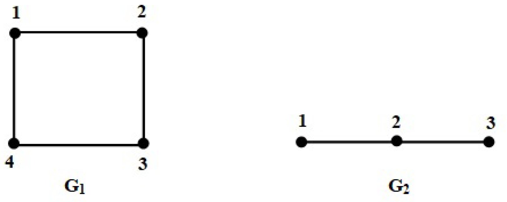
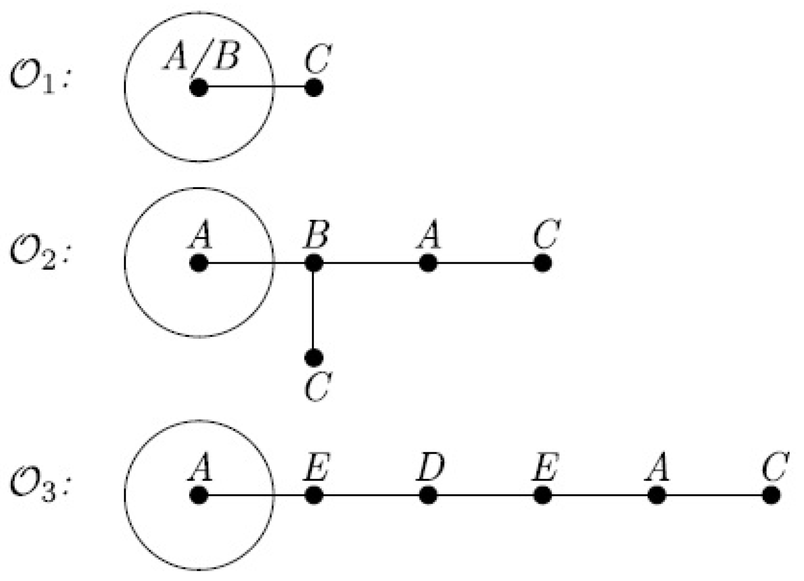
([92]). Let T be a tree, γ${}_{ve}$${}^t$(T) = γ${}^t$(T) if and only if T ∈ $\mathcal{T}$${}_{55}$.

4. Conclusions

Dominating sets are a special topic in graph theory with multiple inputs in various angles by different researchers. In general, one interested in graph theory is also interested characterizing trees using dominating sets. In this article, we have attempted to provide a brief survey of tree characterization using different kinds of dominating sets. In this survey, we observe the following:

• Vertex merging, edge addition and attaching a particular kind of tree are the general graph operations used for building trees.
• In many cases, the initial tree T${}_1$ is either a path or a star graph.
• The most frequently used trees in the iterations are P${}_n$, star and double star trees.

From this survey, we also observe that characterizing trees with equal domination number is also of interest to researchers. This survey provides a collective information of all these for different kinds of dominating sets. This review can help beginners to focus and develop new characterizations in a different dimensions. It would help them to compare the existing operations used for different dominating sets and develop unique set of operations, which we believe would help in characterizing multiple dominating sets, using these set of operations only. The characterizations presented here on trees with equal domination numbers will support them to reason out the possibilities of deciding the equality of domination number between different types of domination even, before developing a new characterization in this view. It would also help them to justify the need to characterize trees with equal domination numbers. It would be useful for them to reason why the particular types of dominating sets are picked for equality characterizations. We believe that this well-summarized review can assist beginner researchers to grasp the concepts and further develop new characterizations.