Article

Advances in Parameter Estimation and Learning from Data for Mathematical Models of Hepatitis C Viral Kinetics

1
Department of Computer Science, Université du Québec à Montréal, Montréal, QC H3C 3P8, Canada
2
Department of Software Engineering, Sami Shamoon College of Engineering, Beer-Sheva 8410802, Israel
3
Program for Experimental and Theoretical Modeling, Division of Hepatology, Department of Medicine, Stritch School of Medicine, Loyola University Chicago, Maywood, IL 60153, USA
4
Department of Computer Science, Ben-Gurion Universty, Beer-Sheva 8410501, Israel
*
Authors to whom correspondence should be addressed.
Mathematics 2022, 10(12), 2136; https://doi.org/10.3390/math10122136
Submission received: 12 April 2022 / Revised: 27 May 2022 / Accepted: 16 June 2022 / Published: 19 June 2022

Abstract

:
Mathematical models, some of which incorporate both intracellular and extracellular hepatitis C viral kinetics, have been advanced in recent years for studying HCV–host dynamics, antivirals mode of action, and their efficacy. The standard ordinary differential equation (ODE) hepatitis C virus (HCV) kinetic model keeps track of uninfected cells, infected cells, and free virus. In multiscale models, a fourth partial differential equation (PDE) accounts for the intracellular viral RNA (vRNA) kinetics in an infected cell. The PDE multiscale model is substantially more difficult to solve compared to the standard ODE model, with governing differential equations that are stiff. In previous contributions, we developed and implemented stable and efficient numerical methods for the multiscale model for both the solution of the model equations and parameter estimation. In this contribution, we perform sensitivity analysis on model parameters to gain insight into important properties and to ensure our numerical methods can be safely used for HCV viral dynamic simulations. Furthermore, we generate in-silico patients using the multiscale models to perform machine learning from the data, which enables us to remove HCV measurements on certain days and still be able to estimate meaningful observations with a sufficiently small error.

1. Introduction

Viral dynamic mathematical models are useful in our understanding of the in vivo kinetics of a variety of viruses that trigger both persistent infection (e.g., HIV-1 [1,2,3,4,5], HBV [6,7,8], HDV [9,10,11,12], Theiler’s encephalomyelitis virus [13], herpes [14] and HCV [15,16,17]) and acute infection (e.g., SARS-CoV-2, influenza A [18] and ebola [19,20]). Mathematical models are also improving our understanding of intracellular viral genome dynamics. The standard model for HCV kinetics during treatment [15] provided helpful insights into the effectiveness and the mechanism of action of interferon-alpha (IFN) as well as ribavirin. The standard model has been applied both retrospectively [21,22] and prospectively, i.e., on treatment [23] to predict the duration of IFN-free antiviral treatment with direct-acting agents (DAAs) [24] needed for HCV eradication (termed time-to-cure). New models were developed to meet the challenges of therapy such as drug resistance [25] and cure after an ultrashort duration of therapy [26]. Notably, age-based multiscale mathematical models for HCV dynamics provided a comprehensive understanding of the nature of viral dynamics patterns observed in patients that were treated with IFN and direct-acting agents such as the HCV protease inhibitors [27], or the HCV NS5A inhibitor daclatasvir [28,29].
The standard model [15] is a set of three ordinary differential equations (ODEs) with three variables: the uninfected target cells (T), the productively infected cells (I), and the free virus in blood (V). Age-structured multiscale models [27,28,30] consider the intercellular viral RNA (vRNA) in an additional equation for the RNA variable (R), by introducing age-dependency in addition to time-dependency, bringing it to a partial differential equation (PDE) model.
We provided a stable and efficient numerical method for multiscale models [31]. Unlike the use of numerical methods in some other applications, for example, in nonlinear diffusion in image processing [32,33] where the accuracy can be limited, here it was advisable to use a stable and efficient scheme belonging to the Runge–Kutta family of numerical schemes with at least a fourth-order of accuracy. Moreover, due to the properties of the model differential equations that are stiff and also an additional integral that is required to be evaluated at every time step, implicit numerical solvers with an adaptive stepsize are significantly more efficient and more stable than the fourth-order Runge–Kutta. Thus, we have chosen to implement an implicit scheme with an adaptive stepsize [34] that is highly efficient and, at the same time, stable for use in multiscale models with the age of HCV dynamics. Furthermore, we provided a suitable method for our numerical work for parameter estimation in [35]. To complement the work in [35], we also wish to address the sensitivity of the parameters in HCV mathematical models by performing a rigorous sensitivity analysis. Finally, we recently used machine learning methods to predict the time for virus elimination from a patient’s extracellular fluid (termed time-to-cure) under DAA therapy in in-silico patients, which were generated by the biphasic model and assessed the accuracy of the predictions [36]. In the current study, we aimed to generate in silico patients by the multiscale model (that predicts more than two phases of viral decline under therapy) and use machine learning methods to estimate time-to-cure and compare them with the predictions of the biphasic model. The multiscale model incorporates possible drug effects on the HCV intracellular lifecycle that the biphasic model does not, namely blocking assembly/secretion, vRNA replication or enhancing vRNA degradation, with the motivation to better understand and simulate the mechanisms that govern the early virologic response to treatment. Being a more sophisticated model, the parameters are more difficult to estimate with the multiscale model relative to the biphasic model [35]. In the following sections, we briefly describe both the biphasic and multiscale models along with their sensitivity analysis and their time-to-cure predictions. We start with the descriptions of the models, continue to their sensitivity analysis, and then we perform learning from data to predict time-to-cure, after which we follow with a discussion of the results that were obtained.

2. The Models Description

2.1. The Biphasic Model

The standard biphasic model for HCV kinetics during treatment [15] is described first. The three variables that this model keeps track of are target cells T, in Equation (1), infected cells I in Equation (2) and free virus V in Equation (3). The target cells T are produced at a constant rate s, die at a per capita rate d and are infected by the virus V at a constant rate β . The infected cells I grow with new infections at a rate β V ( t ) T ( t ) and die at a constant rate δ . The virus V is produced at a rate p by each infected cell. It is cleared at a constant rate c. The ϵ term represents the effectiveness of the treatment, which decreases the production from p to ( 1 ϵ ) p . The system of ODEs for the biphasic model can be written as:
T . ( t ) = s d T ( t ) β V ( t ) T ( t )
I . ( t ) = β V ( t ) T ( t ) δ I ( t )
V . ( t ) = ( 1 ϵ ) p I ( t ) c V ( t ) .
This ODE model is mathematically much simpler as compared to the PDE multiscale model described next. Although the model is nonlinear, it can be solved analytically if we assume that T is constant (i.e., target cells remain constant during antiviral therapy) [15]. The stability analysis of the model was addressed in [37].

2.2. The Multiscale Model

The multiscale model of HCV kinetics [27,28,30] uses the standard biphasic model that considers uninfected target cells in the first equation (Equation (4)), infected cells in the second equation (Equation (5)), and free virus in the third equation (Equation (6)), while also considering vRNA (R) dynamics in an infected cell in the fourth equation (Equation (7). The first three equations comprise the standard biphasic model. The multiscale model is described by:
T . ( t ) = s d T ( t ) β V ( t ) T ( t )
I . ( t ) = β V ( t ) T ( t ) δ I ( t )
V . ( t ) = ( 1 ϵ ) p I ( t ) c V ( t )
R . ( a ) = [ ρ ( a ) + μ ( a ) ] R ( a ) + α ( a ) ,
where in the fourth equation we have also used Newton’s notation for the time derivative, even though the time variable in this equation is not t but the age, a. The four equations can be equivalently formulated in Leibniz’s notation, for simplicity, as follows [28]:
d T ( t ) d t = s d T ( t ) β V ( t ) T ( t )
I ( a , t ) t + I ( a , t ) a = δ ( a ) I ( a , t )
d V ( t ) d t = ( 1 ϵ s ) ρ 0 R ( a , t ) I ( a , t ) d a c V ( t )
R ( a , t ) t + R ( a , t ) a = ( 1 ϵ α ) α ( a ) κ μ ( a ) R ( a , t ) ( 1 ϵ s ) ρ ( a ) R ( a , t ) ,
subject to the auxiliary conditions I ( 0 , t ) = β V ( t ) T ( t ) , I ( a , 0 ) = I ¯ ( a ) , R ( 0 , t ) = 1 , and R ( a , 0 ) = R ¯ ( a ) .
Model parameters of T, in Equation (8), and I, in Equation (9), are similar to the biphasic model. The time variable a is the age of infection and the time variable t is the time duration from therapy initiation. The quantity of free virus V that is shown in Equation (10) depends on the number of the assembled and released virions, as well as their clearance rate c. The quantity of intracellular vRNA R, Equation (11), depends on its synthesis α and degradation μ and its expulsion from the cell ρ . Antiviral treatment blocks the intracellular synthesis of R (parameter ϵ α ) and/or blocks R secretion (parameter ϵ s ), and/or enhances R degradation. The multiscale model has been further investigated and applied in [38,39,40,41].

3. Sensitivity Analysis

To understand the robustness of simulation results obtained when applying the methods of [31,35], we performed a sensitivity analysis on the biphasic and multiscale models. The idea behind the analysis is as follows. We want to track how different parameters affect the outcome of our model, in this case, the number of free virions in the blood after two days. We will generate a large ensemble of well-distributed values over a certain range for each parameter and randomly match them to create a set of randomly initialized parameters. For each of those sets, we then compute our desired outcome. Instead of comparing the raw values, we will compare their rankings. These rank variations determine which parameters are the most influential. In both models, the analysis was performed on the number of free virions in the blood after two days. We followed the protocol described in [42] to evaluate the partial rank correlation coefficient (PRCC) of the different parameters. It is interesting to note that the partial rank correlation coefficient analysis is based on Pearson’s correlation that is used to derive the histogram correlation [43] as employed in [44]. Latin hypercube sampling was performed on 1000 samples, where each parameter was evaluated between half and twice its value. A negative PRCC indicates that an increase in the parameter decreases the number of free virions after two days, while a positive one indicates that it increases it.

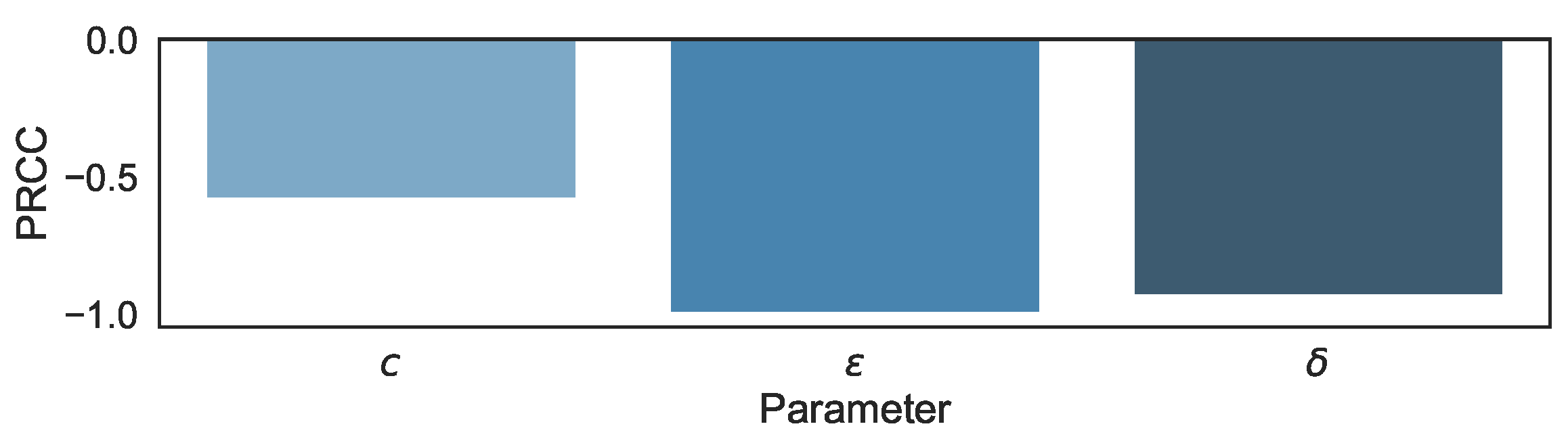
3.1. Sensitivity Analysis in the Biphasic Model

For the biphasic model, three parameters are present: the clearance rate c, the infected-cell loss rate δ and the effectiveness of the blocking of viral production by the treatment ε . Having as an initial value the parameter values that are depicted in Table 1, we performed uniform Latin hypercube sampling in the range 1 / 2 to 2 times those values. The results all had highly significant p-values, below 0.001 and are shown in Figure 1. As expected, they are all negatively correlated with the number of free virions.

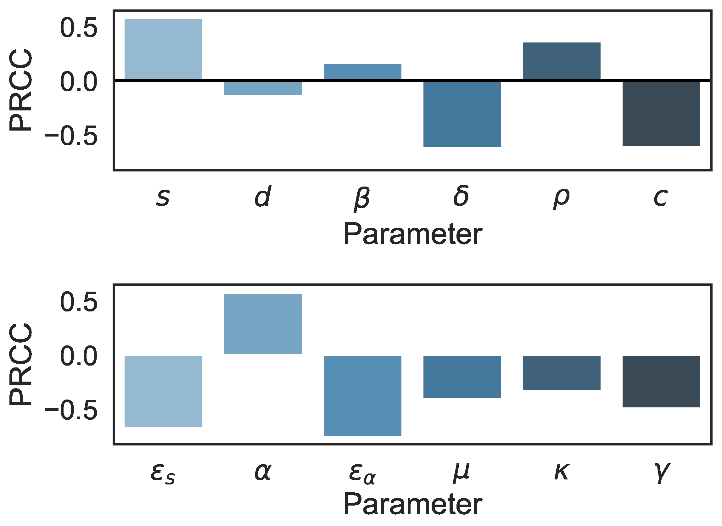
3.2. Sensitivity Analysis in the Multiscale Model
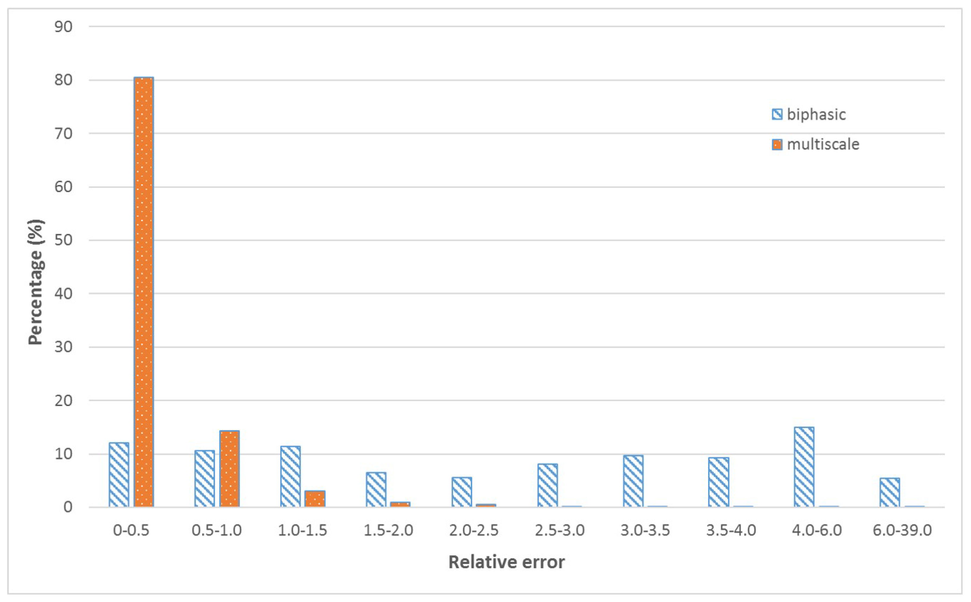
There are twelve parameters in the multiscale model. The central values of each of the parameters are shown in Table 2. All parameters are significantly different from 0 with a p-value below 0.001 .
We observe, as shown in Figure 2, that only four parameters are positively correlated. They are the rate of target cell production s, the new infection rate β , the virus assembly/secretion rate ρ , and the intracellular viral RNA synthesis α . In contrast, the DAA inhibition parameters ε s and ε α , which model the decay of viral replication templates, are negatively correlated as expected.

4. Machine Learning

Parameter estimation uses data information to calibrate the model. The importance of the data can be further exploited by a machine learning approach that was recently presented in [36] in which only the biphasic model was simulated. To compare the utility of machine learning on the biphasic and multiscale models, we generated two datasets of 3000 in-silico patients based on assumed/estimated parameter space in [27,28]. To create the biphasic dataset, the model that was described in [36] was used to generate random parameter values that are uniformly distributed while constrained to the prescribed parameter bounds provided in that reference. To create the multiscale dataset, the model that was described in [35] was used to generate random parameter values that are uniformly distributed while constrained to the following prescribed parameter bounds: β (0.00000005 mL/day/virion), δ (0.14/day), ρ (8.18/day), c (22.3/day), d (0.01/day), α (40.0 vRNA/day), μ (1.0/day), κ (3.5–6.7), γ (0.2–0.96/day), ϵ s (0.4–0.8), ϵ a (0.9–0.999), and s (4.62–6.48 log(cells/mL)). For visualization purposes, the dynamics are depicted in Figure 3 generated using our in-house multiscale model HCV simulator [29] with example trajectories in which the parameter ϵ a was simulated with three parameter values: 0.97, 0.985, and 0.999. In Figure 4, we performed a one-way sensitivity analysis of the multiscale model in predicting time-to-cure. In addition, we provide in Appendix A the figures demonstrating how each one of the parameters that were varied in the one-way sensitivity analysis influence time-to-cure. For each of the generated in silico patients in each dataset, the values for the virus amount during DAA therapy were generated on days 0, 1, 7, 14, 28 (the days at which serum HCV were measured in the proof of concept pilot study [24]). The time-to-cure (defined as one virus copy in the entire extracellular body fluid as used in [24]) was calculated for each patient using the biphasic and multiscale models.
Next, machine learning was applied in order to predict the time-to-cure of the patients in both datasets. This was performed using the freely distributed machine learning Weka software, which is freely available at https://waikato.github.io/weka-wiki/downloading_weka/, accessed on 11 April 2022. Several machine learning methods were tried, including linear regression, support vector machine, neural networks and random-forest. The different classifiers were tested using default parameters, and we found that neural networks provided the best results in all our experiments [45,46,47], which were sufficient for our needs, although it might be possible to reach even better error values if more sophisticated methods such as deep learning were tried.
For checking the efficiency of the machine learning method when applied to each in-silico dataset, we utilized a customary 66–34% framework for the train-test scheme. We trained with data of 66% of the patients (our ‘train’ set) in order to estimate the time-to-cure on untrained data of 34% of the patients (our ‘test’ set). It was faster than 10-fold validation but provided similar errors to when the data set is large.
If we include all HCV measurements (i.e., at 0, 1, 7, 14, and 28 days) in the biphasic and multiscale datasets and use the neural network machine learning regressor for classification, we obtain about 1.7% (biphasic) and 0.65% (multiscale) error on average in predicting the time-to-cure. In Figure 5, the distribution of relative errors obtained for predicting time-to-cure is presented. Opting for an economized protocol in which fewer HCV measurements are used (as theoretically performed in [48]), we removed the days 1 and 7, while remaining only with the days 0, 14, 28. Using only these 3 days, we obtain the distribution of relative errors, as shown in Figure 6. To generate the multiscale results of Figure 5 and Figure 6, it took around 3 days of computing time on a standard PC (Intel(R) Core(TM) i7-7829HQ CPU at 2.90 GHz with 32GB RAM). Furthermore, if we remove days 2 and 28 (not shown in the figures), corroborating [48] specifically, we obtain errors of 3.82% and 1.08%, respectively. It can be observed from these results that the error is about four times less when the multiscale model is used (additionally, one can check Figure 5), which is an even larger ratio than before the removal of days. It can be concluded that for scenarios in which we remove some of the days, the advantage of the multiscale model could reveal itself significantly.

5. Discussion

Two established hepatitis C viral dynamic models have been examined and compared to each other in terms of parameter estimation and learning from data. The first is the classical biphasic model [15], and the second is the multiscale model [27,28]. Before patient data can assist in calibrating the model or estimating important quantities such as time-to-cure, it is worthwhile performing preparatory analyses such as a sensitivity analysis [42] (see Figure 1 and Figure 2) and a machine learning analysis based on simulations with in-silico patients [36] as described in the current study (see Figure 5 and Figure 6).
The sensitivity analysis reveals a safe behavior for the use of numerical methods in both models. The machine learning analysis supports using fewer HCV measurements (compared to five time points used in the pilot study [24]) to predict time-to-cure. This would likely simplify the on-treatment monitoring procedure during DAA treatment along with reducing DAA costs.

Author Contributions

Conceptualization, D.B.; Funding acquisition, H.D. and D.B.; Investigation, V.R., A.C., H.D. and D.B.; Methodology, V.R., A.C., H.D. and D.B.; Project administration, H.D. and D.B.; Software, V.R. and A.C.; Validation, V.R. and A.C.; Visualization, V.R. and A.C.; Writing—original draft, V.R., A.C., H.D. and D.B.; Writing—review & editing, V.R., A.C., H.D. and D.B. All authors have read and agreed to the published version of the manuscript.

Funding

The research was partly supported by the U.S. National Institutes of Health (NIH) grants R01-AI078881, R01-AI158666 and R01-GM121600.

Institutional Review Board Statement

Not applicable.

Informed Consent Statement

Not applicable.

Data Availability Statement

Not applicable.

Conflicts of Interest

The authors declare no conflict of interest.

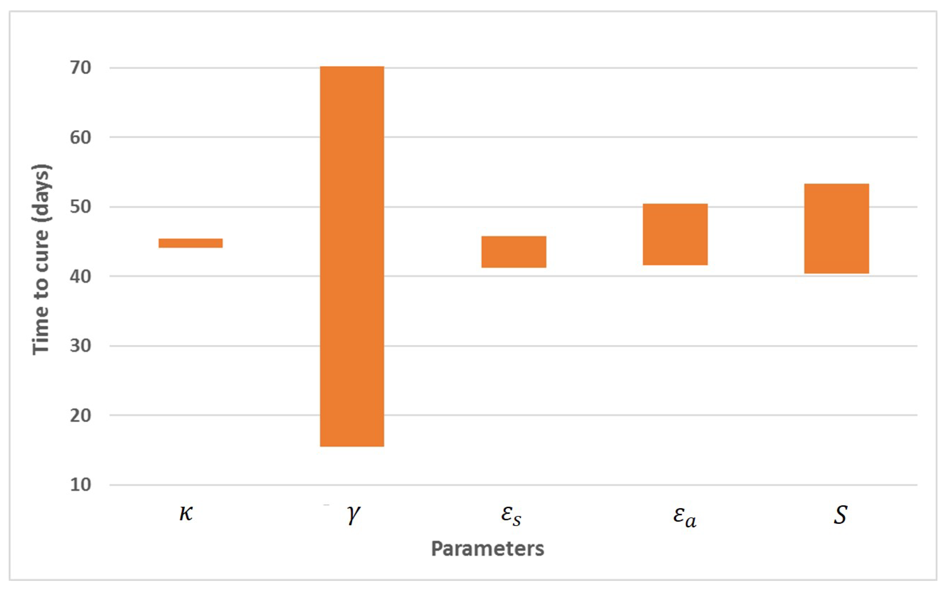
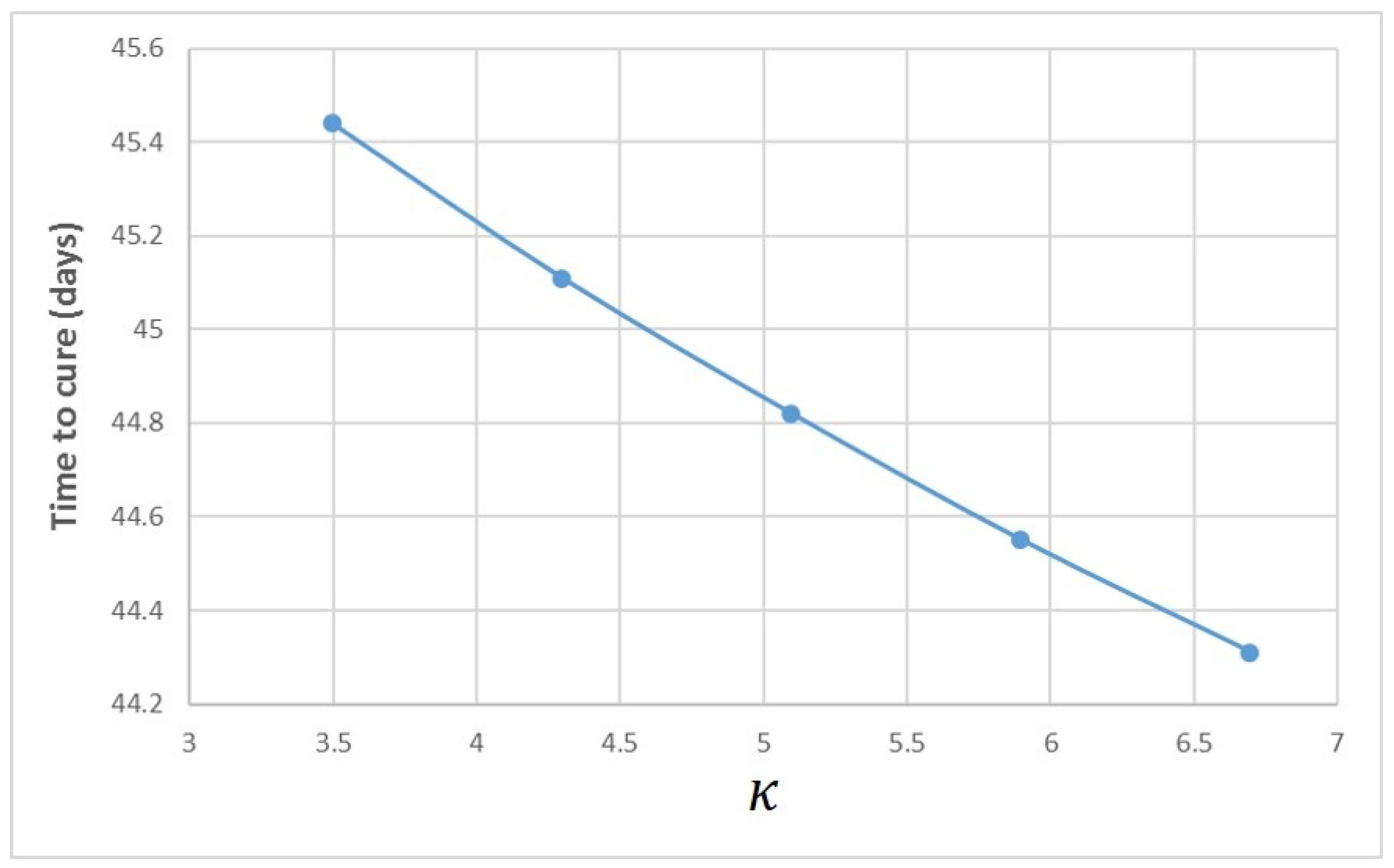
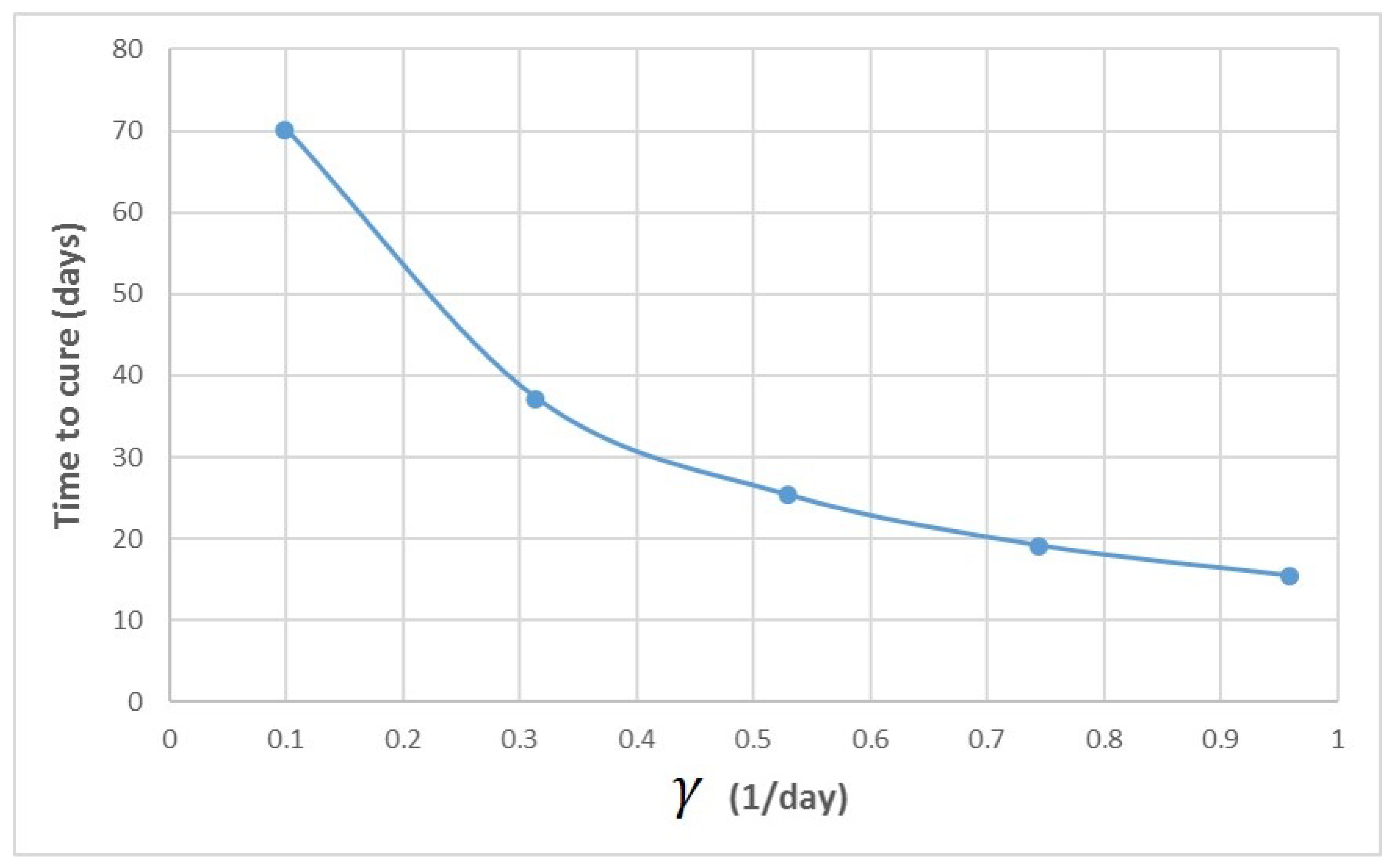
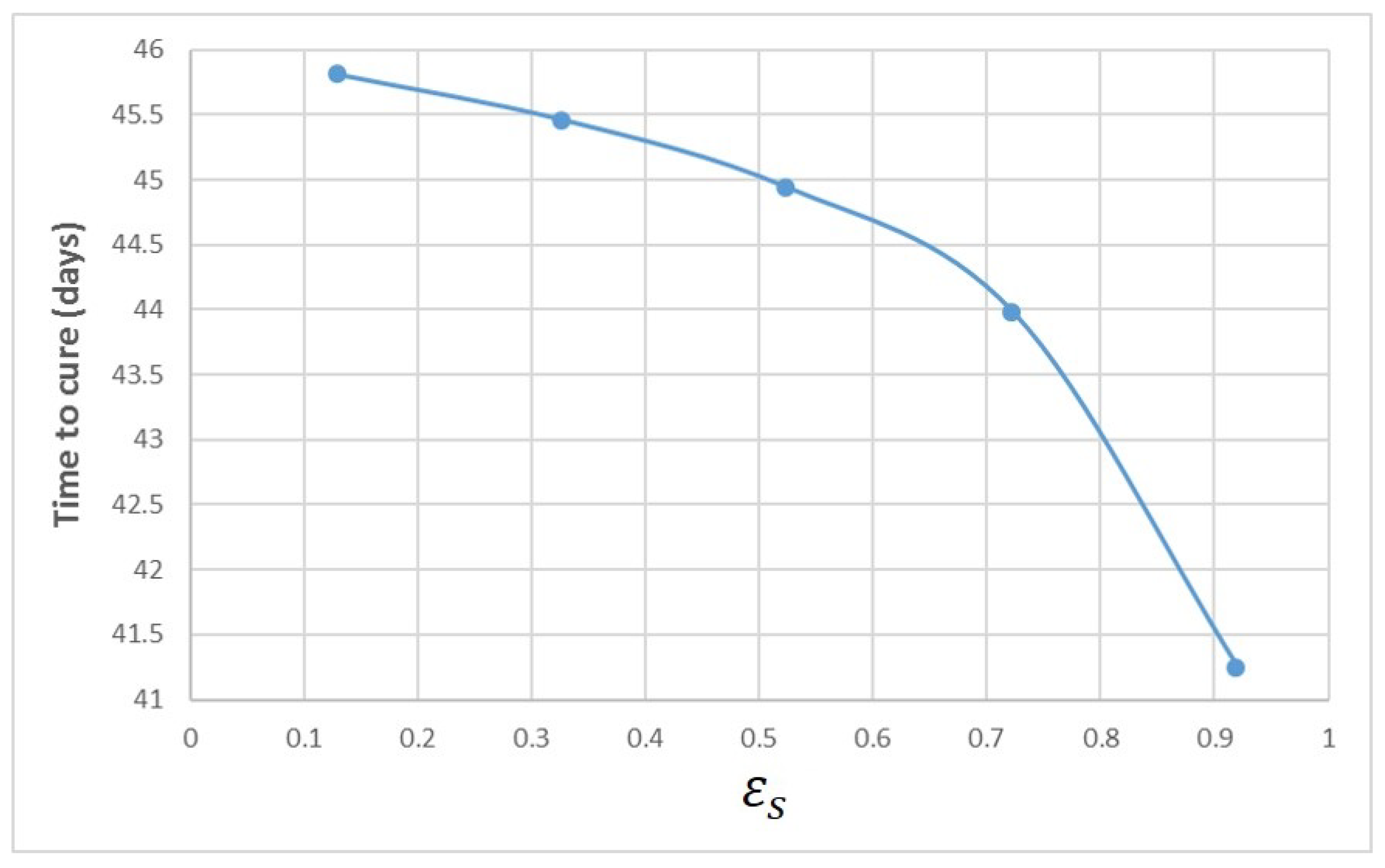
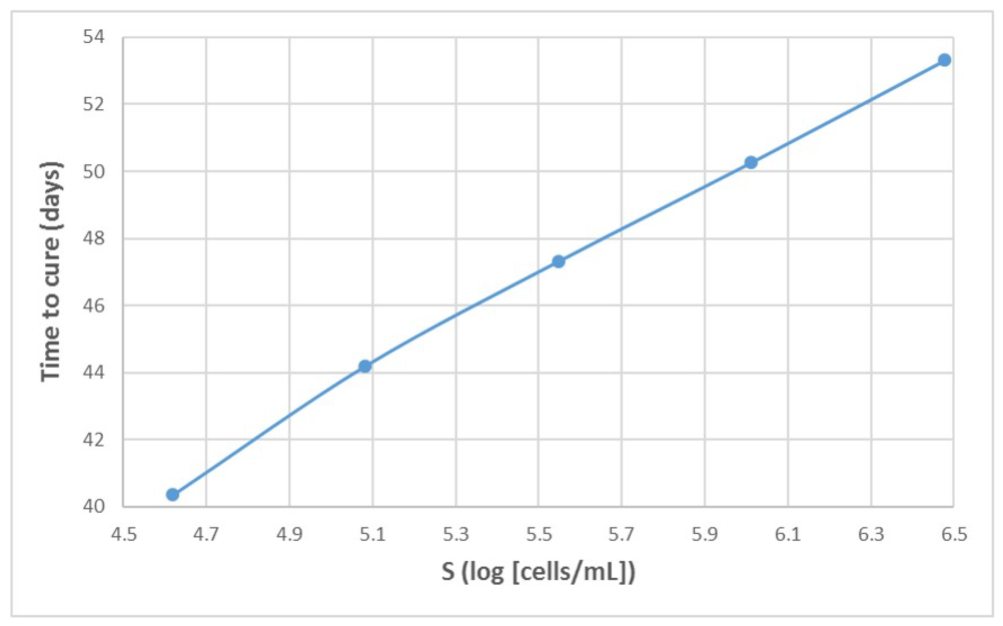
Appendix A. Influence of Multiscale Model Parameters on Time-to-Cure

For each of the varied parameters in the one-way sensitivity analysis shown in Figure 4, we provide a figure that demonstrates how it influences time-to-cure. Depicted is how κ affects time-to-cure in Figure A1, how γ affects time-to-cure in Figure A2, how ϵ s affects time-to-cure in Figure A3, how ϵ a affects time-to-cure in Figure A4, and how s affects time-to-cure in Figure A5. The other parameters were fixed as follows: β (0.00000005 mL/day/virion), δ (0.14/day), ρ (8.18/day), c (22.3/day), d (0.01/day), α (40.0 vRNA/day), and μ (1.0/day).
Figure A1. Influence of parameter κ in the multiscale model on time-to-cure.
Mathematics 10 02136 g0a1
Figure A2. Influence of parameter γ in the multiscale model on time-to-cure.
Mathematics 10 02136 g0a2
Figure A3. Influence of parameter ϵ s in the multiscale model on time-to-cure.
Mathematics 10 02136 g0a3
Figure A4. Influence of parameter ϵ a in the multiscale model on time-to-cure.
Mathematics 10 02136 g0a4
Figure A5. Influence of parameter s in the multiscale model on time-to-cure.
Mathematics 10 02136 g0a5

References

  1. Perelson, A.S. Modelling viral and immune system dynamics. Nat. Rev. Immunol. 2002, 2, 28–36. [Google Scholar] [CrossRef] [PubMed]
  2. Ho, D.D.; Neumann, A.U.; Perelson, A.S.; Chen, W.; Leonard, J.M.; Markowitz, M. Rapid turnover of plasma virions and CD4 lymphocytes in HIV-1 infection. Nature 1995, 373, 123. [Google Scholar] [CrossRef] [PubMed]
  3. Perelson, A.S.; Neumann, A.U.; Markowitz, M.; Leonard, J.M.; Ho, D.D. HIV-1 dynamics in vivo: Virion clearance rate, infected cell life-span, and viral generation time. Science 1996, 271, 1582. [Google Scholar] [CrossRef] [PubMed] [Green Version]
  4. Burg, D.; Rong, L.; Neumann, A.U.; Dahari, H. Mathematical modeling of viral kinetics under immune control during primary HIV-1 infection. J. Theor. Biol. 2009, 259, 751–759. [Google Scholar] [CrossRef] [PubMed]
  5. Aviran, A.; Shah, P.S.; Schaffer, D.P.; Arkin, P.A. Computational Models of HIV-1 Resistance to Gene Therapy Elucidate Therapy Design Principles. PLoS Comput. Biol. 2010, 6, e1000883. [Google Scholar] [CrossRef]
  6. Ciupe, S.M.; Ribeiro, R.M.; Nelson, P.W.; Dusheiko, G.; Perelson, A.S. The role of cells refractory to productive infection in acute hepatitis B viral dynamics. Proc. Natl. Acad. Sci. USA 2007, 104, 5050–5055. [Google Scholar] [CrossRef] [Green Version]
  7. Ribeiro, R.M.; Germanidis, G.; Powers, K.A.; Pellegrin, B.; Nikolaidis, P.; Perelson, A.S.; Pawlotsky, J.M. Hepatitis B Virus Kinetics under Therapy Sheds Light on Differences Between e-antigen Positive and Negative Infection. J. Infect. Dis. 2010, 202, 1309–1318. [Google Scholar] [CrossRef]
  8. Nowak, M.A.; Bonhoeffer, S.; Hill, A.M.; Boehme, R.; Thomas, H.C.; McDade, H. Viral dynamics in hepatitis B virus infection. Proc. Natl. Acad. Sci. USA 1996, 93, 4398–4402. [Google Scholar] [CrossRef] [Green Version]
  9. Koh, C.; Canini, L.; Dahari, H.; Zhao, X.; Uprichard, S.L.; Haynes-Williams, V.; Winters, M.A.; Subramanya, G.; Cooper, S.L.; Pinto, P.; et al. Oral prenylation inhibition with lonafarnib in chronic hepatitis D infection: A proof-of-concept randomised, double-blind, placebo-controlled phase 2A trial. Lancet Infect. Dis. 2015, 15, 1167–1174. [Google Scholar] [CrossRef] [Green Version]
  10. Guedj, J.; Rotman, Y.; Cotler, S.J.; Koh, C.; Schmid, P.; Albrecht, J.; Haynes-Williams, V.; Liang, T.J.; Hoofnagle, J.H.; Heller, T.; et al. Understanding early serum hepatitis D virus and hepatitis B surface antigen kinetics during pegylated interferon-alpha therapy via mathematical modeling. Hepatology 2014, 60, 1902–1910. [Google Scholar] [CrossRef]
  11. Shekhtman, L.; Cotler, S.J.; Hershkovich, L.; Uprichard, S.L.; Bazinet, M.; Pantea, V.; Cebotarescu, V.; Cojuhari, L.; Jimbei, P.; Krawczyk, A.; et al. Modelling hepatitis D virus RNA and HBsAg dynamics during nucleic acid polymer monotherapy suggest rapid turnover of HBsAg. Sci. Rep. 2020, 10, 7837. [Google Scholar] [CrossRef] [PubMed]
  12. Shekhtman, L.; Cotler, S.J.; Ploss, A.; Dahari, H. Mathematical modeling suggests that entry-inhibitor bulevirtide may interfere with hepatitis D virus clearance from circulation. J. Hepatol. 2022, 76, 1229–1231. [Google Scholar] [CrossRef] [PubMed]
  13. Zhang, J.; Lipton, H.L.; Perelson, A.S.; Dahari, H. Modeling the acute and chronic phases of Theiler murine encephalomyelitis virus infection. J. Virol. 2013, 87, 4052–4059. [Google Scholar] [CrossRef] [PubMed] [Green Version]
  14. Schiffer, J.T.; Abu-Raddad, L.; Mark, K.E.; Zhu, J.; Selke, S.; Magaret, A.; Wald, A.; Corey, L. Frequent release of low amounts of herpes simplex virus from neurons: Results of a mathematical model. Sci. Transl. Med. 2009, 1, 7ra16. [Google Scholar] [CrossRef] [PubMed] [Green Version]
  15. Neumann, A.U.; Lam, N.P.; Dahari, H.; Gretch, D.R.; Wiley, T.E.; Layden, T.J.; Perelson, A.S. Hepatitis C viral dynamics in vivo and the antiviral efficacy of interferon-α therapy. Science 1998, 282, 103–107. [Google Scholar] [CrossRef]
  16. Shekhtman, L.; Navasa, M.; Sansone, N.; Crespo, G.; Subramanya, G.; Chung, T.L.; Cardozo-Ojeda, E.F.; Pérez-del Pulgar, S.; Perelson, A.S.; Cotler, S.J.; et al. Modeling hepatitis C virus kinetics during liver transplantation reveals the role of the liver in virus clearance. Elife 2021, 10, e65297. [Google Scholar] [CrossRef]
  17. Wasik, S.; Jackowiak, P.; Figlerowicz, M.; Blazewicz, J. Multi-agent model of hepatitis C virus infection. Artif. Intell. Med. 2014, 60, 123–131. [Google Scholar] [CrossRef] [Green Version]
  18. Boianelli, A.; Nguyen, V.K.; Ebensen, T.; Schulze, K.; Wilk, E.; Sharma, N.; Stegemann-Koniszewski, S.; Bruder, D.; Toapanta, F.R.; Guzmán, C.A.; et al. Modeling influenza virus infection: A roadmap for influenza research. Viruses 2015, 7, 5274–5304. [Google Scholar] [CrossRef] [Green Version]
  19. Madelain, V.; Oestereich, L.; Graw, F.; Nguyen, T.H.T.; De Lamballerie, X.; Mentré, F.; Günther, S.; Guedj, J. Ebola virus dynamics in mice treated with favipiravir. Antivir. Res. 2015, 123, 70–77. [Google Scholar] [CrossRef] [Green Version]
  20. Chertow, D.S.; Shekhtman, L.; Lurie, Y.; Davey, R.T.; Heller, T.; Dahari, H. Modeling challenges of Ebola virus–host dynamics during infection and treatment. Viruses 2020, 12, 106. [Google Scholar] [CrossRef] [Green Version]
  21. Dahari, H.; Canini, L.; Graw, F.; Uprichard, S.L.; Araujo, E.S.A.; Penaranda, G.; Coquet, E.; Chiche, L.; Riso, A.; Renou, C.; et al. HCV kinetic and modeling analyses indicate similar time to cure among sofosbuvir combination regimens with daclatasvir, simeprevir or ledipasvir. J. Hepatol. 2016, 54, 1232–1239. [Google Scholar] [CrossRef] [PubMed] [Green Version]
  22. Dasgupta, S.; Imamura, M.; Gorstein, E.; Nakahara, T.; Tsuge, M.; Churkin, A.; Yardeni, D.; Etzion, O.; Uprichard, S.L.; Barash, D.; et al. Modeling-Based Response-Guided Glecaprevir-Pibrentasvir Therapy for Chronic Hepatitis C to Identify Patients for Ultrashort Treatment Duration. J. Infect. Dis. 2020, 222, 1165–1169. [Google Scholar] [CrossRef] [PubMed]
  23. Dahari, H.; Shteingart, S.; Gafanovich, I.; Cotler, S.J.; D’Amato, M.; Pohl, R.T.; Weiss, G.; Ashkenazi, Y.J.; Tichler, T.; Goldin, E.; et al. Sustained virological response with intravenous silibinin: Individualized IFN-free therapy via real-time modelling of HCV kinetics. Liver Int. 2015, 35, 289–294. [Google Scholar] [CrossRef] [PubMed] [Green Version]
  24. Etzion, O.; Dahari, H.; Yardeni, D.; Issachar, A.; Nevo-Shor, A.; Cohen-Naftaly, M.; Ashur, Y.; Uprichard, S.L.; Sneh Arbib, O.; Munteanu, D.; et al. Response guided therapy for reducing duration of direct acting antivirals in chronic hepatitis C infected patients: A Pilot study. Sci. Rep. 2020, 10, 17820. [Google Scholar] [CrossRef] [PubMed]
  25. Rong, L.; Dahari, H.; Ribeiro, R.M.; Perelson, A.S. Rapid emergence of protease inhibitor resistance in hepatitis C virus. Sci. Transl. Med. 2010, 2, 30ra32. [Google Scholar] [CrossRef] [PubMed] [Green Version]
  26. Goyal, A.; Lurie, Y.; Meissner, G.; Major, M.; Sansone, N.; Uprichard, S.; Cotler, S.; Dahari, H. Modeling HCV cure after an ultra-short duration of therapy with direct acting agents. Antivir. Res. 2017, 30, 281–285. [Google Scholar] [CrossRef]
  27. Rong, L.; Guedj, J.; Dahari, H.; Coffield, D.J.J.; Levi, M.; Smith, P.; Perelson, A.S. Analysis of hepatitis C virus decline during treatment with the protease inhibitor danoprevir using a multiscale model. PLoS Comput. Biol. 2013, 9, e1002959. [Google Scholar] [CrossRef]
  28. Guedj, J.; Dahari, H.; Rong, L.; Sansone, N.D.; Nettles, R.E.; Cotler, S.J.; Layden, T.J.; Uprichard, S.L.; Perelson, A.S. Modeling shows that the NS5A inhibitor daclatasvir has two modes of action and yields a shorter estimate of the hepatitis C virus half-life. Proc. Natl. Acad. Sci. USA 2013, 110, 3991–3996. [Google Scholar] [CrossRef] [Green Version]
  29. Reinharz, V.; Churkin, S.; Dahari, H.; Barash, D. A Robust and Efficient Numerical Method for RNA-Mediated Viral Dynamics. Front. Appl. Math. Stat. 2017, 3, 20. [Google Scholar] [CrossRef] [Green Version]
  30. Rong, L.; Perelson, A.S. Mathematical analysis of multiscale models for hepatitis C virus dynamics under therapy with direct-acting antiviral agents. Math. Biosci. 2013, 245, 22–30. [Google Scholar] [CrossRef] [Green Version]
  31. Reinharz, V.; Dahari, H.; Barash, D. Numerical schemes for solving and optimizing multiscale models with age of hepatitis C Virus Dynamics. Math. Biosci. 2018, 300, 1–13. [Google Scholar] [CrossRef] [PubMed]
  32. Weickert, J.; Romeny, B.T.H.; Viergever, M. Efficient and reliable schemes for nonlinear diffusion filtering. IEEE Trans. Imag. Proc. 1998, 7, 398–410. [Google Scholar] [CrossRef] [PubMed] [Green Version]
  33. Barash, D. Nonlinear Diffusion Filtering on Extended Neighborhood. Appl. Num. Math. 2005, 52, 1–11. [Google Scholar] [CrossRef]
  34. Rosenbrock, H. Some general implicit processes for the numerical solution of differential equations. Comput. J. 1963, 5, 329–330. [Google Scholar] [CrossRef] [Green Version]
  35. Reinharz, V.; Churkin, A.; Lewkiewicz, S.; Dahari, H.; Barash, D. A Parameter Estimation Method for Multiscale Models of hepatitis C Virus Dynamics. Bull. Math. Biol. 2019, 81, 3675–3721. [Google Scholar] [CrossRef] [PubMed]
  36. Churkin, A.; Kriss, S.; Uziel, A.; Goyal, R.; Zakh, R.; Cotler, S.J.; Etzion, O.; Shlomai, A.; Rotstein, H.G.; Dahari, H.; et al. Machine Learning for Mathematical Models of HCV Kinetics During Antiviral Therapy. Math. Biosci. 2022, 343, 108756. [Google Scholar] [CrossRef]
  37. Dahari, H.; Lo, A.; Ribeiro, R.M.; Perelson, A.S. Modeling hepatitis C virus dynamics: Liver regeneration and critical drug efficacy. J. Theor. Biol. 2007, 247, 371–381. [Google Scholar] [CrossRef] [Green Version]
  38. Quintela, B.; Conway, J.; Hyman, J.; Reis, R.; dos Santos, R.; Lobosco, M.; Perelson, A. An Age-based Multiscale Mathematical Model of the Hepatitis C Virus Life-cycle during Infection and Therapy: Including Translation and Replication. In Proceedings of the VII Latin American Congress on Biomedical Engineering CLAIB 2016, Bucaramanga, Colombia, 26–28 October 2016; Springer: Berlin/Heidelberg, Germany, 2017; pp. 508–511. [Google Scholar]
  39. Kitagawa, K.; Nakaoka, S.; Asai, Y.; Watashi, K.; Iwami, S. A PDE Multiscale Model of hepatitis C virus infection can be transformed to a system of ODEs. J. Theor. Biol. 2018, 267, 330–340. [Google Scholar] [CrossRef]
  40. Kitagawa, K.; Kuniya, T.; Nakaoka, S.; Asai, Y.; Watashi, K.; Iwami, S. Mathematical analysis of a transformed ODE from a PDE multiscale model of hepatitis C virus infection. Bull. Math. Biol. 2019, 81, 1427–1441. [Google Scholar] [CrossRef]
  41. Goncalves, A.; Lemenuel-Diot, A.; Cosson, V.; Jin, Y.; Feng, S.; Bo, Q.; Guedj, J. What drives the dynamics of HBV RNA during treatment? J. Viral Hepat. 2021, 28, 383–392. [Google Scholar] [CrossRef]
  42. Marino, S.; Hogue, I.B.; Ray, C.J.; Kirschner, D.E. A methodology for performing global uncertainty and sensitivity analysis in systems biology. J. Theor. Biol. 2008, 254, 178–196. [Google Scholar] [CrossRef] [PubMed] [Green Version]
  43. Bazan, E.; Dokladal, P.; Dokladalova, E. Quantitative Analysis of Similarity Measures and Distributions. In Proceedings of the 30th British Machine Vision Conference, Cardiff, UK, 9–12 September 2019. [Google Scholar]
  44. Ivry, T.; Michal, S.; Avihoo, A.; Sapiro, G.; Barash, D. An Image Processing Approach to Computing Distances Between RNA Secondary Structures Dot Plots. Algorithms Mol. Biol. 2009, 4, 4. [Google Scholar] [CrossRef] [PubMed] [Green Version]
  45. Haykin, S. Neural Networks: A Comprehensive Foundation, 2nd ed.; Prentice Hall PTR: Hoboken, NJ, USA, 1998. [Google Scholar]
  46. Witten, I.H.; Frank, E.; Hall, M.A.; Pall, C.J. Data Mining: Practical Machine Learning Tools and Techniques, 3rd ed.; Morgan Kaufmann: Burlington, MA, USA, 2011. [Google Scholar]
  47. Strang, G. Linear Algebra and Learning from Data, 1st ed.; Wellesley-Cambridge Press: Wellesley, MA, USA, 2019. [Google Scholar]
  48. Goyal, A.; Churkin, A.; Barash, D.; Cotler, S.J.; Shlomai, A.; Etzion, O.; Dahari, H. Modeling-Based Response-Guided DAA Therapy for Chronic Hepatitis C to Identify Individuals for Shortening Treatment Duration. Open Forum Infec. Dis. 2022, 9, ofac157. [Google Scholar] [CrossRef] [PubMed]
Figure 1. Partial rank correlation coefficient (PRCC) results in the biphasic model.
Mathematics 10 02136 g001
Figure 2. PRCC results of the multiscale model.
Mathematics 10 02136 g002
Figure 3. For visualization purposes, the dynamics with example trajectories in which the parameter ϵ a was simulated with 3 parameter values 0.97, 0.985, and 0.999 is displayed using our in-house multiscale model HCV simulator [29]. The other parameters were fixed as follows: β (0.00000005 mL/day/virion), δ (0.14/day), ρ (8.18/day), c (22.3/day), d (0.01/day), α (40.0 vRNA/day), μ (1.0/day), κ (6.36), γ (0.24/day), ϵ s (0.65), and s (130,000 (cells/mL)).
Mathematics 10 02136 g003
Figure 4. One-way sensitivity analysis of time-to-cure using the multiscale model. Depicted are minimum and maximum time-to-cure values for each parameter that were varied in a defined range (i.e., κ (3.5–6.7), γ (0.2–0.96/day), ϵ s (0.4–0.8), ϵ a (0.9–0.999), and s (4.62–6.48 log(cells/mL)), while the other parameters were fixed as follows: β (0.00000005 mL/day/virion), δ (0.14/day), ρ (8.18/day), c (22.3/day), d (0.01/day), α (40.0 vRNA/day), and μ (1.0/day).
Mathematics 10 02136 g004
Figure 5. Distribution of relative errors obtained for predicting time-to-cure using machine learning with the biphasic and multiscale models. Measurements of all time points (0, 2, 7, 14 and 28 days) were used for the machine learning.
Mathematics 10 02136 g005
Figure 6. Distribution of relative errors obtained for predicting time-to-cure using machine learning with the biphasic and multiscale models. Measurements of reduced time points (0, 14 and 28 days) were used for the machine learning.
Mathematics 10 02136 g006
Table 1. Central values of the biphasic model for the PRCC. The (min, max) of the parameter space are shown.
c ε δ
6.0 ( 3 , 12 ) 0.5 ( 0.25 , 1 ) 0.5 ( 0.25 , 1 )
Table 2. Central values of the multiscale model for the PRCC. The (min, max) of the parameter space are shown.
sd β δ ρ c
130,000 (65,000, 260,000) 0.01 ( 0.05 , 0.02 ) 5   ×   10 8 ( 0.55   ×   10 8 , 25   ×   10 8 ) 0.14 ( 0.07 , 0.28 ) 7.95 ( 3.975 , 15.9 ) 22.5 ( 11.25 , 25 )
ε s α ε α κ μ γ
0.5 ( 0.25 , 1 ) 40 ( 20 , 80 ) 0.5 ( 0.25 , 1 ) 6.36 ( 3.18 , 12.72 ) 1 ( 0.5 , 2 ) 0.24 ( 0.12 , 48 )
Publisher’s Note: MDPI stays neutral with regard to jurisdictional claims in published maps and institutional affiliations.

