Article

Regional Location Routing Problem for Waste Collection Using Hybrid Genetic Algorithm-Simulated Annealing

1
Department of Industrial Management, National Taiwan University of Science and Technology, Taipei 106335, Taiwan
2
Center for Cyber-Physical System Innovation, National Taiwan University of Science and Technology, Taipei 106335, Taiwan
3
Department of Mechanical Engineering, Institut Teknologi Sepuluh Nopember, Surabaya 60111, Indonesia
4
Department of Information Management, Chang Gung University, Taoyuan 33302, Taiwan
5
Department of Industrial Engineering and Management, Ming Chi University of Technology, New Taipei 243303, Taiwan
6
Department of Emergency Medicine, Keelung Chang Gung Memorial Hospital, Keelung 20401, Taiwan
*
Author to whom correspondence should be addressed.
Mathematics 2022, 10(12), 2131; https://doi.org/10.3390/math10122131
Submission received: 19 April 2022 / Revised: 3 June 2022 / Accepted: 10 June 2022 / Published: 19 June 2022
(This article belongs to the Section Engineering Mathematics)

Abstract

:
Municipal waste management has become a challenging issue with the rise in urban populations and changes in people’s habits, particularly in developing countries. Moreover, government policy plays an important role associated with municipal waste management. Thus, this research proposes the regional location routing problem (RLRP) model and multi-depot regional location routing problem (MRLRP) model, which are extensions of the location routing problem (LRP), to provide a better municipal waste collection process. The model is constructed to cover the minimum number of depot facilities’ policy requirements for each region due to government policy, i.e., the large-scale social restrictions in each region. The goal is to determine the depot locations in each region and the vehicles’ routes for collecting waste to fulfill inter-regional independent needs at a minimum total cost. This research conducts numerical examples with actual data to illustrate the model and implements a hybrid genetic algorithm and simulated annealing optimization to solve the problem. The results show that the proposed method efficiently solves the RLRP and MRLRP.

1. Introduction

Municipal waste management is a challenging problem faced by developing countries. This research focuses on handling waste collection due to government policy, i.e., the large-scale social restrictions (LSR). We look to build a scenario approach to provide alternative solutions for the waste collection process. Although the mobility of the population from one area to another is limited, our proposed scenarios are designed to make each region able to solve its waste problems. First, we modify the centralized system into a decentralized one by implementing regional consideration. Therefore, we can reduce the total volume of waste that the final depot must process, shorten the vehicle travel route, and reduce the waste collection time. As a result, each region can handle the waste collection and reduce the volume of waste. Moreover, the route distance for each vehicle falls by opening an alternative depot in each area.
Previous research has shown that regional consideration, such as territory design for last-mile delivery and logistic distribution, contributes to increasing the system’s efficiency [1]. Most service providers avoid optimizing their delivery or pick-up routes each day from scratch for the current customer set. They prefer to partition the territory serviced by a depot into smaller districts that remain constant for a longer time [1]. As a result, each district’s repeated route pattern services make it easier for the drivers according to their own knowledge—for example, a two-stage optimization for the vehicle routing problem where customers have to be divided into regions first and delivery tours within each district must be determined afterward [2]. Carlsson [3] studied an incapacitated version, where customer locations are stochastic but assumed to be distributed according to a known probability density function. Lei et al. [4] subdivided a territory into regions, whereby, over multiple periods with varying deterministic customer sets, multiple traveling salesman problems from multiple depots within each region are minimized.
Although the existing studies have made significant progress in implementing regional considerations into the routing model, most of them mainly focus on an operational decision, such as determining the vehicle routes. Based on the literature, it is proven that this integration will significantly minimize the cost and maximize the service level [5]. One of the integrated approaches is the well-known location-routing problem (LRP).
The LRP literature has been increasing over the years. It covers many real case studies, such as agriculture, airlines, automotive logistics, city logistics, military, e-commerce, disaster management, food distribution, healthcare logistics, oil and energy, postal delivery, telecommunications, and waste management [6]. Each area presents unique challenges for the researchers in their efforts to develop and represent the actual situation. The application of LRP models to optimize a case of waste management is by far the most popular study. Hence, we aim to implement a location routing problem (LRP) model to solve the problem of a waste management system implementing regional factors.
In this study, we consider a regional strategy in waste collection. By doing so, we integrate strategic and operational decisions and a regional constraint. We develop an LRP model that considers the present depot location and new depot alternatives required to be established in each region or district. The model can also determine the route for each vehicle in collecting waste in each district. The study also considers the minimum requirement of depots in each district.
As far as the literature review, this study is the first to examine the minimum number of depots in each area. Moreover, the scenario for the LRP application is implemented to provide alternative solutions during LSR, which is still limited. We develop two models representing two scenarios based on the original LRP model: the regional location routing problem (RLRP) and multi-depot regional location routing problem (MRLPR).
Since the LRP is NP-hard [7] and the RLRP and MRLRP are particular cases of the LRP, then the RLRP and MRLRP are also NP-hard. Thus, using the classical approaches will be challenging because they require a high computational time [8]. Consequently, we propose a metaheuristics approach to solve the model: a hybrid genetic algorithm and simulated annealing (GASA). Compared with other methods, the algorithm provides a competitive solution based on the experiment conducted, such as the Gurobi solver.
Our main contributions are as follows:
  • We present a new location routing problem to solve the waste collection problem and provide some scenarios.
  • We develop a hybrid genetic algorithm and simulated annealing (GASA) that can efficiently solve the model for each scenario.
  • We implement the proposed methods into a real example adopted from PD Kebersihan in Bandung City to provide a more realistic illustration of this waste collection problem
In the remainder of this study, Section 2 presents the relevant literature. Section 3 clearly describes the scenario’s model and application. Section 4 details the solution methodology. Section 5 offers the experimental results and discussion, including the case study regarding PD Kebersihan. Finally, Section 6 provides a conclusion and suggestions for future research.

2. Literature Review

The problem involving operational decisions (routing problem) and strategic decisions (depot location) is known as the location routing problem (LRP) [6]. A general illustration of the LRP can be seen in Appendix A. The LRP model determines the location of facilities (depot, distribution center, or warehouse) and the vehicle’s route simultaneously when delivering goods to the customer(s). The LRP has proven to reduce costs over the long-term of operations and plays a significant role in cost-savings, increased productivity, and delivering positive impacts for operators and communities when they address issues earlier in the long-term planning stages [9].
Since the LRP provides enormous benefits for industries, research on it has evolved with various approaches. The model may use different frameworks reliant on the institution or firm’s judgment, problem assumptions, and factors considered by the decision-makers. Several LRP models have been utilized in different industries, such as in the food and beverage distribution (United Kingdom), the distribution of newspapers (Denmark), rubber plant industries (Malaysia), the garbage collection process (Belgium), billing deliveries (Hong Kong), optical network design (South Korea), and a telecom network (France) [6]. By looking at the applications of the LRP model, we implement the LRP research in different fields.
Many LRP variants now exist. The recent survey paper conducted by Mara et al. [6] shows the classification of research in the LRP field. We categorize LRP models based on type of study, solution approach, scenario characteristics, physical characteristics, and objective function [6]. The type of study includes literature survey, development of theory, research article, and case study. The solution approach includes both exact and approximation methods (classical heuristics, metaheuristics, and simulation). The scenario characteristics relate to the strategic and tactical decisions of the developed model, such as planning period, customer type, and data obtained. On the other hand, the physical characteristics relate to a strategic and operational decision, such as the location of facilities, echelon type, routing type, vehicle type, and capacity consideration. Lastly, the objective function could be classified into cost minimization, environmental aspects, equity distribution, and specific performance indicators.
The location routing problem (LRP) itself was newly developed initially from the vehicle routing problem (VRP) and the facility location problem (FLP) [7]. Since these two problems are included in NP-hard problems, then the LRP is also NP-hard [10]. At least four solution approaches are implemented to solve the LRP model: exact methods, classical heuristics, metaheuristics, and simulation. Based on the recent literature, the metaheuristics method is the most popular one used by researchers from 2014 to 2019 [6]. Metaheuristics is formally defined as an iterative process that guides a subordinate heuristic by combining intelligently different concepts to explore and exploit the search space or create a balance between the intensification and diversification of the search space [11]. The metaheuristic methods that are used to solve the LRP include simulated annealing (SA) [10], genetic algorithm (GA) [12], non-dominated sorting genetic algorithm II (NSGA-II) [13], particle swarm optimization (PSO) [14], ant colony [15], tabu search (TS) [16], large neighborhood search (LNS) [17], iterated local search (ILS) [18], memetic algorithm (MA) [19], differential evolution [20], harmony search [21], hyper-heuristic (HH) [22], cross-entropy algorithm (CEA) [23], and greedy randomized adaptive search procedure (GRASP) [24].
Metaheuristic approaches in finding solutions to routing problems, i.e., the LRP, can generally be grouped into two types, namely (1) single-solution approaches, e.g., SA, TS, ILS, and VNS, and (2) population-based approaches, e.g., GA and PSO [25]. Single solution approaches focus on modifying and improving a candidate solution to meet the evaluation criteria. The current solution will be replaced until a satisfactory result (good-quality solution) is obtained. In contrast, population-based approaches iterate, maintain, and improve multiple candidate solutions, often using population characteristics to guide the search. Both of these solution search processes have advantages and disadvantages.
Single-solution approaches have the advantage of providing better results in terms of quality because of emphasizing an exploitation strategy or focusing on finding optimum solutions around a good (near-)optimal solution [26]. However, the global optimum may not reach and may get stuck in the local optimum due to the randomized initial solution [27]. In contrast, the population-based approach maintains the diversity of the solution globally and has the potency of expanding the search space or exploration strategy, so it has advantages to better search space [26,27]. However, the population-based approach requires sufficient knowledge regarding the search space in the initial steps, so the solution quality may be worse than a single solution because more exploitation is required by a lapse of steps [26]. Therefore, an appropriate trade-off between the single-solution and population-based approaches is necessary for an efficient search.
This research implements a hybrid GA and SA to produce solutions by pursuing a balanced exploitation and exploration strategy. By implementing GA as an initial exploration strategy in the hybrid process, we could avoid trapping into the local optima and increasing the search space. Moreover, GA has an advantage in providing faster computational time, but it is not easy to obtain the optimum value, so we increase the population for GA. In contrast, SA may take a longer computational process since the initial solution is randomized [28]. Therefore, the GA outputs are upgraded using SA to exploit and produce a better solution. Implementing this mechanism could obtain a good solution, as shown in the various types of routing-like problems [29,30,31].
The exact method is the second most preferred choice. Most studies consider the exact method by using commercial solvers, such as CPLEX, GUROBI, or LINGO, to verify the mathematical model. Only a few works attempt to develop classical heuristic methods, such as branch and cut algorithm [32] and branch and price algorithm [33]. Several works have also deployed the simulation technique to handle the uncertain values of some variables and have integrated them into a metaheuristic framework in a simheuristic technique [34].

3. Location Routing Model and Scenario Approach

We develop two scenarios with a specific model to deal with the problem and provide an alternative solution for waste collection. Figure 1 shows the illustration for each scenario. The details of each scenario can be seen in Table 1. Scenario 1 determines the location of the new depot for several location candidates without considering the closure of the existing depot. This strategy is used if the decision-maker aims to open a new depot, especially in areas with no depot. In this scenario, the regional model location routing problem is the one that is developed. The regional LRP (RLRP) focuses on a minimum number of depots in a particular area or region and is developed from the basic LRP model with a specific assumption that the depot’s location and the customers are divided into several regions. Each region has a minimum number of depot requirements. The model in this scenario can be denoted as the M1 model.
Scenario 2 is for determining the location of the new depot by considering the existing depot. This policy can be applied if there is currently a depot that has been operated but is ineffective or causes losses. The consequence of this second scenario is the cost of closing the existing depot if it turns out that it must be closed. In scenario 2, we develop a multi-depot location routing problem model (MRLRP). The model in scenario 2 is denoted as the M2 model.

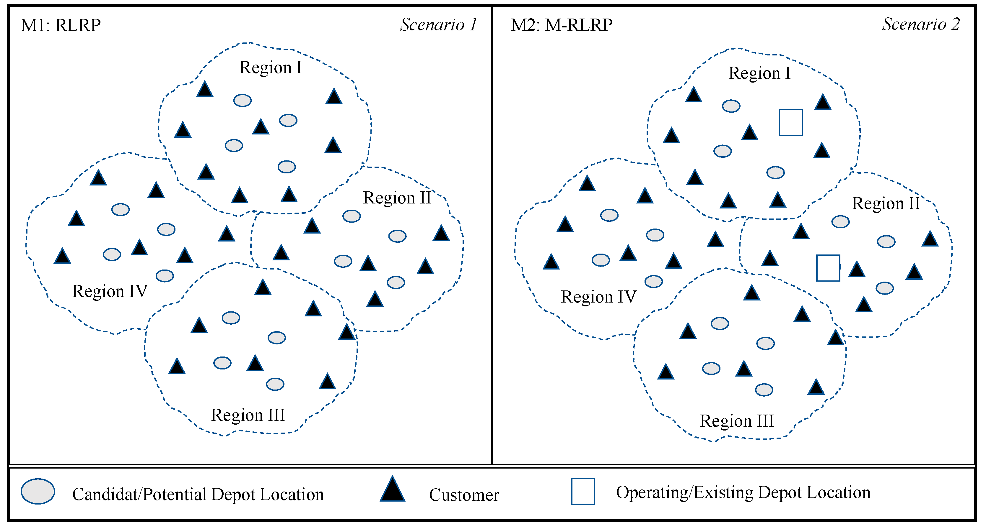
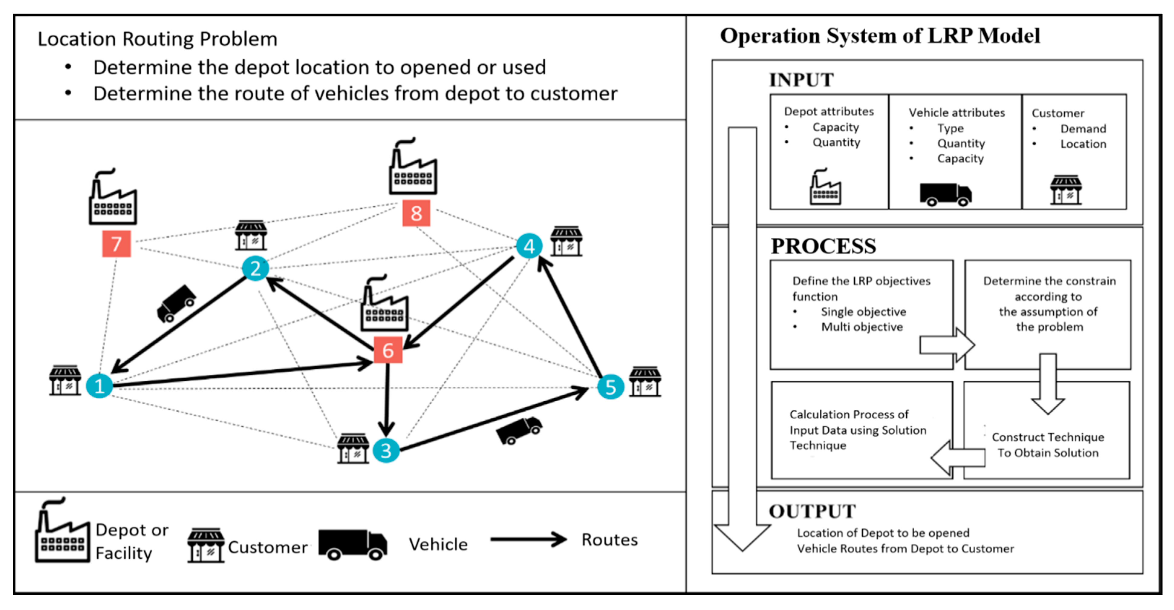
3.1. Regional Location Routing Problem

We take research conducted by Prins et al. [35] for the capacitated location routing problem as a reference model to develop the RLRP model. The formal mathematical model for the capacitated location problem is presented as follows. Let G represent a graph G = ( V , E ) , with G resembling a network containing V , a non-empty set containing vertices. In this case, V represents a set of nodes consisting of a subset l of m potential depot sites and a subset J = V | I from n customers. Here, E is a set of edges connecting each pair of nodes in V . Each edge ( i , j ) E is associated with travel costs c i j . Each depot i I has a capacity ( W i ) and has a depot opening cost ( O i ). Each customer has demand d j and must be fulfilled by a single vehicle. A number K of identical vehicles with capacity Q is available. Each vehicle starting the route and coming from depot i has fixed costs F i associated with the depot. Every vehicle route must start and end at the same depot. The total load carried by the vehicle must not exceed the capacity of the vehicle.
By considering the minimum number of depots in each area or region, this study denotes h to represent a particular region, while I h represents the depot set located in region h . The minimum number of depots to be available in each region is denoted by w . The model’s objective is to determine which depots should be opened in each region and the route for each vehicle from the depot to the customer to minimize the total cost.
We define binary variables y i = 1 if depot i is opened, f i j = 1 if customer j is assigned to depot i , and x j l k = 1 if edge ( j , l ) is traversed from j to l in the route performed by the vehicle k K . The problem formulation for RLRP goes as follows.
Minimize
Z = i I O i y i + i V j V k K c i j x i j k + k K i I j J F i x i j k
Subject to:
k K i V x i j k = 1 ,   j J
j J i V d j x i j k Q ,   k K
j J d j f i j W i y i ,   i I
j V x i j k j V x j i k = 0 ,   i V ,   k K
i I j J x i j k 1 ,   k K
i S j J x i j k | S | 1 ,   S J
u J x i u k + u V \ { j } x u j k 1 + f i j ,   i I ,   j J ,   k K
i I h y i w ,   h = 1 , , r
x i j k { 0 , 1 } ,   i I ,   j J ,   k K
y i { 0 , 1 } ,   i I
f i j { 0 , 1 } ,   i I ,   j V
The objective function (1) is the sum of depot opening costs and the routing costs, including the travel costs and the fixed costs associated with vehicle usages. Constraint (2) ensures that each customer belongs to one route and has only one predecessor in the route. Constraints (3) and (4) are capacity constraints associated with routes and depots, respectively. Constraints (5) and (6) guarantee the continuity of each route so that each route terminates at the depot where the route starts. Constraint (7) is a sub-tour elimination constraint. Constraint (8) ensures that a customer must be assigned to a depot if a route connects to the customer. Constraint (9) ensures that the minimum number of depots are available in every region. Finally, constraints (10)–(12) are for the binary variable.

3.2. Multi-Depot Regional Location Routing Problem
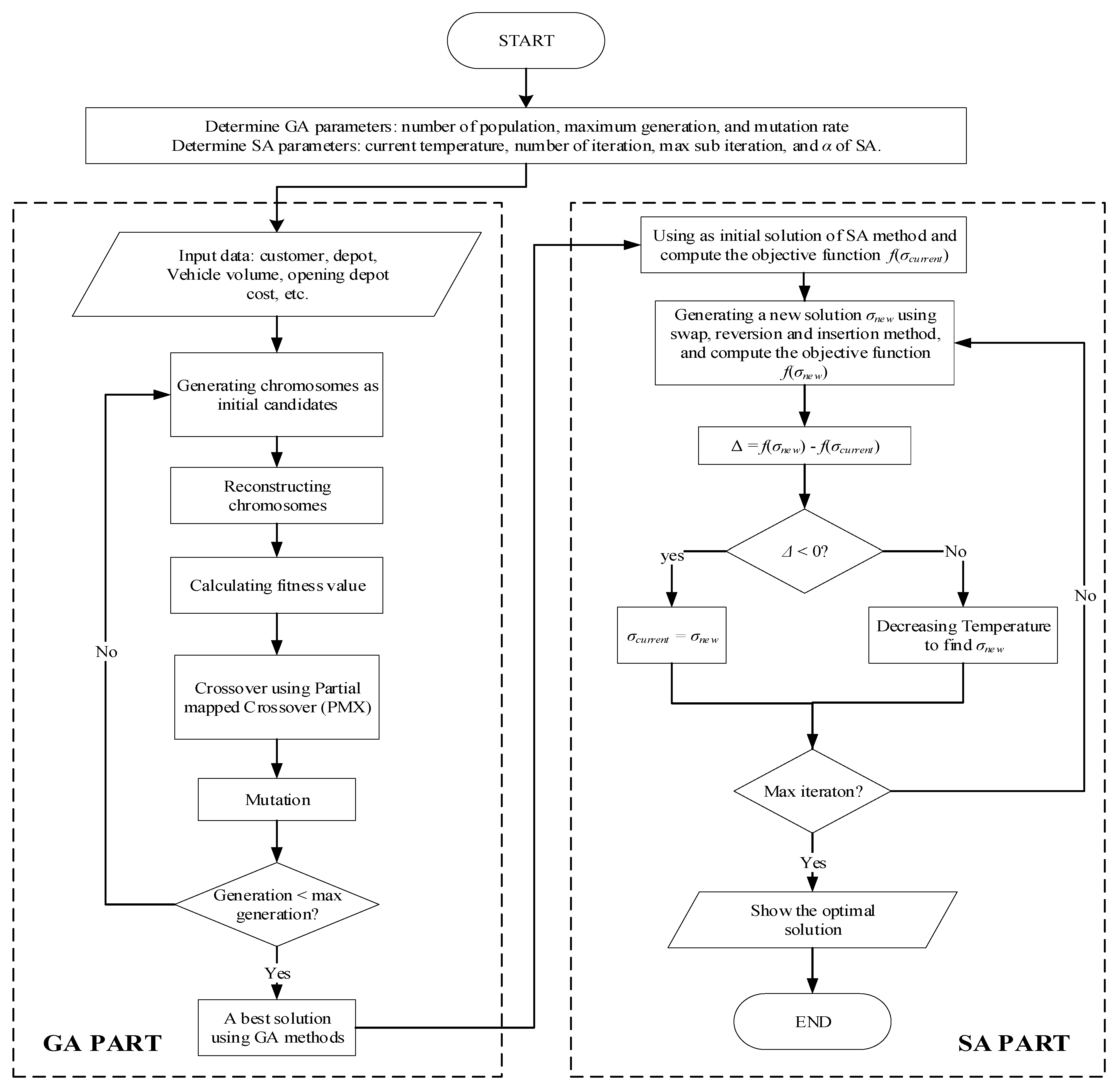
The multi-depot regional location routing problem (MRLRP) is a variant of the regional location routing problem (RLRP). MRLRP was developed to answer the need for deciding which depot should be opened and closed, including the route of vehicles originating from each depot. The decision of MRLRP is more complex than RLRP because it also determines which depots should be opened and closed in each region. In the MRLRP model, the depots are categorized into present depots and candidate depots. The present depots are depots that are currently operating or in use, denoted by I p . The candidate depots are unused depots that can be chosen as a new depot, denoted by I c . Therefore, the set of depots I consists of I p and I c , I = I p I c . Since we consider two types of depots, we introduce L i as the fixed cost of having depot i in the solution. If depot i is a depot that is not already present or a depot candidate, then L i will have a relatively large positive value; otherwise, it will denote the cost (gain) of the closing depot i and will possibly have a negative value. The objective function for MRLRP goes as follows.
Minimize
Z = i I O i y i + i V j V k K c i j x i j k + k K i I j J F i x i j k + i I c L i y i + i I p L i ( 1 y i )
The objective function (13) minimizes the sum of fixed-opening depot costs and routing costs, including the travel costs and the fixed costs associated with vehicle usages. Several decision variables are binary that can be taken, for example, variable y i = 1 if depot i is opened, with i I p (for present depot) or i I c (for candidate depot). Here, x j l k = 1 if edge ( j , l ) is traversed from j to l in the route performed by the vehicle k K . Similar to RLRP, each depot i I has a specific capacity ( W i ) and has a depot opening cost ( O i ). Each vehicle starting the route and coming from depot i has fixed costs F i associated with the depot. The term c i j represents travel costs from i to j . Since MRLRP is a variant of RLRP, the constraints for MRLRP are the same as RLRP.

4. Solution Method

This section explains the solution method to solve the problem. Since RLRP and MRLRP are particular cases of LRP and LRP is an NP-hard problem, we consider using metaheuristics to solve the model. Although existing studies have made significant progress in developing solution approaches, it turns out that there are still fewer studies that implement GA in combination with SA to solve LRP. We propose a hybrid approach of GA and SA for two reasons: (1) GA may fail to converge to a global optimum since it explores too many search spaces, whereas (2) we could increase the solution quality using GA output as the initial solution for SA. Moreover, we adopt this approach because it is one of the more promising alternatives to deal with this class of problems and has proven to provide a good result for various types of routing-like problems [31,36,37]. The illustration of the hybrid method is shown in Figure 2.

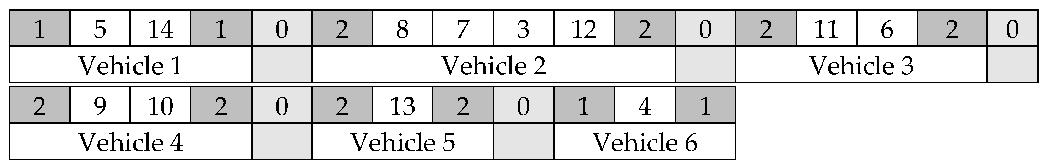
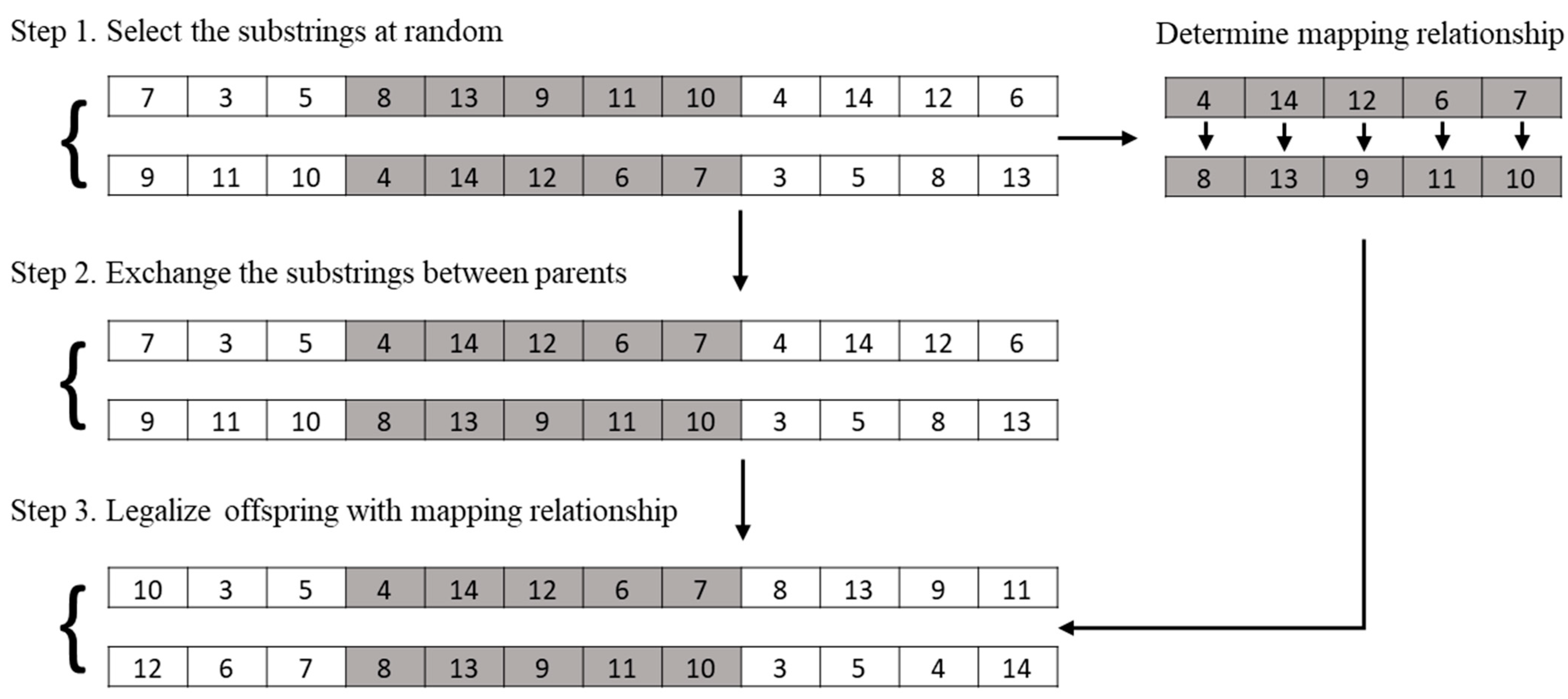
4.1. Genetic Algorithm

Before going into the technical details of our hybrid approach, we briefly explain the basic concept of GA. GA is a population-based metaheuristic that adopts the mechanism of genetic rules for the individual. Those individuals are following genetic rules to raise new offspring. GA starts with a population of solutions, and then it finds a better solution by applying genetic operators (selection, mutation, and crossover) over the individuals of each iteration. The critical issue when designing GA is to define the genetic operators carefully [18].
The first step that we need to prepare is all the information required in the model (customer attributes, depot attributes, vehicle attributes, and distance for each location) and the parameter for GA. The next step is generating chromosomes as initial candidates. In our approach, a solution is represented by a string of numbers consisting of a permutation of m depots denoted by the set { 1 , 2 , 3 , , m } , n potential customers denoted by the set { m + 1 , m + 2 , , m + n } , and N d u m m y zeros used to separate routes, in addition to the vehicle and depot capacity constraints. Suppose we have two candidate depots and twelve customers, as shown in Table 2. The vehicle capacity is 60, with the vehicle cost associated with depot ( F i ) equal to 10. The opening cost for each depot ( O i ) is equal to 1000. The distance for each node is calculated using the distance matrix API developed by Google based on latitude and longitude of each node. The asymmetric distance matrix is generated.
Based on Table 2, we generate chromosomes as initial candidates with a chromosome length equal to 14 (2 depot and 12 customers). Suppose we use 10 mutations for each iteration and generate the initial route, as shown in Appendix B.
For each chromosome, we insert a depot to serve the customer based on the maximum waste picked up by the vehicle. To determine which depot to serve the customer, we implement the shortest distance allocation method. We use dummy zero in the solution representation to separate the route for each vehicle. For example, in chromosome-1 on Appendix B, customers 5 and 14 will be served by depot 1 instead of 2 because depot 1 is the shortest distance from the node. By doing so, we are able to minimize the total distance for each route. The solution representation for chromosome-1 is shown in Figure 3.
Based on Figure 3, we use two depots and six vehicles to serve all the customers. The total cost (fitness value) for chromosome-1 is 123,117. By doing the same thing, we are able to calculate the fitness value for all chromosomes. The results are shown in Appendix C.
The next step is the selection process. The proposed method implements tournament selection for choosing the fittest candidates from the current generation in GA. These selected candidates are then passed on to the next generation. After selecting the individuals using tournament selection, we create a new generation by combining parent solutions to produce a new solution in GA. We apply partially matched crossover (PMX) to generate new offspring. PMX is the most frequently used crossover operator that Goldberg and Lingle proposed for the traveling salesman problem (TSP) [38]. The illustration of PMX in the proposed GA is shown in Figure 4.
Based on Figure 4, PMX starts by choosing parents from the previous selecting process. In this example, we choose chromosome-7 as parent-1, which has the lowest fitness value. Parent-2 is generated from parent-1 by shifting the order in parent-1. Step-1 chooses a random segment (substrings) and copies it from parent to child. It determines the mapping relationship between two substrings as references to select the position of the node. Step-2 exchanges the substrings between parents and checks whether any node is duplicated in the strings. Since we have the references from the mapping, we replace the duplicated node with another node following the mapping relationship. The rest of the offspring can be filled similarly with the parents.
The next step after crossover is conducting a mutation operator. The mutation operator is conducted to increase the probability of avoiding local solutions in GA. The mutation operator alters one or multiple genes in the children’s solutions after the crossover phase. Until the end criterion, GA improves the population using the operators mentioned above. Finally, the output of GA is used as the initial solution of the simulated algorithm.

4.2. Simulated Annealing

Simulated annealing (SA) is performed after an initial solution is created. In the beginning, we determine SA parameters, such as the current temperature, maximum outer iteration, maximum inner iteration, and cooling temperature coefficient. The proposed SA conducts two types of iterations: inner and outer.
Inner iteration focuses on finding the new solution based on the current solution utilizing the neighborhood moves. For inner iteration, we determine the maximum number of inner iterations to terminate the looping process. In contrast, outer iteration is used to control the temperature of SA. Two types of solutions are kept during the iterations of SA: σ c u r r e n t , which represents the current solution, and σ b e s t to represent the best-found solution. Initially, σ c u r r e n t is obtained from the initial solution, which is from the GA output. We implement roulette-wheel selection to create a neighborhood with the probability of 0.2, 0.5, and 0.3 for swap, reversion, and insertion, respectively. A new solution σ n e w is generated from one of three neighborhood moves.
After σ c u r r e n t is generated, the objective value of σ c u r r e n t is calculated. Let f ( σ ) represent the objective value of a solution σ . To determine whether σ c u r r e n t is accepted as σ n e w , a comparison between f ( σ c u r r e n t ) and f ( σ n e w ) is necessary. Consequently, Δ is defined as f ( σ n e w ) f ( σ c u r r e n t ) . If Δ < 0 , then σ n e w will replace σ c u r r e n t . However, if Δ > 0 , then σ n e w is not directly rejected and a random value r 1 ranging from 0 to 1 is generated. The neighborhood solution is accepted with the probability e ( Δ T ) . If r 1 < e ( Δ T ) , then σ n e w is accepted as σ c u r r e n t ; otherwise, σ n e w is rejected. This process continues until inner and outer iterations are completed. T is reduced by multiplying with a constant α .

5. Experimental Results and Discussion

This study develops two scenarios to provide an alternative solution for waste collection. Therefore, we implemented the model into the real problem adopted from the waste collection process in Bandung City, Indonesia. Before explaining the computational results of the proposed method, we briefly explain the situation and problem in the case study.

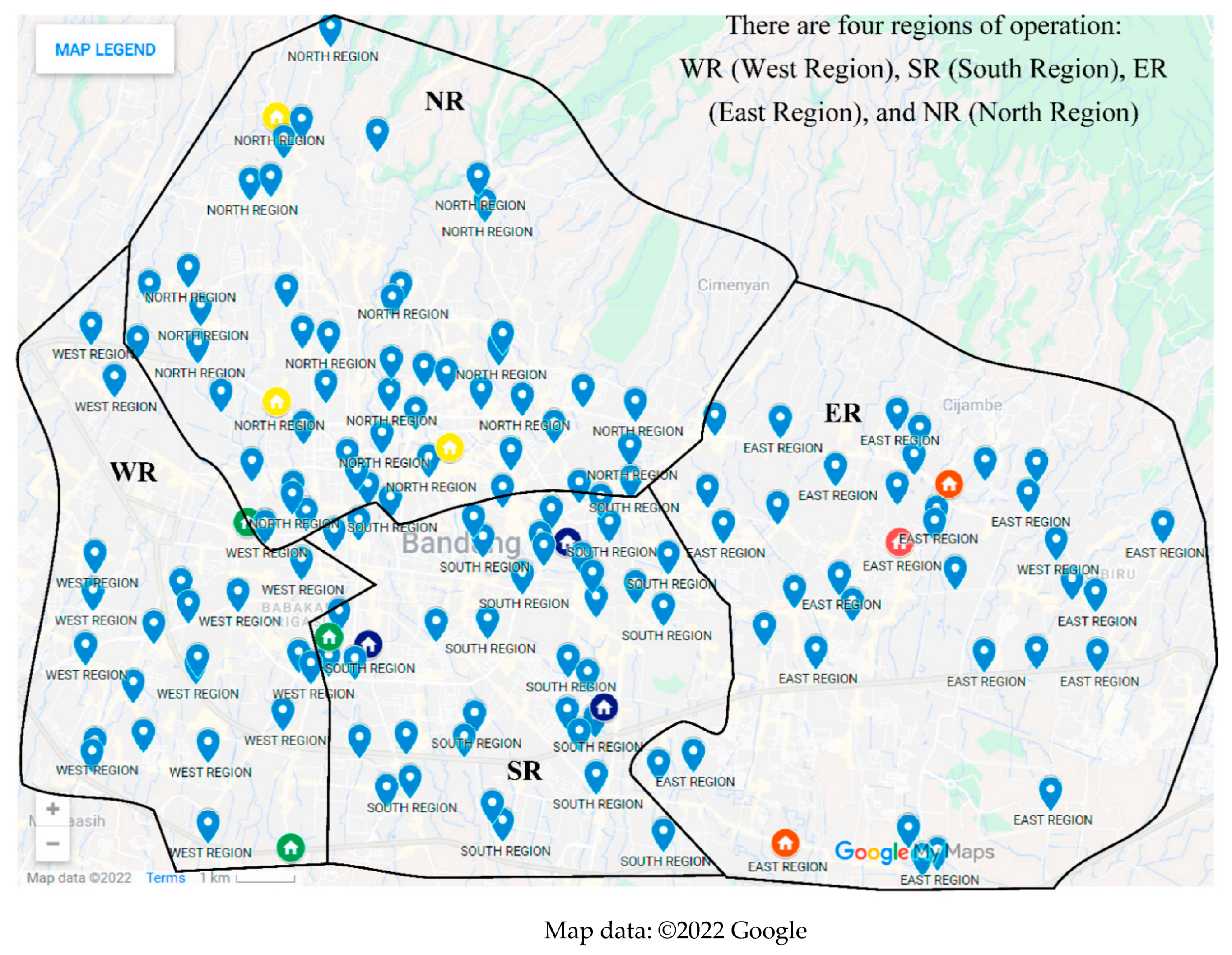
5.1. Case Study: Bandung

The increasing number of Bandung’s population has resulted in a greater volume of municipal waste. The volume of waste in Bandung in 2020 was 1735.99 M3/day, with the total population at 2,444,160 people, which continues to grow year by year [39]. To manage the waste in Bandung City, the local government selected PD Kebersihan to manage the waste problem. PD Kebersihan has conducted various innovations, such as a waste bank, composting, biodigester, bioconversion with maggots, and so forth; the waste disposed at the waste final processing site did drop. The final disposal location is the Sarimukti landfill (TPA) located in Sarimukti Village, Cipatat Subdistrict West Bandung Regency, which covers 25 Ha. The distance from Bandung City to the TPA location is 45 km. Therefore, it takes 1 to 2 h to travel to TPA. The Sarimukti landfill’s waste comes from Bandung City, Cimahi City, and West Bandung Regency.
Due to the large volume of waste and fuel and oil for transportation, a substantial cost is needed for this situation. Therefore, PD Kebersihan initiated a policy to increase the revenue from the billing sector by increasing the tariffs for waste services to overcome the high cost. PD Kebersihan also considered the application of new technology and setting the location of the depot. However, the problem is still a major challenge. The waste management system in Bandung is still centralized and only uses one central depot as a final waste collection for all four districts in Bandung. It causes the garbage collection systems to take a long time and incur high transportation costs. During the pandemic and LSR policy, PD Kebersihan faced more challenges collecting the waste for the four districts. Therefore, this research was conducted by developing two scenarios to deal with the waste problem in Bandung and, more specifically, to help PD Kebersihan.
To deal with the problem and implement the scenario, we collected the data from PD Kebersihan for the year 2016, including the waste disposal point, waste volume for each site, alternative location for final dumping point, vehicle capacity, and the costs associated with it. All the information that we used in the model can be downloaded at https://cutt.ly/1n660Md (accessed on 18 April 2022) An illustration of the Bandung City map and waste collection point is shown in Appendix D.
Based on the data provided by PD Kebersihan, we calculated the matrix of origins and destinations using the distance matrix API developed by Google for each node and obtained an asymmetric matrix distance. In total, there are 154 locations for temporary waste dumps in Bandung City. From these 154 locations, we generated 20 instances with various data sizes for each scenario. Both the RLRP and MRLRP have 20 data samples each, so the total number of instances we generated is 40. For each instance, we included the number of regions, the number of potential depots, the number of customers, the minimum number of depots for each region, the capacity of a vehicle, and cost components.
To generate the instances, we first determined and varied the number of location points, starting from the small size of 12 locations to the largest size of 154 locations. Next, we determined which regions will be sampled and the minimum number of depots opened. Location points were selected as candidate depots and other points in the same region as consumers to fulfil their requests according to the data taken from PD Kebersihan. It was ensured that the depot capacity could accommodate the consumer demand in the region to produce feasible solutions. The capacity of the vehicle was determined to be able to meet the demands of all the consumers. This study assumed that the number of vehicles is infinity to satisfy all the demands. Subsequent development can refer to previous instances by adding location points and varying the minimum number of depots required. The cost components attached to each component were assumed to be fixed and not dynamic. For the MRLRP case, we developed the instances from RLRP datasets by selecting one of the depots as the present depot and the other depots as candidate depots.

5.2. Experimental Results
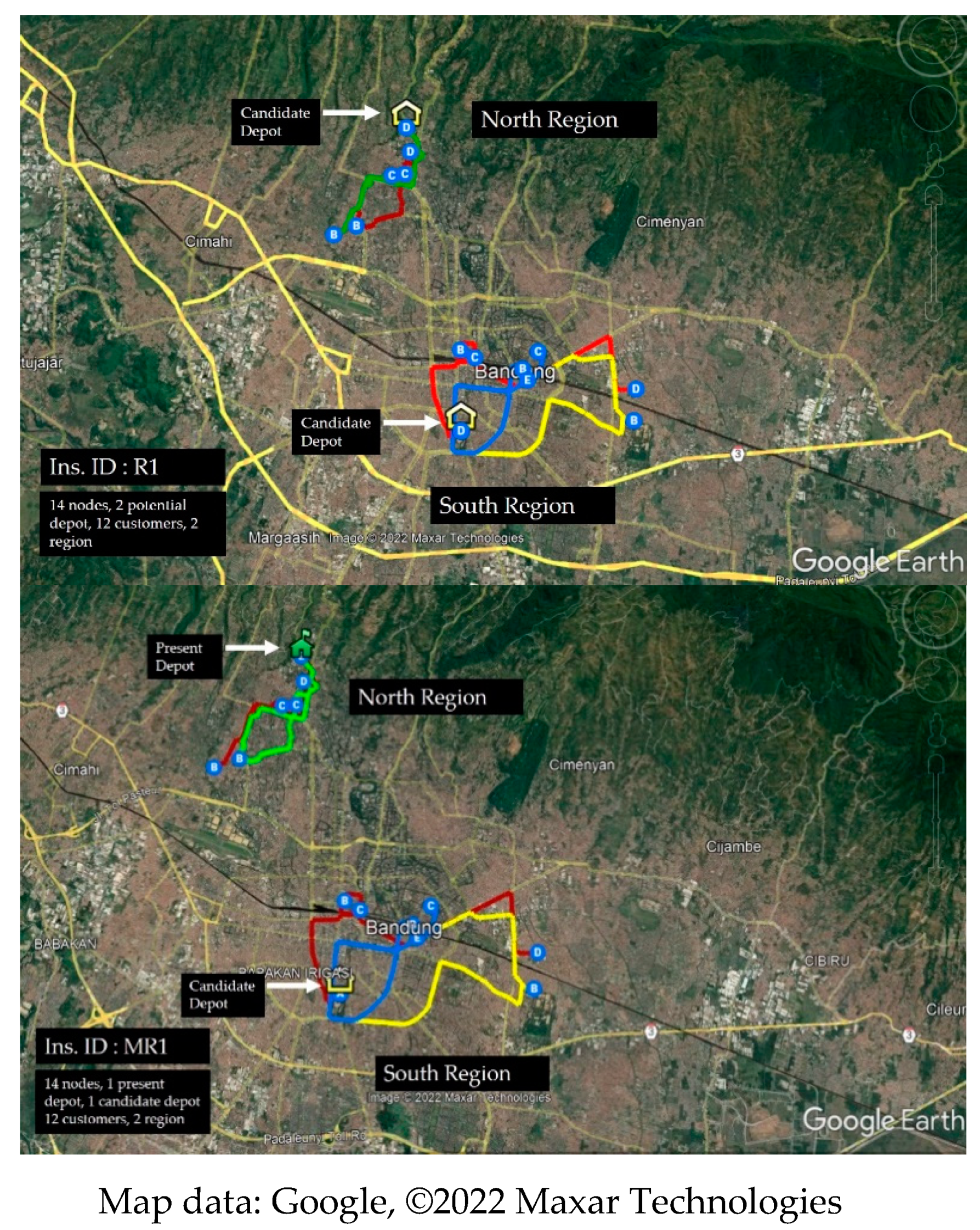
The proposed algorithm was implemented in Matlab. The experiments were conducted on a computer with an Intel Core i5-6400 CPU @ 2.70 Ghz. The mathematical model for the RLRP and MRLPR was solved using a Gurobi solver on the same machine.

5.2.1. RLRP Dataset

The proposed algorithm was tested on the RLRP dataset. The results appear in Table 3. We compared the results obtained by our developed GASA with the solution from the Gurobi solver. In Table 3, the BKS column represents the best solution provided by Gurobi, GA, and GASA. The following formula defines the performances of GA and GASA:
G a p a ( % ) = G A . O b j . ( best ) B K S B K S × 100 %
G a p b ( % ) = G A S A . O b j . ( best ) B K S B K S × 100 %
G a p c ( % ) = G A . O b j . ( best ) G A . O b j . ( a v g ) G A . O b j . ( a v g ) × 100 %
G a p d ( % ) = G A S A . O b j . ( best ) G A S A . O b j . ( a v g ) G A S A . O b j . ( a v g ) × 100 %
Based on Table 3, the smallest gap between GA and BKS is obtained for solving R1 and R2—i.e., 0.00%—while the largest gap reaches 0.91% from solving R19. GA performs better than Gurobi for solving the R14 dataset. The average gap of the objective result between GA and BKS is 0.38%. The proposed GASA outperforms Gurobi in quality solutions for solving R4, R7, R8, R10, and R14. The largest gap compared with BKS is obtained for solving R15, i.e., 0.11%. The average gap of objective results is 0.01%. GASA provides a better solution than GA in terms of solution quality because the input of GASA is developed from GA. However, for computational time, GA is faster, at an average of 40.83 s compared to GASA. Both GA and GASA, on average, have lower computational times than Gurobi.
Gurobi outperforms GASA, with the largest gap of 0.11% for solving R15. However, among 20 instances, Gurobi only solves 14 instances, with an average computational time of 12,342.69. Moreover, the optimal solution is obtained in solving five instances. In other instances, we set a maximum of 5 h to develop a feasible solution for Gurobi. With this setting, the Gurobi solver is expected to provide feasible outputs even though it does not reach the global optimum. Based on Table 3, we conclude that the proposed GASA is competitive in solving RLRP instances compared to Gurobi. In terms of computation time, GASA is, on average, faster than Gurobi.
Furthermore, we investigated the gap between the best solution and the average solution obtained by GA and GASA on each RLRP instance. The average gaps are −4.74% and −0.50% for GA and GASA, respectively. Based on the result, the gap value is relatively constant in each instance, and we conclude that the proposed algorithm is robust enough to solve RLRP.

5.2.2. MRLRP Dataset

The proposed algorithm is also tested on the MRLRP dataset. For the fundamental difference between the RLRP dataset and MRLRP dataset, in MRLRP, we consider two types of depots: present depot and candidate depot. As shown in Table 4, we conduct parameters for the two depot types. The results are summarized in Table 4. We compare the results obtained by our proposed GASA with BKS and calculate the gap following Formulas (14)–(17), as mentioned in the previous section.
Based on Table 4, the largest gap between GA and BKS is 1.78%, obtained for solving MR20. The average gap of GA for solving MRLRP instances is 0.64%. Although, for some instances, Gurobi outperforms GA, GA is able to solve all 20 instances, while Gurobi is only able to solve 14 of 20 instances. The largest gap between the proposed GASA and BKS is 0.07%, obtained for solving MR15. Both GA and GASA, on average, have lower computational time than Gurobi.
We further note that Gurobi outperforms GASA for solving MR3, MR11, MR15, and MR16. However, Gurobi can only solve 14 of 20 instances, with an average computational time of 10,870.15. Therefore, we conclude that our proposed algorithm is competitive versus the Gurobi solver.
We investigated the gap between the best solution and the average solution for GA and GASA for each instance to evaluate the robustness of the proposed algorithms. The average gap is −0.99% and −0.50 for GA and GAS, respectively. Therefore, we could conclude that, based on the experiment, the proposed algorithm is relatively robust to solve MRLRP.

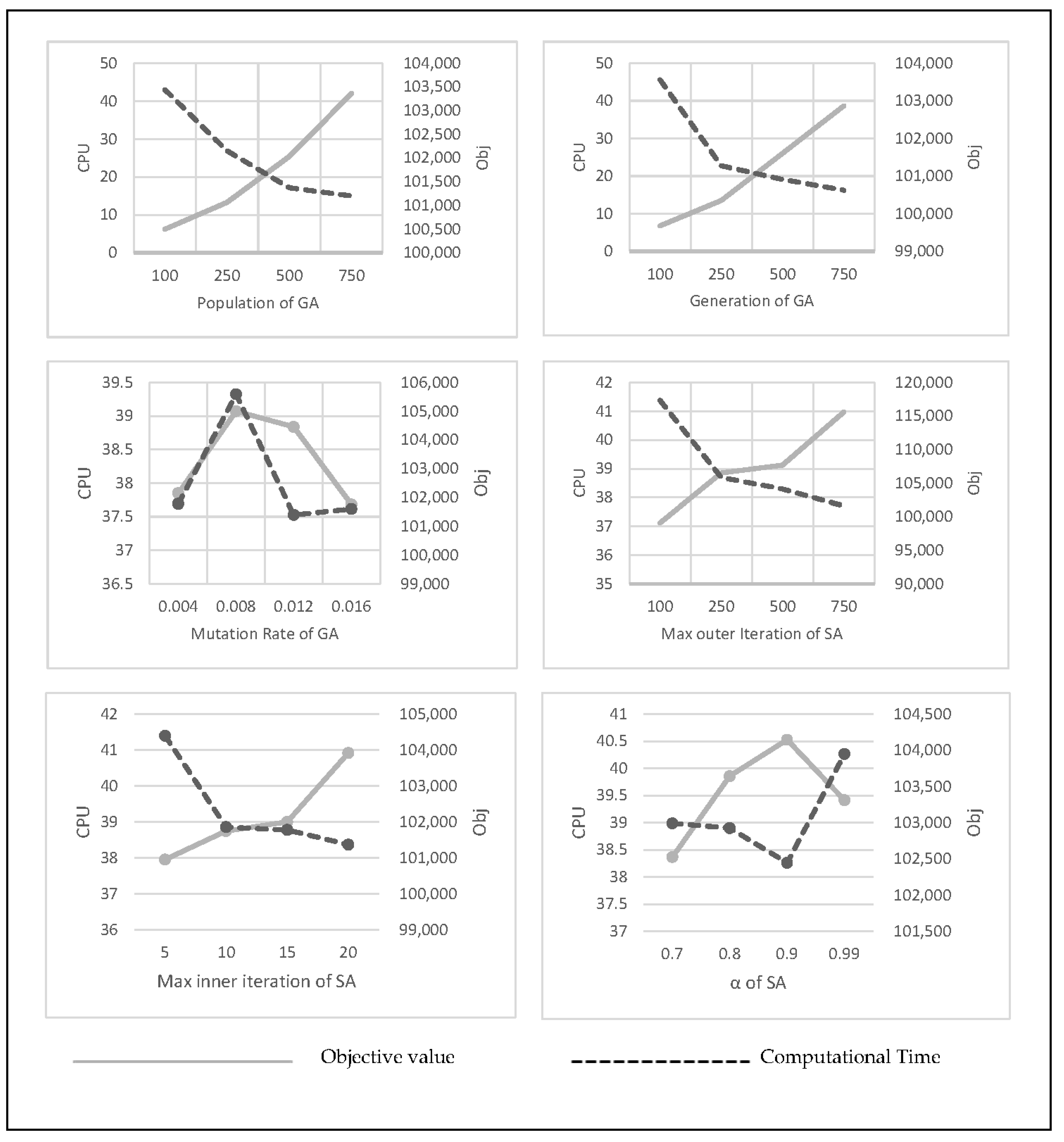
5.3. Sensitivity Analysis for GA and SA Parameters

The sensitivity analysis aims to investigate the relationships among GA, SA, and solution output. We examine the effect of parameter configuration for each algorithm on the CPU time and objective value. This study conducts one-at-a-time (OAT) sensitivity measures to analyze the effects of parameters on the output. Using OAT, we repeatedly vary one parameter at a time while holding the others fixed. In this study, we use four value levels for each parameter to determine the proper configuration of the proposed algorithm. Appendix E represents the output of our proposed algorithm for different parameter values.
Based on Appendix E, we present each parameter’s effect on the objective value and computational time in Figure 5. We see that higher levels of population and generation parameter for GA increase the computational time but do increase the quality of the solution (case of minimization). However, for the mutation rate of GA, the experimental study shows that the mutation rate’s size does not directly affect the quality of the results and computational time. Therefore, in this study, for GA, we implement the size of population = 750, number of generations = 750, and mutation rate = 0.012.
The parameters of SA that we measure in this study are the maximum number of outer iterations, the maximum number of inner iterations, and the value of α. We show that, the higher the number of iterations (outer or inner) is, the better the quality of the solution will be, but the computation time will also increase. For the level of α, based on the experiment, an increase in the α value is not directly proportional to the quality of the solution and the computational time. Therefore, in this study, for SA, we set the maximum number of outer iterations = 750, the maximum number of inner iterations = 20, and α = 0.9.

5.4. Discussion

We define two sets of municipal waste management scenarios and indicate them as scenarios S1 and S2. In scenarios S1 and S2, we assume a minimum number of depots for each region. Although our proposed scenarios meet the criteria when the LSR policy is implemented, we also analyze that these two scenarios can provide benefits even though the LSR policy is no longer implemented. Insofar as the status quo only uses one final depot/landfill to handle all the waste in the city, the consequences of this policy are (1) a large area for waste is needed, (2) a long time to transport the waste due to the distance is required, and (3) a high environmental impact occurs due to the waste volume at the landfill. With the scenarios that we develop, some of the impacts are (1) reducing the need for large areas because the waste collection is carried out in each region, (2) the waste collection is faster because the distance to the depot is closer than before, and (3) the faster the waste is processed, the more it will reduce its environmental impact. However, for implementing the model, we realize that additional costs are needed to facilitate equipment at the new depot because, previously, the depot point was only for collecting waste, not processing waste. The cost depends on the location, so our model has not covered it in detail. Another critical note at the time of implementation was the need for information on the social and environmental impact analysis in advance to open the depot so the decision-maker can calculate the necessary steps.
This paper proposes two scenarios represented by mathematical programming models: RLRP and MRLRP. Besides these two, the mathematical model can also solve the capacitated location routing problem (CLRP) since it is developed from the CLRP. However, to implement the RLRP and MRLRP into the CLRP, we need to adjust the constraints and parameters. Since the CLRP does not consider the minimum number of depots for each region, if we only consider one region and the minimum number of depots equals zero, then the RLRP will become a problem of the CLRP. This situation also applies to the MRLRP model; if we assume that there is no present depot, it will also become the problem of CLRP.
Based on the experiments, we compare the output of the mathematical model through commercial solver Gurobi and a metaheuristic. As shown in Table 3 and Table 4, the commercial solver cannot solve all the instances because of the complexity of the model. Although we already limit the computational time to 5 h, the commercial solver can only solve 28 of 40 instances. The limitation of the commercial solver leads to the development of a heuristic, i.e., genetic algorithm and simulated annealing. However, using the result obtained from the commercial solver allows us to evaluate the performance of the proposed algorithm.
The proposed GASA provides a competitive solution compared with Gurobi to solve the RLRP and MRLRP. However, for other LRP problems, we suggest conducting further experiments since each algorithm has its limitations. The disadvantages of metaheuristics are a weak local search and the role of randomness. We run several experiments to determine the most appropriate parameter for the proposed algorithms to handle these weaknesses. We run at least 20 times for each algorithm to obtain the best solution on each instance.
The critical factors of GA in providing a good solution for the RLRP and MRLRP are the GA operator and the parameter tuning. Therefore, utilizing the parameter value based on the experiments, we explore the wide range of solution spaces to find a promising solution. For SA, the critical factors are utilizing neighborhood moves, the acceptance criteria, and tuning parameters. Neighborhood moves increase the search space of finding the solution, the acceptance criterion escapes from local optima, and the tuning parameters achieve a good performance. There are two important issues in search strategies: exploring the search space and exploiting the best solution. Although GA and SA include mechanisms to manipulate the explore (diversification) and exploit (intensification) aspects of the search space, we found that, in our case, GA performs better in exploring the search space. This is due to the crossover operator tending to perform a widespread search. In contrast, SA can take an unchanged or effective solution as a new current solution with an exact probability so that the algorithm can tune itself in a near-optimal solution. Therefore, the two algorithms can complement each other to produce a better solution.
In terms of complexity and computational time, the complexity of the proposed GASA is located in (1) the objective calculation procedure and (2) the exploration procedure to find a new solution. The other remaining parts can be obtained in a constant time.
The procedures of objective calculation have complexity O ( | n + m | ) because they sequentially evaluate all nodes (i.e., n customers and m depots) in the solution representation. Consequently, the increasing number of nodes raises the time to generate a solution. The exploration procedures include the genetic operators and SA neighborhood moves. The genetic operators consist of selection, mutation, and crossover. The selection requires a constant time, while the other two depend on the locations of the selected nodes. For the mutation, the complexity is O ( n t ) , where n t represents the number of nodes that need to be mutated. For the crossover, we implement PMX, and the complexity is O ( 2 n x ) , where n x represents the number of nodes on the substrings that we choose as the mapping references. The SA neighborhood moves consist of swap, insertion, and inversion. The swap requires a constant time, while the other two depend on the locations of the selected nodes. For insertion, the complexity is O ( n i ) , where n i represents the number of nodes that need to be shifted due to the insertion move. For the inversion, the complexity is O ( n v / 2 ) , where n v is the number of nodes located between the selected two nodes (including the two nodes) in the inversion move. Based on the complexities mentioned above, they become the main reason that the sizes of the dataset influence the computational time of GASA.
We also conduct statistical tests to evaluate the performance of our proposed algorithm and implement the Wilcoxon signed-rank test to measure the significance of our proposed method compared with BKS and Gurobi. To analyze and test the hypothesis, we apply the confidence level of alpha equal to 0.004. Therefore, if the p-value is less than the alpha, we conclude that the methods are different. Based on Appendix F, in terms of solution value, for GA to solve the RLRP, the p-value is less than 0.05, which means that there is a significant difference between GA with Gurobi and GA with BKS. On the other hand, the p-value results of GASA and Gurobi are more than 0.05, denoting that the result is not significantly different, so GASA provides a competitive result compared with Gurobi for the RLRP dataset. However, in terms of running time, both GA and GASA have a p-value less than the alpha, and, hence, the running time is significantly different from Gurobi. We conclude that, statistically, GASA can provide competitive results at a faster running time compared with Gurobi. For the MRLRP datasets, GA obtains a p-value of less than 0.05, indicating that there is a significant difference in the GA results compared with Gurobi and BKS. On the other side, the GASA result for the solution test has a p-value more than the alpha, meaning that there is no significant difference for GASA to obtain a solution for the MRLRP, and thus the proposed algorithm is competitive.

6. Conclusions

This research proposes a new variant of the LRP, named RLRP and MRLRP, by considering the minimum number of depots for each region and two types of depots and proposes two mathematical models and a hybrid algorithm. Moreover, we generate a new set of instances from the real example adopted from PD Kebersihan in Bandung City to provide a more realistic illustration of the waste problem since the problem has never been dealt with in previous works (see sample illustration of the result in Appendix G).
We further analyze the performance of the proposed algorithm in solving both RLRP and MRLPR instances. For the RLRP dataset, GASA obtains near-optimal results, with the highest gap of 0.11% compared to BKS. For the MRLRP dataset, GASA has the highest gap of 0.07% versus BKS. The results indicate that the proposed method provides competitive results and a reasonable computational time compared to the commercial solver.
Several future directions that could be considered are noted as follows. Since this is a new problem, future works may improve the solutions. In this study, we consider homogeneous vehicles. Therefore, a follow-up study could consider a heterogeneous vehicle. Moreover, a multi-objective experiment could be conducted to minimize the cost and maximize the service level. Another interesting aspect of research could be conducted by comparing the performance of the proposed algorithm to solve a different problem or benchmark instances in the LRP. The development of better solution methods can also be conducted in further research, such as embedding SA into GA, particle swarm optimization (PSO), differential evolution (DE), ant colony optimization (ACO), and other metaheuristic algorithms. Lastly, future research can develop different scenarios to solve the waste problems.

Author Contributions

Conceptualization, V.F.Y. and H.S.; methodology, V.F.Y., G.A., H.S. and S.-W.L.; software, G.A., H.S., M.K.E. and S.-W.L.; validation, V.F.Y., G.A., H.S. and M.K.E.; formal analysis, G.A. and H.S.; investigation, H.S.; resources, V.F.Y., S.-W.L. and M.K.E.; data curation, G.A. and H.S.; writing—original draft preparation, V.F.Y., G.A. and H.S.; writing—review and editing, V.F.Y., G.A., H.S., S.-W.L. and M.K.E.; visualization, H.S. and G.A.; supervision, V.F.Y. and S.-W.L.; project administration, V.F.Y.; funding acquisition, V.F.Y. and S.-W.L. All authors have read and agreed to the published version of the manuscript.

Funding

This research is partially supported by the Ministry of Science and Technology of the Republic of China (Taiwan) under grant MOST 106-2410-H-011-002-MY3 and the Center for Cyber-Physical System Innovation from The Featured Areas Research Center Program within the framework of the Higher Education Sprout Project by the Ministry of Education (MOE) in Taiwan. The work of S.-W. Lin is supported in part by the Ministry of Science and Technology, Taiwan under Grant MOST 109-2410-H-182-009MY3, and in part by the Linkou Chang Gung Memorial Hospital under Grant BMRPA19.

Institutional Review Board Statement

Not applicable.

Informed Consent Statement

Not applicable.

Data Availability Statement

Not applicable.

Acknowledgments

The authors are grateful to PD Kebersihan in Bandung City, and especially to the General Director, Gun Gun Saptari Hidayat, for the opportunity to conduct the research. The authors are particularly grateful to Hangga T. Saputra, the Head of Administration and Operational Division of PD Kebersihan, for the professional expertise and immense knowledge in waste management in Bandung and the interview process.

Conflicts of Interest

The authors declare no conflict of interest.

Appendix A

Figure A1. Operation system of the LRP model.
Mathematics 10 02131 g0a1

Appendix B

Table A1. Chromosome and permutation for each customer.
ChromosomeCustomer Node
151487312116910134
297111461031384125
310735141349128116
431051289117614413
571381012395641411
668149341312711105
773581391110414126
831412136548117910
910814121113456793
1048510133914116127

Appendix C

Table A2. Fitness value for each chromosome.
ChromosomeCustomer NodeFitness Value
151487312116910134123,117
297111461031384125129,960
310735141349128116109,699
431051289117614413112,264
571381012395641411101,833
668149341312711105132,268
77358139111041412684,500
831412136548117910112,148
91081412111345679396,237
1048510133914116127133,538
Bold value denotes the smallest value.

Appendix D

Figure A2. Bandung city map and waste collection locations.
Mathematics 10 02131 g0a2

Appendix E

Table A3. Tested parameter values for GA and SA.
Genetic AlgorithmSimulated Annealing
ParameterLevelObj.CPUParameterLevelObj.CPU
Population100103,4436.22Max outer iterations100117,35337.12
250102,15013.30 250105,83438.86
500101,37225.42 500104,12439.13
750101,19942.06 750101,60540.98
Generation100103,5596.79Max inner iterations5104,39437.96
250101,27613.52 10101,85938.75
500100,90926.05 15101,78139.01
750100,62438.67 20101,37240.92
Mutation rate0.004101,78137.85α0.7102,99138.37
0.008105,60039.08 0.8102,92639.86
0.012101,39938.84 0.9102,44740.53
0.016101,60437.68 0.99103,94839.41

Appendix F

Table A4. The results of the Wilcoxon signed-rank test on the solution value and running time for RLRP and MRLRP datasets.
GA vs.GASA vs.
BKSGurobiBKSGurobi
RLRP
datasets
Test on solution value
W−3.724−2.667−2.366−1.020
p-value0.0000.0180.0080.308
Test on running time
W −3.233 −3.233
p-value 0.001 0.001
MRLRP datasets Test on solution value
W−3.823−3.180−1.826−0.415
p-value0.0000.0010.0680.678
Test on running time
W −3.170 −3.107
p-value 0.002 0.002

Appendix G

Figure A3. The sample illustration for RLRP and MRLRP solutions on Google Earth.
Mathematics 10 02131 g0a3

References

  1. Boysen, N.; Fedtke, S.; Schwerdfeger, S. Last-mile delivery concepts: A survey from an operational research perspective. OR Spectr. 2020, 43, 1–58. [Google Scholar] [CrossRef]
  2. Haugland, D.; Ho, S.C.; Laporte, G. Designing delivery districts for the vehicle routing problem with stochastic demands. Eur. J. Oper. Res. 2007, 180, 997–1010. [Google Scholar] [CrossRef]
  3. Carlsson, J.G. Dividing a territory among several vehicles. INFORMS J. Comput. 2012, 24, 565–577. [Google Scholar] [CrossRef] [Green Version]
  4. Lei, H.; Laporte, G.; Liu, Y.; Zhang, T. Dynamic design of sales territories. Comput. Oper. Res. 2015, 56, 84–92. [Google Scholar] [CrossRef]
  5. Ouhader, H.; El Kyal, M. Combining facility location and routing decisions in sustainable urban freight distribution under horizontal collaboration: How can shippers be benefited? Math. Probl. Eng. 2017, 2017, 8687515. [Google Scholar] [CrossRef]
  6. Mara, S.T.W.; Kuo, R.; Asih, A.M.S. Location-routing problem: A classification of recent research. Int. Trans. Oper. Res. 2021, 28, 2941–2983. [Google Scholar] [CrossRef]
  7. Yu, V.F.; Lin, S.-W.; Lee, W.; Ting, C.-J. A simulated annealing heuristic for the capacitated location routing problem. Comput. Ind. Eng. 2010, 58, 288–299. [Google Scholar] [CrossRef]
  8. Dib, O.; Moalic, L.; Manier, M.A.; Caminada, A. An advanced GA–VNS combination for multicriteria route planning in public transit networks. Expert Syst. Appl. 2017, 72, 67–82. [Google Scholar] [CrossRef] [Green Version]
  9. Jacobsen, S.K.; Madsen, O.B. A comparative study of heuristics for a two-level routing-location problem. Eur. J. Oper. Res. 1980, 5, 378–387. [Google Scholar] [CrossRef]
  10. Yu, V.F.; Lin, S.-Y. A simulated annealing heuristic for the open location-routing problem. Comput. Oper. Res. 2015, 62, 184–196. [Google Scholar] [CrossRef]
  11. Zhang, X.; Tang, L. A new hybrid ant colony optimization algorithm for the vehicle routing problem. Pattern Recognit. Lett. 2009, 30, 848–855. [Google Scholar] [CrossRef]
  12. Fazayeli, S.; Eydi, A.; Kamalabadi, I.N. A model for distribution centers location-routing problem on a multimodal transportation network with a meta-heuristic solving approach. J. Ind. Eng. Int. 2018, 14, 327–342. [Google Scholar] [CrossRef] [Green Version]
  13. Rabbani, M.; Heidari, R.; Yazdanparast, R. A stochastic multi-period industrial hazardous waste location-routing problem: Integrating NSGA-II and Monte Carlo simulation. Eur. J. Oper. Res. 2019, 272, 945–961. [Google Scholar] [CrossRef]
  14. Peng, Z.; Manier, H.; Manier, M.-A. Particle swarm optimization for capacitated location-routing problem. IFAC-PapersOnLine 2017, 50, 14668–14673. [Google Scholar] [CrossRef]
  15. Panicker, V.V.; Reddy, M.V.; Sridharan, R. Development of an ant colony optimisation-based heuristic for a location-routing problem in a two-stage supply chain. Int. J. Value Chain. Manag. 2018, 9, 38–69. [Google Scholar] [CrossRef]
  16. Escobar, J.W.; Linfati, R.; Baldoquin, M.G.; Toth, P. A Granular Variable Tabu Neighborhood Search for the capacitated location-routing problem. Transp. Res. Part B Methodol. 2014, 67, 344–356. [Google Scholar] [CrossRef]
  17. Schneider, M.; Löffler, M. Large composite neighborhoods for the capacitated location-routing problem. Transp. Sci. 2019, 53, 301–318. [Google Scholar] [CrossRef]
  18. Derbel, H.; Jarboui, B.; Hanafi, S.; Chabchoub, H. Genetic algorithm with iterated local search for solving a location-routing problem. Expert Syst. Appl. 2012, 39, 2865–2871. [Google Scholar] [CrossRef]
  19. Karaoglan, I.; Altiparmak, F. A memetic algorithm for the capacitated location-routing problem with mixed backhauls. Comput. Oper. Res. 2015, 55, 200–216. [Google Scholar] [CrossRef]
  20. Khalili-Damghani, K.; Abtahi, A.-R.; Ghasemi, A. A new bi-objective location-routing problem for distribution of perishable products: Evolutionary computation approach. J. Math. Model. Algorithms Oper. Res. 2015, 14, 287–312. [Google Scholar] [CrossRef]
  21. Alinaghian, M.; Goli, A. Location, allocation and routing of temporary health centers in rural areas in crisis, solved by improved harmony search algorithm. Int. J. Comput. Intell. Syst. 2017, 10, 894–913. [Google Scholar] [CrossRef] [Green Version]
  22. Wang, Z.; Leng, L.; Wang, S.; Li, G.; Zhao, Y. A hyperheuristic approach for location-routing problem of cold chain logistics considering fuel consumption. Comput. Intell. Neurosci. 2020, 2020, 8395754. [Google Scholar] [CrossRef] [PubMed]
  23. Wu, X.; Nie, L.; Xu, M. Designing an integrated distribution system for catering services for high-speed railways: A three-echelon location routing model with tight time windows and time deadlines. Transp. Res. Part C Emerg. Technol. 2017, 74, 212–244. [Google Scholar] [CrossRef]
  24. Suksee, S.; Sindhuchao, S. GRASP with ALNS for solving the location routing problem of infectious waste collection in the Northeast of Thailand. Int. J. Ind. Eng. Comput. 2021, 12, 305–320. [Google Scholar] [CrossRef]
  25. Gogna, A.; Tayal, A. Metaheuristics: Review and application. J. Exp. Theor. Artif. Intell. 2013, 25, 503–526. [Google Scholar] [CrossRef]
  26. Beheshti, Z.; Shamsuddin, S.M.H. A review of population-based meta-heuristic algorithms. Int. J. Adv. Soft Comput. Appl 2013, 5, 1–35. [Google Scholar]
  27. Jaddi, N.S.; Abdullah, S. Global search in single-solution-based metaheuristics. Data Technol. Appl. 2020, 54, 275–296. [Google Scholar] [CrossRef]
  28. Samsuddin, S.; Othman, M.S.; Yusuf, L.M. A review of single and population-based metaheuristic algorithms solving multi depot vehicle routing problem. Int. J. Softw. Eng. Comput. Syst. 2019, 4, 80–93. [Google Scholar] [CrossRef]
  29. Jeon, G.; Leep, H.R.; Shim, J.Y. A vehicle routing problem solved by using a hybrid genetic algorithm. Comput. Ind. Eng. 2007, 53, 680–692. [Google Scholar] [CrossRef]
  30. Sitek, P.; Wikarek, J. Capacitated vehicle routing problem with pick-up and alternative delivery (CVRPPAD): Model and implementation using hybrid approach. Ann. Oper. Res. 2019, 273, 257–277. [Google Scholar] [CrossRef] [Green Version]
  31. Wang, C.-H.; Lu, J.-Z. A hybrid genetic algorithm that optimizes capacitated vehicle routing problems. Expert Syst. Appl. 2009, 36, 2921–2936. [Google Scholar] [CrossRef]
  32. Rodríguez-Martín, I.; Salazar-González, J.-J.; Yaman, H. A branch-and-cut algorithm for the hub location and routing problem. Comput. Oper. Res. 2014, 50, 161–174. [Google Scholar] [CrossRef] [Green Version]
  33. Ahmadi-Javid, A.; Amiri, E.; Meskar, M. A profit-maximization location-routing-pricing problem: A branch-and-price algorithm. Eur. J. Oper. Res. 2018, 271, 866–881. [Google Scholar] [CrossRef]
  34. Nadizadeh, A.; Nasab, H.H. Solving the dynamic capacitated location-routing problem with fuzzy demands by hybrid heuristic algorithm. Eur. J. Oper. Res. 2014, 238, 458–470. [Google Scholar] [CrossRef]
  35. Prins, C.; Prodhon, C.; Ruiz, A.; Soriano, P.; Wolfler Calvo, R. Solving the capacitated location-routing problem by a cooperative Lagrangean relaxation-granular tabu search heuristic. Transp. Sci. 2007, 41, 470–483. [Google Scholar] [CrossRef]
  36. Ho, W.; Ho, G.T.; Ji, P.; Lau, H.C. A hybrid genetic algorithm for the multi-depot vehicle routing problem. Eng. Appl. Artif. Intell. 2008, 21, 548–557. [Google Scholar] [CrossRef]
  37. Marinakis, Y.; Marinaki, M. A hybrid genetic–Particle Swarm Optimization Algorithm for the vehicle routing problem. Expert Syst. Appl. 2010, 37, 1446–1455. [Google Scholar] [CrossRef]
  38. Kora, P.; Yadlapalli, P. Crossover operators in genetic algorithms: A review. Int. J. Comput. Appl. 2017, 162, 34–36. [Google Scholar] [CrossRef]
  39. Badan Pusat Statistik Kota Bandung. Bandung Municipality in Figures 2021; Bandung, B.K., Ed.; BPS Kota Bandung: Bandung, Indonesia, 2021; Available online: https://bandungkota.bps.go.id/publication/2021/02/26/2fb944aeb2c1d3fe5978a741/kota-bandung-dalam-angka-2021.html (accessed on 18 April 2022).
Figure 1. Illustration of scenario 1 and scenario 2.
Mathematics 10 02131 g001
Figure 2. The hybrid mechanism for GASA.
Mathematics 10 02131 g002
Figure 3. Solution representation for chromosome-1.
Mathematics 10 02131 g003
Figure 4. An illustration of partially mapped crossover (PMX), the proposed GA.
Mathematics 10 02131 g004
Figure 5. Effect of GA and SA parameters on computational time and objective value.
Mathematics 10 02131 g005
Table 1. Scenarios.
Table 1. Scenarios.
ScenarioDetails
S1
Regional Location Routing Problem (RLRP)
Prins et al. [35] use the location routing problem model as the base model. This model does not consider the closure of the existing depot. Note that a slight modification of the base model is made upon implementation by imposing the minimum number of depots in each area or region. The scenario denoted as h represents a particular region, and I h represents the depot set located in region h . The minimum number of depots available in each region is denoted by w .
S2
Multi-depot Regional Location Routing Problem (MRLRP)
The MRLRP variant of the RLRP model considers two depots: the present depot ( I p ) and candidate depot ( I c ) In this scenario the objective function is modified from the RLRP model and considers L i parameters as fixed costs when opening or closing the depot.
Table 2. An example of depot and customer attributes.
DepotCustomer
Depot No.Depot CapacityLatitudeLongitudeCustomer No.Demand
(Waste Volume)
LatitudeLongitude
11200−6.85107.59339.49−6.88107.58
21200−6.93107.61445.39−6.88107.57
514−6.86107.58
616−6.87107.60
74.5−6.86107.60
89.08−6.92107.62
927.37−6.91107.62
101.78−6.91107.60
1131.93−6.91107.61
124−6.91107.60
1333.39−6.92107.65
1443.56−6.92107.64
Table 3. Comparative objective value results for the RLRP dataset.
Ins IDParameterBKSGurobiGAGASAGapa %Gapb %
Cus.Dep.Reg.Min Dep. Reg.VCap.Obj.CPUObj.
(Best)
Obj.
(Avg)
Gapc %CPUObj.
(Best)
Obj.
(Avg)
Gapd %CPU
R1122216068,31968,3191.29768,31971,345−4.243.2368,31968,661−0.503.230.000.00
R2144216059,98359,98351.03159,98362,982−4.766.01759,98360,283−0.506.0170.000.00
R3186316077,67177,6714596.7281,61585,696−4.766.7779,02479,419−0.508.870.050.02
R4186326079,02479,0243980,83384,875−4.766.7579,02479,419−0.508.870.020.00
R5248316097,10697,10618,000113,027118,678−4.767.82100,199100,698−0.5010.140.160.03
R6248326099,03899,03818,000107,337112,704−4.767.9100,199100,700−0.5010.120.080.01
R728104160108,734111,63318,000122,971129,120−4.768.71108,734109,278−0.5011.520.130.00
R828104260111,224111,63318,000126,380132,699−4.769.38111,224111,780−0.5012.20.140.00
R936124160131,858131,85818,000161,033169,085−4.7610.74134,685135,358−0.5014.350.220.02
R1036124260133,942134,79018,000161,155169,213−4.7610.56133,942134,612−0.5014.150.200.00
R1155124170155,323155,32318,000213,928224,624−4.7617.34159,049159,844−0.5025.010.380.02
R1255124270157,326157,32618,000203,547213,724−4.7618.07158,558159,351−0.5026.170.290.01
R1381124170236,882N/A-400,925420,971−4.7645.9236,882238,066−0.5060.160.690.00
R1481124270234,576383,26618,000370,470388,994−4.7641.4234,576235,749−0.5055.940.580.00
R1581124180206,012206,0126109.59387,943407,340−4.7641.5228,877230,021−0.5057.80.880.11
R1681124280225,483N/A-349,678367,162−4.7642.6225,483226,610−0.5059.10.550.00
R17114124180334,055N/A-578,311607,227−4.76124.8334,055335,725−0.50146.030.730.00
R18114124280329,100N/A-577,099605,954−4.76125.2329,100330,746−0.50146.70.750.00
R191421241100473,491N/A-906,360951,678−4.76140.77473,491475,858−0.50167.570.910.00
R201421242100448,238N/A-852,295894,910−4.76141.21448,238450,479−0.50168.310.900.00
Average 12,342.69 −4.7440.83 −0.5050.610.380.01
N/A indicates that an optimal solution cannot be found within the time limit.
Table 4. Comparative objective value results for the MRLRP dataset.
Ins IDParameterBKSGurobiGAGASAGapa %Gapb %
Cus.Dep. Pres.Dep. Can.Reg.Min Dep. Reg.VCap.Obj.CPUObj.
(Best)
Obj.
(Avg)
Gapc %CPUObj.
(Best)
Obj.
(Avg)
Gapd %CPU
MR11211216069,31969,3190.92269,31970,012−0.994.1669,31969,666−0.506.210.000.00
MR21413216062,58562,58532.68764,37065,014−0.995.162,58562,898−0.507.6160.030.00
MR31824316080,67180,67134.2585,17186,023−0.996.5782,02482,434−0.509.830.060.02
MR41824326082,02582,0257.98588,07188,951−0.996.5882,02582,435−0.509.870.070.00
MR524263160100,569101,90818,000123,820125,058−0.998.126100,569101,072−0.5011.7740.230.00
MR62435326099,62499,6246858.77118,283119,466−0.997.9299,624100,122−0.5011.490.190.00
MR728374160114,530116,43518,000145,759147,217−0.998.7114,530115,103−0.5012.6080.270.00
MR828374260112,017116,43518,000157,384158,958−0.998.645112,017112,577−0.5012.5250.410.00
MR936394160137,582137,79018,000162,708164,335−0.9911.23137,582138,270−0.5015.7990.180.00
MR1036394260135,707137,79018,000170,166171,868−0.9911.4135,707136,386−0.5016.10.250.00
MR1155394170161,338161,33818,000284,462287,307−0.9915.418164,900165,725−0.5021.520.760.02
MR1255394270160,620160,6201247.42246,332248,795−0.9915.54160,620161,423−0.5021.740.530.00
MR1381484170243,847N/A-400,308404,311−0.9920.81243,847245,066−0.5029.7570.640.00
MR1481484270236,264N/A-492,545497,470−0.9920.7236,264237,445−0.5029.51.080.00
MR1581484180214,991214,99118,000417,620421,796−0.9920.22229,602230,750−0.5028.3670.940.07
MR1681484280219,161219,16118,000460,555465,161−0.9920.6224,586225,709−0.5029.11.100.02
MR17114484180334,792N/A-797,049805,020−0.9929.09334,792336,466−0.5048.871.380.00
MR18114484280321,570N/A-839,465847,860−0.9929.2321,570323,178−0.50491.610.00
MR191424841100442,832N/A-999,450100,9445−0.9935.7442,832445,046−0.5053.771.260.00
MR201424842100423,353N/A-117,8817119,0605−0.9935.8423,353425,470−0.5054.871.780.00
Average 10,870.15 −0.9916.08 −0.5024.020.640.01
N/A indicates that there is no optimal solution found within the time limit.
Publisher’s Note: MDPI stays neutral with regard to jurisdictional claims in published maps and institutional affiliations.

