On Caputo–Katugampola Fractional Stochastic Differential Equation

Abstract

We consider the following stochastic fractional differential equation ${}^C{\mathcal{D}}_{0^{+}}^{\alpha ,\rho }\phi \left(t\right)=\kappa \vartheta (t,\phi \left(t\right))\dot{w}\left(t\right)$, $0<t\le T,$ where $\phi \left(0\right)={\phi }_0$ is the initial function, ${}^C{\mathcal{D}}_{0^{+}}^{\alpha ,\rho }$ is the Caputo–Katugampola fractional differential operator of orders $0<\alpha \le 1,\rho >0$, the function $\vartheta :[0,T]\times \mathbb{R}\to \mathbb{R}$ is Lipschitz continuous on the second variable, $\dot{w}\left(t\right)$ denotes the generalized derivative of the Wiener process $w\left(t\right)$ and $\kappa >0$ represents the noise level. The main result of the paper focuses on the energy growth bound and the asymptotic behaviour of the random solution. Furthermore, we employ Banach fixed point theorem to establish the existence and uniqueness result of the mild solution.

1. Introduction

Fractional differential equations over the years have proven to be a powerful tool in modelling complex dynamics in physical, biological and engineering phenomena, especially anomalous systems with memory. In recent years, many different fractional differential operators have been studied by many researchers, and also applied to solve some real world problems, see [1,2,3,4,5,6,7,8,9,10]. Amongst the other fractional derivatives, this new fractional differential operator (Caputo–Katugampola fractional derivative) is advantageous because it combines and unites the Caputo and Caputo–Hadamard fractional differential operators, and preserves some basic and fundamental properties of the Caputo and Caputo–Hadamard fractional derivatives, see [11].

Katugampola in [12,13] developed generalized fractional integrals and fractional derivatives. See also [14,15] for the Caputo modification of the generalized fractional derivatives.

In 2016, Katugampola [16] used the derivative to study the existence and uniqueness for a class of generalized fractional differential equations of the form:

$$\begin{array}{c}\hfill \left\{\begin{array}{c}{(}_c^{\rho }{\mathcal{D}}_{0^{+}}^{\alpha }\varphi )\left(t\right)=f(t,\varphi \left(t\right)),\hfill \\ D^k\varphi \left(0\right))={\varphi }_0^{\left(k\right)},k=0,1,\cdots ,m-1,\hfill \end{array}\right.\end{array}$$

where $m=\left[\alpha \right]$ and $\alpha \in \mathbb{R}$.

Later in 2019, Basti et al. in [17] applied the Katugampola generalized fractional derivative to investigate the existence and uniqueness of solutions to the following boundary value problem (BVP) of nonlinear fractional differential equations,

$$\begin{array}{c}\hfill \left\{\begin{array}{c}{}^{\rho }{\mathcal{D}}_{0^{+}}^{\alpha }\varphi \left(t\right)+\beta f(t,\varphi \left(t\right))=0,0<t<T,\hfill \\ \varphi \left(0\right)=0,\varphi \left(T\right)=0,\hfill \end{array}\right.\end{array}$$

where $\beta \in \mathbb{R},$ and ${}^{\rho }{\mathcal{D}}_{0^{+}}^{\alpha }$ for $\rho >0$ is the Katugampola fractional derivative of order $1<\alpha \le 2,f:[0,T]\times [0,\infty )\to [h,\infty )$ is a continuous function with finite positive constants $h,T$.

As an application, Basti et al. [18] recently in 2021 used the Caputo–Katugampola derivative operator to formulate a modified fractional-order SIRD (susceptible, infected, recovered, and dead) mathematical model of the deadly COVID-19 epidemic, where the authors studied the existence, stability and control of the infectious (COVID-19) disease. The model is as follows: For $0<t\le T<\infty ,$ $\rho >0$ and $0<\alpha <1$,

$$\begin{array}{c}\hfill \left\{\begin{array}{c}{}^C{\mathcal{D}}_{0^{+}}^{\alpha ,\rho }\mathfrak{S}\left(t\right)=-\nu \mathfrak{S}\left(t\right)-\beta \frac{\mathfrak{I}\left(t\right)\mathfrak{S}\left(t\right)}{{\mathcal{N}}_0},\hfill \\ {}^C{\mathcal{D}}_{0^{+}}^{\alpha ,\rho }\mathfrak{I}\left(t\right)=\beta \frac{\mathfrak{I}\left(t\right)\mathfrak{S}\left(t\right)}{{\mathcal{N}}_0}-(\gamma +k)\mathfrak{I}\left(t\right),\hfill \\ {}^C{\mathcal{D}}_{0^{+}}^{\alpha ,\rho }\mathfrak{R}\left(t\right)=\nu \mathfrak{S}\left(t\right)+\gamma \mathfrak{I}\left(t\right),\hfill \\ {}^C{\mathcal{D}}_{0^{+}}^{\alpha ,\rho }\mathfrak{D}\left(t\right)=k\mathfrak{I}\left(t\right),\hfill \end{array}\right.\end{array}$$

with positive initial conditions:

$$\mathfrak{S}\left(0\right)={\mathfrak{S}}_0,\mathfrak{I}\left(0\right)={\mathfrak{I}}_0,\mathfrak{R}\left(0\right)={\mathfrak{R}}_0,\mathfrak{D}\left(0\right)={\mathfrak{D}}_0,$$

where the initial total population ${\mathcal{N}}_0$ has the following epidemiological classes:

• $\mathfrak{S}$: susceptible class,
• $\mathfrak{I}$: infected class,
• $\mathfrak{R}$ recovered class,
• $\mathfrak{D}$: death class,

and the positive parameters could be described as follows:

• $\beta$ is the average number of contacts per person per time t,
• $\gamma$ is the recovery rate,
• k is the death rate,
• $\nu$ is the vaccine of suspected population.

Motivated by the above applications of the derivative operator ${}^C{\mathcal{D}}_{0^{+}}^{\alpha ,\rho }$ and the work of [16], we study the effect of Gaussian white noise-perturbation on a class of generalized Caputo–Katugampola fractional differential equation as follows

$${}^C{\mathcal{D}}_{0^{+}}^{\alpha ,\rho }\phi \left(t\right)=\kappa \vartheta (t,\phi \left(t\right))\dot{w}\left(t\right),0<t\le T,$$

(1)

with a non–negative and bounded initial condition $\phi \left(0\right)={\phi }_0$; ${}^C{\mathcal{D}}_{0^{+}}^{\alpha ,\rho }$ is the generalized Caputo–Katugampola fractional differential operator of orders $0<\alpha \le 1,\rho >0$, the function $\vartheta :[0,T]\times \mathbb{R}\to \mathbb{R}$ is Lipschitz continuous, $\dot{w}\left(t\right)$ denotes the generalized derivative of the Wiener process $w\left(t\right)$ and $\kappa >0$ represents the level of noise. Our main results involve the use of Banach fixed point theorem to prove the existence and uniqueness of solution and Gronwall inequality for the growth estimate. Fixed point techniques have physical application in the study of system of BVPs on the Methylpropane Graph [19], in the solution of time-fractional biological population model [20] and in the time-fractional (extended SEIR) SEIHR (susceptible, exposed, infected, hospitalized and recovered) model of COVID-19 [21].

Remark 1.

The above equation can be applied to model infectious diseases where some external factors such as government policies, people’s attitude to health policies and vaccines can affect the control of the diseases.

Here and thereafter, a generalized derivative of a deterministic function w is given below:

Definition 1.

Given that $\mathsf{\Psi }\left(t\right)$ is a smooth and compactly supported function, then the generalized derivative $\dot{w}\left(t\right)$ of $w\left(t\right)$ (not necessarily a differentiable function) is

$${\int }_0^{\infty }\mathsf{\Psi }\left(t\right)\dot{w}\left(t\right)dt=-{\int }_0^{\infty }\dot{\mathsf{\Psi }}\left(t\right)w\left(t\right)dt.$$

Consequently,

$${\int }_0^t\mathsf{\Psi }\left(s\right)\dot{w}\left(s\right)ds=\mathsf{\Psi }\left(t\right)w\left(t\right)-{\int }_0^t\dot{\mathsf{\Psi }}\left(s\right)w\left(s\right)ds.$$

1.1. Preliminaries

We give the definitions of the fractional derivatives and integrals we will make use of.

Definition 2 

([16]). The left-sided Hadamard fractional integral and derivative are given by

$$I_{a^{+}}^{\alpha }\zeta \left(t\right)=\frac{1}{\mathsf{\Gamma }\left(\alpha \right)}{\int }_a^t{\left(ln\frac{t}{s}\right)}^{\alpha -1}\zeta \left(s\right)\frac{ds}{s},$$

and

$$D_{a^{+}}^{\alpha }\zeta \left(t\right)=\frac{1}{\mathsf{\Gamma }(n-\alpha )}{\left(t\frac{d}{dt}\right)}^n{\int }_a^t{\left(ln\frac{t}{s}\right)}^{n-\alpha -1}\zeta \left(s\right)\frac{ds}{s},$$

for $t>a\ge 0$, $\mathrm{Re}\left(\alpha \right)>0$ and $n=\lceil \mathrm{Re}\left(\alpha \right)\rceil$, where $\lceil .\rceil$ is a ceiling function.

The Caputo modification of the Hadamard fractional derivative is given as follows, see [22,23].

Definition 3. 

For $n=1$, the Caputo–Hadamard fractional derivative of ζ is given by

$${}^C{D}_{a^{+}}^{\alpha }\zeta \left(t\right)=\frac{1}{\mathsf{\Gamma }(1-\alpha )}{\int }_a^t{\left(ln\frac{t}{s}\right)}^{-\alpha }{\zeta }^{\prime }\left(s\right)ds.$$

Let $c\in \mathbb{R},p\in [1,\infty )$ and consider $X_c^p(a,b)$ to be a space of complex–valued Lebesgue measurable functions $\zeta$ on $[a,b]$ with the norm

$${\parallel \zeta \parallel }_{X_c^p}={\left({\int }_a^b{\left|t^c\zeta \left(t\right)\right|}^p\frac{dt}{t}\right)}^{1/p}<\infty ,$$

and for ${\displaystyle p={\infty ,\parallel \zeta \parallel }_{X_c^{\infty }}=ess\underset{a\le t\le b}{sup}[t^c\left|\zeta \left(t\right)\right|].}$

Definition 4. 

We define the generalized left-sided fractional integral ${\mathcal{I}}_{a^{+}}^{\alpha ,\rho }\zeta$ of orders $0<\alpha <1,\rho >0$ of $\zeta \in X_c^p(a,b)$ to be

$${\mathcal{I}}_{a^{+}}^{\alpha ,\rho }\zeta \left(t\right)=\frac{{\rho }^{1-\alpha }}{\mathsf{\Gamma }\left(\alpha \right)}{\int }_a^t\frac{s^{\rho -1}}{{(t^{\rho }-s^{\rho })}^{1-\alpha }}\zeta \left(s\right)ds,$$

for $t\in (a,\infty )$, provided the integral exists.

The generalized left-sided fractional derivative, equivalent to the above generalized fractional integral is

$${}^C{\mathcal{D}}_{a^{+}}^{\alpha ,\rho }\zeta \left(t\right)={\mathcal{I}}_{a^{+}}^{1-\alpha ,\rho }\left(s^{1-\rho }{\zeta }^{\prime }\right)\left(t\right)=\frac{{\rho }^{\alpha }}{\mathsf{\Gamma }(1-\alpha )}{\int }_a^t\frac{{\zeta }^{\prime }\left(s\right)}{{(t^{\rho }-s^{\rho })}^{\alpha }}ds,$$

where $0<\alpha <1,\rho >0$, and provided the integral exists.

Definition 5. 

The generalized right-sided fractional integral ${\mathcal{I}}_{b^{-}}^{\alpha ,\rho }\zeta$ of orders $0<\alpha <1,\rho >0$ of $\zeta \in X_c^p(a,b)$ is

$${\mathcal{I}}_{b^{-}}^{\alpha ,\rho }\zeta \left(t\right)=\frac{{\rho }^{1-\alpha }}{\mathsf{\Gamma }\left(\alpha \right)}{\int }_t^b\frac{s^{\rho -1}}{{(s^{\rho }-t^{\rho })}^{1-\alpha }}\zeta \left(s\right)ds,$$

for $t\in (a,\infty )$, provided the integral exists.

The generalized right-sided fractional derivative, corresponding to the above generalized fractional integral is

$${}^C{\mathcal{D}}_{b^{-}}^{\alpha ,\rho }\zeta \left(t\right)={\mathcal{I}}_{b^{-}}^{1-\alpha ,\rho }(-s^{1-\rho }{\zeta }^{\prime })\left(t\right)=-\frac{{\rho }^{\alpha }}{\mathsf{\Gamma }(1-\alpha )}{\int }_t^b\frac{{\zeta }^{\prime }\left(s\right)}{{(s^{\rho }-t^{\rho })}^{\alpha }}ds,$$

where $0<\alpha <1,\rho >0$, and provided the integral exists.

Remark 2. 

• When $\rho =1,$ one obtains the left and right Caputo fractional derivatives.
• When $\rho \to 0^{+}$, applying L’Hospital’s rule as follows

  $$\underset{\rho \to 0^{+}}{lim}\frac{\rho }{(t^{\rho }-s^{\rho })}=\underset{\rho \to 0^{+}}{lim}\frac{1}{(t^{\rho }lnt-s^{\rho }lns)}=\frac{1}{lnt-lns},$$

  and thus,

  $$\begin{array}{ccc}\hfill \underset{\rho \to 0^{+}}{lim}{}^C{\mathcal{D}}_{a^{+}}^{\alpha ,\rho }\zeta \left(t\right)& =& \underset{\rho \to 0^{+}}{lim}\frac{1}{\mathsf{\Gamma }(1-\alpha )}{\int }_a^t\frac{{\rho }^{\alpha }}{{(t^{\rho }-s^{\rho })}^{\alpha }}{\zeta }^{\prime }\left(s\right)ds\hfill \\ & =& \frac{1}{\mathsf{\Gamma }(1-\alpha )}{\int }_a^t\frac{{\zeta }^{\prime }\left(s\right)}{{(lnt-lns)}^{\alpha }}ds,\hfill \end{array}$$

  which is the Caputo–Hadamard fractional derivative.

Theorem 1 

([11]). Let $\zeta \in C\left(\right[a,b\left]\right)$. Then,

$${}^C{\mathcal{D}}_{a^{+}}^{\alpha ,\rho }{\mathcal{I}}_{a^{+}}^{\alpha ,\rho }\zeta \left(t\right)=\zeta \left(t\right).$$

Theorem 2 

([11]). Let $\zeta \in C^{\prime }\left([a,b]\right)$. Then,

$${\mathcal{I}}_{a^{+}}^{\alpha ,\rho }{}^C{\mathcal{D}}_{a^{+}}^{\alpha ,\rho }\zeta \left(t\right)=\zeta \left(t\right)-\zeta \left(0\right).$$

Definition 6. 

We give the following definitions.

• A complete normed space is called a Banach space.
• Let X be a norm space and $\mathcal{A}:X\to X$. Then, $\mathcal{A}$ is called a contraction mapping if there exists a positive real number $k<1$ such that for all $x,y\in X$,

  $$\parallel \mathcal{A}\left(x\right)-\mathcal{A}\left(y\right)\parallel \le k\parallel x-y\parallel .$$
• A fixed point of a mapping $\mathcal{A}:X\to X$ is a point $x^{★}\in X$ such that $\mathcal{A}\left(x^{★}\right)=x^{★}$.

Theorem 3 

(Banach Fixed Point Theorem). Let X be a complete metric space, and $\mathcal{A}$ be a contraction on X. Then, there exists a unique $x^{★}$ such that $\mathcal{A}\left(x^{★}\right)=x^{★}.$

1.2. Formulation of the Solution

Using the decomposition formula for the Caputo–Katugampola derivative of Theorem 2 by applying the generalized fractional integral ${\mathcal{I}}_{0^{+}}^{\alpha ,\rho }$ on both sides of Equation (1) as follows

$${\mathcal{I}}_{0^{+}}^{\alpha ,\rho }{[}^C{\mathcal{D}}_{0^{+}}^{\alpha ,\rho }\phi \left(t\right)]={\mathcal{I}}_{0^{+}}^{\alpha ,\rho }\left[\kappa \vartheta (t,\phi \left(t\right))\dot{w}\left(t\right)\right],\phi \in L^2\left(\mathrm{P}\right)$$

and consequently,

$$\phi \left(t\right)-\phi \left(0\right)=\frac{\kappa {\rho }^{1-\alpha }}{\mathsf{\Gamma }\left(\alpha \right)}{\int }_0^t{s}^{\rho -1}{(t^{\rho }-s^{\rho })}^{\alpha -1}\vartheta (s,\phi \left(s\right))\dot{w}\left(s\right)ds.$$

Therefore, we define the mild solution to Equation (1) as follows:

Definition 7. 

For $0\le t\le T$, the function $\phi \left(t\right)$ is said to be a mild solution to Equation (1) if almost surely, φ satisfies

$$\begin{array}{c}\hfill \phi \left(t\right)={\phi }_0+\frac{\kappa {\rho }^{1-\alpha }}{\mathsf{\Gamma }\left(\alpha \right)}{\int }_0^t{s}^{\rho -1}{(t^{\rho }-s^{\rho })}^{\alpha -1}\vartheta (s,\phi \left(s\right))dw\left(s\right).\end{array}$$

(2)

If $\left\{\phi \right(t),t\in [0,T\left]\right\}$ satisfies the additional condition

$${\displaystyle \underset{0\le t\le T}{sup}\mathbf{E}{\left|\phi \left(t\right)\right|}^2<\infty ,}$$

(3)

then one says that $\left\{\phi \right(t),t\in [0,T\left]\right\}$ is a random field solution to Equation (1).

For this paper, we let $\phi \in L^2\left(\mathbf{P}\right)$ and define the norm of the random solution $\phi$ by

$${\displaystyle {\parallel \phi \parallel }_2^2:=\underset{0\le t\le T}{sup}\mathbf{E}{\left|\phi \left(t\right)\right|}^2.}$$

Remark 3. 

1.

Let $(\mathsf{\Omega },\mathcal{F},\mathbf{P})$ be a probability space with $\mathsf{\Omega }:=C\left(\right[0,T],\mathbb{R})$, $\mathcal{F}:=\mathcal{B}\left(\mathsf{\Omega }\right)$-Borel σ-algebra and a probability measure $\mathbf{P}$. We define $L^p\left(\mathbf{P}\right)$ to be a class of random variables on $(\mathsf{\Omega },\mathcal{F},\mathbf{P})$ with finite pth moments.

2.

The symbol $dw\left(t\right)=\left(\frac{dw\left(t\right)}{dt}\right)dt$ is known as stochastic differential. It has a representation in terms of Itô integral given by ${\displaystyle w\left(t\right)={\int }_0^{t}dw\left(s\right)}$, with the following property: Take second moment on the integral and use Itô isometry to obtain

$$\mathbf{E}{\left[w\left(t\right)\right]}^2=\mathbf{E}{\left[{\int }_0^{t}dw\left(s\right)\right]}^2={\int }_0^{t}ds=t.$$

From the left hand side, $\mathbf{E}{\left[w\left(t\right)\right]}^2=min\{t,t\}=t.$

3.

The space $L^2\left(\mathbf{P}\right)$ is a complete inner product space (Hilbert space).

The paper is organized as follows. In Section 2, we present the proofs of the main results of the paper which include the existence and uniqueness, the energy growth bound and the asymptotic behaviour of the solution. Section 4 contains a concise summary of the paper.

2. Main Results

Assume that $\vartheta$ is Lipschitz continuous on the second variable:

Condition 1. 

Let$0<{\mathrm{Lip}}_{\vartheta }<\infty$, then for all$x,y\in \mathbb{R}$, one has

$$|\vartheta (.,x)-\vartheta (.,y)|\le {\mathrm{Lip}}_{\vartheta }|x-y|,$$

with$\vartheta (.,0)=0$for convenience.

2.1. Some Auxilliary Results

Define the operator $\mathcal{A}:L^2\left(\mathbf{P}\right)\to L^2\left(\mathbf{P}\right)$ by

$$\begin{array}{c}\hfill \mathcal{A}\phi \left(t\right)={\phi }_0+\frac{\kappa {\rho }^{1-\alpha }}{\mathsf{\Gamma }\left(\alpha \right)}{\int }_0^t{s}^{\rho -1}{(t^{\rho }-s^{\rho })}^{\alpha -1}\vartheta (s,\phi \left(s\right))dw\left(s\right),\end{array}$$

and we show that the fixed point of $\mathcal{A}$ solves Equation (1).

The following Lemma(s) will be used in proving the existence and uniqueness of the solution.

Lemma 1. 

Let φ be a random field solution satisfying Equations (2) and (3). Given that Condition 1 holds, then for $\alpha \in (\frac{1}{2},1],\rho >1$,

$${\parallel \mathcal{A}\phi \parallel }_2^2\le c_1+c_{\alpha ,\rho }{\kappa }^2{\mathrm{Lip}}_{\vartheta }^2{\parallel \phi \parallel }_2^2,$$

where $c_1>0$ and $c_{\alpha ,\rho }:=\frac{{\rho }^{1-2\alpha }}{(2\alpha -1){\mathsf{\Gamma }}^2\left(\alpha \right)}{T}^{2\rho \alpha -1}>0$.

Proof. 

Applying Itó isometry, one gets

$$\begin{array}{ccc}\hfill {\mathbf{E}\left|\mathcal{A}\phi \left(t\right)\right|}^2& \le & |{\phi }_0{|}^2+\mathbf{E}|\frac{\kappa {\rho }^{1-\alpha }}{\mathsf{\Gamma }\left(\alpha \right)}{\int }_0^t{(t^{\rho }-s^{\rho })}^{\alpha -1}{s}^{\rho -1}\vartheta (s,\phi \left(s\right))dw\left(s\right){|}^2\hfill \\ & \le & |{\phi }_0{|}^2+\frac{{\left(\kappa {\rho }^{1-\alpha }\right)}^2}{{\mathsf{\Gamma }}^2\left(\alpha \right)}{\int }_0^t{(t^{\rho }-s^{\rho })}^{2\alpha -2}{s}^{2\rho -2}\mathbf{E}{\left|\vartheta (s,\phi \left(s\right))\right|}^{2}ds.\hfill \end{array}$$

Now, use Condition 1 to get

$$\begin{array}{ccc}\hfill {\mathbf{E}\left|\mathcal{A}\phi \left(t\right)\right|}^2& \le & c_1+\frac{{\left(\kappa {\rho }^{1-\alpha }{\mathrm{Lip}}_{\vartheta }\right)}^2}{{\mathsf{\Gamma }}^2\left(\alpha \right)}{\int }_0^t{(t^{\rho }-s^{\rho })}^{2\alpha -2}{s}^{2\rho -2}\mathbf{E}{\left|\phi \left(s\right)\right|}^{2}ds\hfill \\ & \le & c_1+\frac{{\left(\kappa {\rho }^{1-\alpha }{\mathrm{Lip}}_{\vartheta }\right)}^2}{{\mathsf{\Gamma }}^2\left(\alpha \right)}{\parallel \phi \parallel }_2^2{\int }_0^t{(t^{\rho }-s^{\rho })}^{2\alpha -2}{s}^{2\rho -2}ds\hfill \\ & \le & c_1\hfill \\ & +& \frac{{\left(\kappa {\rho }^{1-\alpha }{\mathrm{Lip}}_{\vartheta }\right)}^2}{{\mathsf{\Gamma }}^2\left(\alpha \right)}{\parallel \phi \parallel }_2^2\underset{0<s\le t}{sup}{s}^{\rho -1}{\int }_0^t{(t^{\rho }-s^{\rho })}^{2\alpha -2}{s}^{\rho -1}ds\hfill \\ & =& c_1+\frac{{\left(\kappa {\rho }^{1-\alpha }{\mathrm{Lip}}_{\vartheta }\right)}^2}{{\mathsf{\Gamma }}^2\left(\alpha \right)}{\parallel \phi \parallel }_2^2{t}^{\rho -1}.\frac{t^{\rho (2\alpha -1)}}{\rho (2\alpha -1)}\hfill \\ & =& c_1+\frac{{\left(\kappa {\rho }^{1-\alpha }{\mathrm{Lip}}_{\vartheta }\right)}^2}{{\mathsf{\Gamma }}^2\left(\alpha \right)}{\parallel \phi \parallel }_2^2\frac{t^{2\rho \alpha -1}}{\rho (2\alpha -1)}.\hfill \end{array}$$

(4)

Take supremum over $t\in [0,T]$ of both sides to obtain

$${\parallel \mathcal{A}\phi \parallel }_2^2\le c_1+\frac{{\kappa }^2{\rho }^{1-2\alpha }{\mathrm{Lip}}_{\vartheta }^2}{(2\alpha -1){\mathsf{\Gamma }}^2\left(\alpha \right)}{T}^{2\rho \alpha -1}{\parallel \phi \parallel }_2^2,$$

and the result follows. □

Remark 4. 

We compute the integral in Equation (4) by method of integration by substitution: Let $u=t^{\rho }-s^{\rho }$ and $-\frac{du}{\rho }=s^{\rho -1}ds$. Additionally, when $s=0,u=t^{\rho }$ and when $s=t,u=0.$ Thus,

$$\begin{array}{c}\hfill {\int }_0^t{(t^{\rho }-s^{\rho })}^{2\alpha -2}{s}^{\rho -1}ds=-\frac{1}{\rho }{\int }_{t^{\rho }}^0{u}^{2\alpha -2}du=\frac{1}{\rho }{\int }_0^{t^{\rho }}{u}^{2\alpha -2}du=\frac{t^{\rho (2\alpha -1)}}{\rho (2\alpha -1)},\end{array}$$

for $\alpha >\frac{1}{2}.$

Lemma 2. 

Let φ and ψ be some random field solutions satisfying Equations (2) and (3). Suppose Condition 1 holds, then for $\alpha >\frac{1}{2},\rho >1$,

$${\parallel \mathcal{A}\phi -\mathcal{A}\psi \parallel }_2^2\le c_{\alpha ,\rho }{\kappa }^2{\mathrm{Lip}}_{\vartheta }^2{\parallel \phi -\psi \parallel }_2^2.$$

Proof. 

To avoid repetition, we skip the proof since it follows the same steps as the proof of Lemma 1. □

2.2. Existence and Uniqueness Result

The existence and uniqueness of the mild solution will be proved using Banach fixed point theorem. It suffices to show that the fixed point of $\mathcal{A}$ (previously defined) gives the solution to Equation (1).

Theorem 4. 

Suppose $\alpha \in (\frac{1}{2},1],\rho >1$ and Condition 1 holds. Given that there exist some positive contants $\kappa ,{\mathrm{Lip}}_{\vartheta }$ such that $c_{\alpha ,\rho }<\frac{1}{{\left(\kappa {\mathrm{Lip}}_{\vartheta }\right)}^2}$, then Equation (1) has a unique solution, with $c_{\alpha ,\rho }:=\frac{{\rho }^{1-2\alpha }}{(2\alpha -1){\mathsf{\Gamma }}^2\left(\alpha \right)}{T}^{2\rho \alpha -1}>0.$

Proof. 

Applying Banach fixed point theorem, we have $\phi \left(t\right)=\mathcal{A}\phi \left(t\right)$ and by Lemma 1,

$$\begin{array}{c}\hfill {\parallel \phi \parallel }_2^2={\parallel \mathcal{A}\phi \parallel }_2^2\le c_1+c_{\alpha ,\rho }{\kappa }^2{\mathrm{Lip}}_{\vartheta }^2{\parallel \phi \parallel }_2^2,\end{array}$$

to get ${\parallel \phi \parallel }_2^2\left[1-c_{\alpha ,\rho }{\kappa }^2{\mathrm{Lip}}_{\vartheta }^2\right]\le c_1.$ Thus, ${\parallel \phi \parallel }_2^2<\infty$ whenever $c_{\alpha ,\rho }<\frac{1}{{\left(\kappa {\mathrm{Lip}}_{\vartheta }\right)}^2}.$

Next, we prove the uniqueness of solution to Equation (1) by contraction principle. Suppose for contradiction that $\phi \ne \psi$ are two solutions of (1). So, from Lemma 2,

$${\parallel \phi -\psi \parallel }_2^2={\parallel \mathcal{A}\phi -\mathcal{A}\psi \parallel }_2^2\le c_{\alpha ,\rho }{\kappa }^2{\mathrm{Lip}}_{\vartheta }^2{\parallel \phi -\psi \parallel }_2^2.$$

This gives ${\parallel \phi -\psi \parallel }_2^2\left[1-c_{\alpha ,\rho }{\kappa }^2{\mathrm{Lip}}_{\vartheta }^2\right]\le 0.$ Since $1-c_{\alpha ,\rho }{\kappa }^2{\mathrm{Lip}}_{\vartheta }^2>0$, it follows that ${\parallel \phi -\psi \parallel }_2^2<0$ and this is a contradiction. Therefore, ${\parallel \phi -\psi \parallel }_2^2=0$ and the result follows. □

2.3. Energy Growth-Bound

The integral inequality below will be used in the proof of the upper growth moment bound.

Proposition 1 

([24]). Given that $\varphi ,g,h\in C([t_0,T),{\mathbb{R}}_{+})$, and the function $\varpi \in C({\mathbb{R}}_{+},{\mathbb{R}}_{+})$ is nondecreasing with $\varpi \left(\varphi \right)>0$ for $\varphi >0$, and $b\in C^1([t_0,T),[t_0,T))$ be nondecreasing with $b\left(t\right)\le t$ on $[t_0,T)$. If

$$\varphi \left(t\right)\le k+{\int }_{t_0}^{t}g\left(s\right)\varpi \left(\varphi \left(s\right)\right)ds+{\int }_{b\left(t_0\right)}^{b\left(t\right)}h\left(s\right)\varpi \left(\varphi \left(s\right)\right)ds,t_0\le t<T,$$

where k is a nonnegative constant, then for $t_0\le t<t_1$,

$$\varphi \left(t\right)\le G^{-1}\left(G\left(k\right)+{\int }_{t_0}^{t}g\left(s\right)ds+{\int }_{b\left(t_0\right)}^{b\left(t\right)}h\left(s\right)ds\right),$$

with ${\displaystyle G\left(r\right)={\int }_1^r\frac{ds}{w\left(s\right)},r>0}$ and $t_1\in (t_0,T)$ chosen so that the right-hand side is well-defined.

The upper growth bound of the random solution was obtained; and given that the function ${\phi }_0$ is bounded above, then we have:

Theorem 5. 

Let Condition 1 hold, then for all $\alpha >\frac{1}{2},\rho >1$ we have

$${\mathbf{E}\left|\phi \left(t\right)\right|}^2\le c_{1}exp\left({\tilde{c}}_{\alpha ,\rho }{\kappa }^2{\mathrm{Lip}}_{\vartheta }^2{t}^{\rho (2\alpha -1)}\right),t\in [0,T],$$

where ${\tilde{c}}_{\alpha ,\rho }:=\frac{{\rho }^{1-2\alpha }}{(2\alpha -1){\mathsf{\Gamma }}^2\left(\alpha \right)}{T}^{\rho -1}>0$.

Proof. 

We proceed by assuming $|{\phi }_0{|}^2\le c_1$ so that

$$\begin{array}{ccc}\hfill {\mathbf{E}\left|\phi \left(t\right)\right|}^2& \le & c_1+\frac{{\left(\kappa {\rho }^{1-\alpha }{\mathrm{Lip}}_{\vartheta }\right)}^2}{{\mathsf{\Gamma }}^2\left(\alpha \right)}{\int }_0^t{(t^{\rho }-s^{\rho })}^{2\alpha -2}{s}^{2\rho -2}\mathbf{E}{\left|\phi \left(s\right)\right|}^{2}ds\hfill \\ & \le & c_1+\frac{{\left(\kappa {\rho }^{1-\alpha }{\mathrm{Lip}}_{\vartheta }\right)}^2}{{\mathsf{\Gamma }}^2\left(\alpha \right)}{T}^{\rho -1}{\int }_0^t{(t^{\rho }-s^{\rho })}^{2\alpha -2}{s}^{\rho -1}\mathbf{E}{\left|\phi \left(s\right)\right|}^{2}ds.\hfill \end{array}$$

Let $\mathsf{\Phi }\left(t\right):={\mathbf{E}\left|\phi \left(t\right)\right|}^2$, to obtain

$$\begin{array}{ccc}\hfill \mathsf{\Phi }\left(t\right)& \le & c_1+\frac{{\left(\kappa {\rho }^{1-\alpha }{\mathrm{Lip}}_{\vartheta }\right)}^2}{{\mathsf{\Gamma }}^2\left(\alpha \right)}{T}^{\rho -1}{\int }_0^t{(t^{\rho }-s^{\rho })}^{2\alpha -2}{s}^{\rho -1}\mathsf{\Phi }\left(s\right)ds.\hfill \end{array}$$

Now, we apply Proposition 1 for $\varpi \left(\varphi \right)=\varphi$, and ${\displaystyle G\left(r\right)={\int }_1^r\frac{d\varphi }{\varphi }=lnr}$, with the inverse $G^{-1}\left(r\right)=e^r.$ Thus, for $\varpi \left(\varphi \left(s\right)\right)=\varphi \left(s\right),g\left(s\right)=\frac{{\left(\kappa {\rho }^{1-\alpha }{\mathrm{Lip}}_{\vartheta }\right)}^2}{{\mathsf{\Gamma }}^2\left(\alpha \right)}{T}^{\rho -1}{(t^{\rho }-s^{\rho })}^{2\alpha -2}{s}^{\rho -1},$$h\left(z\right)=0,k=c_1$ in Proposition 1, we get

$$\begin{array}{ccc}\hfill \mathsf{\Phi }\left(t\right)& \le & exp\left(ln\left(c_1\right)+\frac{{\left(\kappa {\rho }^{1-\alpha }{\mathrm{Lip}}_{\vartheta }\right)}^2}{{\mathsf{\Gamma }}^2\left(\alpha \right)}{T}^{\rho -1}{\int }_0^t{(t^{\rho }-s^{\rho })}^{2\alpha -2}{s}^{\rho -1}ds\right)\hfill \\ & =& exp\left(ln\left(c_1\right)+\frac{{\left(\kappa {\rho }^{1-\alpha }{\mathrm{Lip}}_{\vartheta }\right)}^2}{{\mathsf{\Gamma }}^2\left(\alpha \right)}{T}^{\rho -1}\frac{t^{\rho (2\alpha -1)}}{\rho (2\alpha -1)}\right)\hfill \\ & =& c_{1}exp\left({\tilde{c}}_{\alpha ,\rho }{\kappa }^2{\mathrm{Lip}}_{\vartheta }^2{t}^{\rho (2\alpha -1)}\right),\hfill \end{array}$$

and the result readily follows. □

2.4. Asymptotic Behaviour

Our result above shows that the energy solution exhibits an exponential growth bound for some time $t\in [0,T]$. We therefore ask the question of “long time behaviour of the energy solution”, and observe that the rate of growth of the solution has a finite upper bound as the time becomes very large.

Corollary 1. 

Let $\alpha >\frac{1}{2},\rho >1$ and conditions of Theorem 5 hold. Then,

$$\underset{t\to \infty }{lim\; sup}\frac{{log\mathbf{E}\left|u\left(t\right)\right|}^2}{t^{\rho (2\alpha -1)}}\le {\tilde{c}}_{\alpha ,\rho }{\kappa }^2{\mathrm{Lip}}_{\vartheta }^2.$$

Proof. 

Recall from Theorem 5 that

$${\mathbf{E}\left|\phi \left(t\right)\right|}^2\le c_{1}exp\left({\tilde{c}}_{\alpha ,\rho }{\kappa }^2{\mathrm{Lip}}_{\vartheta }^2{t}^{\rho (2\alpha -1)}\right),0\le t\le T.$$

Take log of both sides of the above equation, we have

$${log\mathbf{E}\left|\phi \left(t\right)\right|}^2\le log\left(c_1\right)+{\tilde{c}}_{\alpha ,\rho }{\kappa }^2{\mathrm{Lip}}_{\vartheta }^2{t}^{\rho (2\alpha -1)}.$$

Divide through by $t^{\rho (2\alpha -1)}$ and take lim sup of both sides to get

$$\frac{{log\mathbf{E}\left|\phi \left(t\right)\right|}^2}{t^{\rho (2\alpha -1)}}\le \frac{log\left(c_1\right)}{t^{\rho (2\alpha -1)}}+{\tilde{c}}_{\alpha ,\rho }{\kappa }^2{\mathrm{Lip}}_{\vartheta }^2,$$

and ${\displaystyle \underset{t\to \infty }{lim\; sup}\frac{{log\mathbf{E}\left|\phi \left(t\right)\right|}^2}{t^{\rho (2\alpha -1)}}\le \underset{t\to \infty }{lim\; sup}\frac{log\left(c_1\right)}{t^{\rho (2\alpha -1)}}+{\tilde{c}}_{\alpha ,\rho }{\kappa }^2{\mathrm{Lip}}_{\vartheta }^2={\tilde{c}}_{\alpha ,\rho }{\kappa }^2{\mathrm{Lip}}_{\vartheta }^2,}$ since $\alpha >\frac{1}{2}.$ □

3. Examples

(1)

To illustrate Theorem 4, we choose $\alpha =\frac{4}{5}\in (\frac{1}{2},1]$, $\rho =\frac{3}{2}>1$ and define $\vartheta :[0,T]\times \mathbb{R}\to \mathbb{R}$ by $\vartheta (t,\phi (t\left)\right)=sin\left(\phi \right(t\left)\right)$ with Lipschitz constant ${\mathrm{Lip}}_{\vartheta }=1$. Then, the equation

$$\begin{array}{c}\hfill \left\{\begin{array}{c}{}^C{\mathcal{D}}_{0^{+}}^{\frac{4}{5},\frac{3}{2}}\phi \left(t\right)=\kappa sin\left(\phi \left(t\right)\right)\dot{w}\left(t\right),0<t\le T,\hfill \\ \phi \left(0\right)={\phi }_0,\hfill \end{array}\right.\end{array}$$

has a unique solution when $c<\frac{1}{{\kappa }^2}(\kappa <0.98188T^{-\frac{7}{10}})$, where $c=c_{\frac{4}{5},\frac{3}{2}}=1.03725T^{\frac{7}{5}}$.

(2)

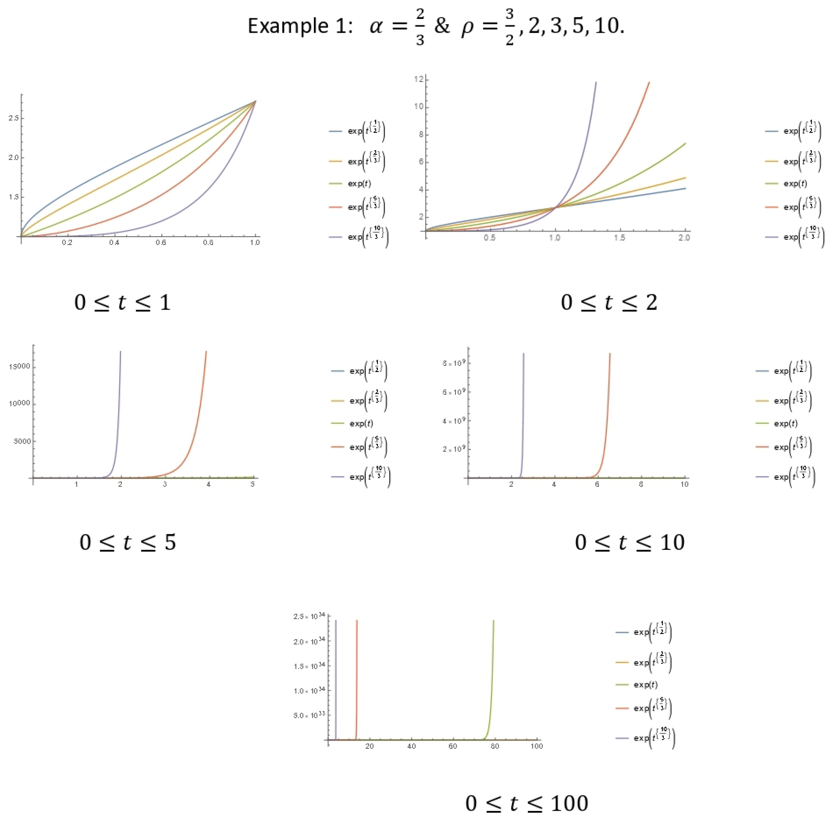
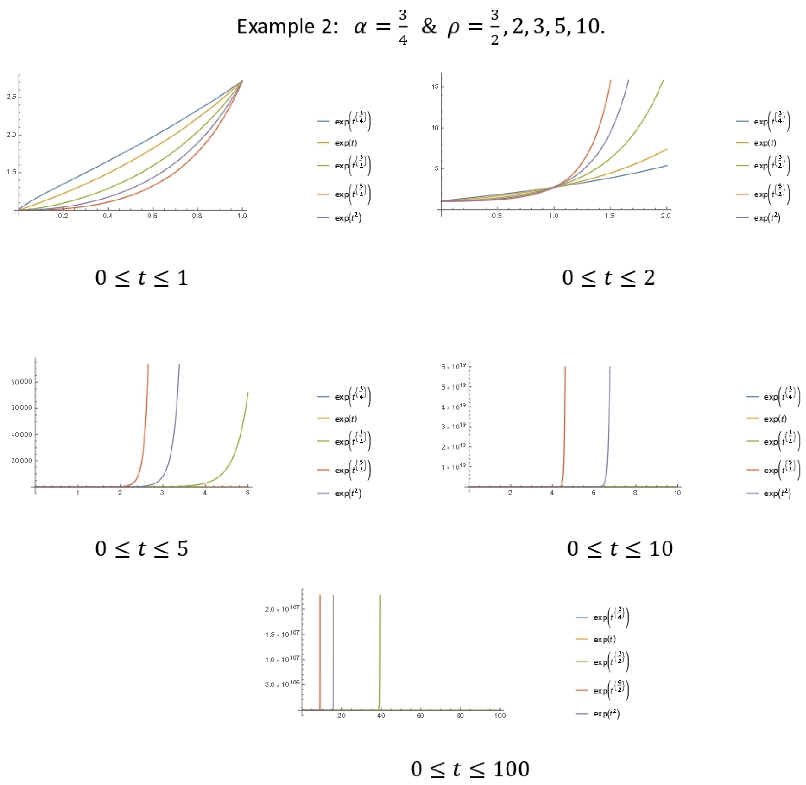
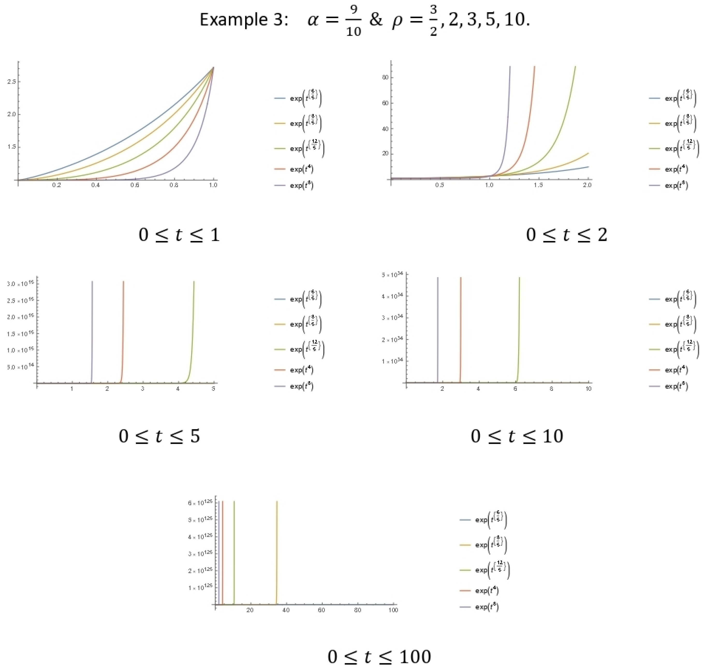
Additionally, we give examples to illustrate the result in Theorem 5, which represent plots (graphs) for the upper bound growth of our energy solution. For convenience, we set the positive constants to be equal to one. That is, $c_1={\tilde{c}}_{\alpha ,\rho }={\kappa }^2={\mathrm{Lip}}_{\vartheta }^2=1$ to have

$${\mathbf{E}\left|\phi \left(t\right)\right|}^2\le exp\left(t^{\rho (2\alpha -1)}\right),t\in [0,T],$$

where $\alpha \in (\frac{1}{2},1]$ and $\rho >1$.

• In Figure 1, we consider $\alpha =\frac{2}{3}$ and $\rho =\frac{3}{2},2,3,5,10$;
• Next, in Figure 2, we consider $\alpha =\frac{3}{4}$ and $\rho =\frac{3}{2},2,3,5,10$;
• Lastly, in Figure 3, we consider $\alpha =\frac{9}{10}$ and $\rho =\frac{3}{2},2,3,5,10$:

We observe that the values of $\alpha \in (\frac{1}{2},1)$ and $\rho \in (1,\infty )$ have little or no significant effect on the growth of the upper bound, however, as time t becomes large, the speed (rate) of growth becomes very sharp and fast. See the figures below.

4. Conclusions

The result suggests that lack of stringent enforcement of government policies, lack of adherence to public health policies (such as refusal to wear face-masks and non-compliance with social distancing) and rejection of vaccines administration, help in the spread (growth) of the infectious (COVID-19) disease. Mathematically put, the result investigated the properties of a class of Caputo–Katugampola stochastic fractional differential equation. Consequently, we estimated the upper growth bound of the random solution to the equation and showed that the energy solution grows exponentially at most at a precise rate. Banach fixed point theorem was applied to establish the existence and uniqueness result of the solution. We also noted that the solution exhibits some long time asymptotic behaviours. In the future, one can research on the lower bound estimate, stability and continuous dependence of the solution on the initial condition.

References

1. Foondun, M.; Liu, W.; Tian, K. Moment bounds for a class of Fractional Stochastic Heat Equations. Ann. Probab. 2017, 45, 2131–2153. [Google Scholar] [CrossRef] [Green Version]
2. Foondun, M.; Liu, W.; Omaba, M.E. On Some Properties of a class of Fractional Stochastic Heat Equations. J. Theoret. Probab. 2017, 30, 1310–1333. [Google Scholar]
3. Foondun, M.; Nane, E. Asymptotic properties of some space-time fractional stochastic equations. Math. Z. 2017, 287, 493–519. [Google Scholar] [CrossRef] [Green Version]
4. Foondun, M.; Liu, W.; Nane, E. Some non-existence results for a class of stochastic partial differential equations. J. Differ. Equ. 2019, 266, 2575–2596. [Google Scholar] [CrossRef] [Green Version]
5. Mijena, J.; Nane, E. Space-time fractional stochastic partial differential equations. Stoch. Process. Appl. 2015, 159, 3301–3326. [Google Scholar] [CrossRef]
6. Nane, E.; Nwaeze, E.R.; Omaba, M.E. Asymptotic behavior and non-existence of global solution to a class of conformable time-fractional stochastic differential equation. Stat. Probab. Lett. 2020, 163, 108792. [Google Scholar] [CrossRef] [Green Version]
7. Omaba, M.E.; Nwaeze, E.R. Moment Bound of Solution to a Class of Conformable Time-Fractional Stochastic Equation. Fractal Fract. 2019, 3, 18. [Google Scholar] [CrossRef] [Green Version]
8. Omaba, M.E. On a mild solution to hilfer time-fractional stochastic differetial equation. J. Fract. Calc. Appl. 2021, 12, 1–10. [Google Scholar]
9. Omaba, M.E.; Enyi, C.D. Atangana-Baleanu time-fractional stochastic integro-differential equation. Partial. Differ. Equ. Appl. Math. 2021, 4, 100100. [Google Scholar] [CrossRef]
10. Sakthivel, R.; Revathi, P.; Ren, Y. Existence of solutions for nonlinear fractional stochastic differential equations. Nonlinear Anal. 2013, 81, 70–86. [Google Scholar] [CrossRef]
11. Almeida, R.; Malinowska, A.B.; Odzijewicz, T. Fractional differential equations with dependence on the Caputo–Katugampola derivative. J. Comput. Nonlinear Dynam. 2016, 11, 061017. [Google Scholar] [CrossRef] [Green Version]
12. Katugampola, U.N. New approach to a generalized fractional integral. Appl. Math. Comput. 2011, 218, 860–865. [Google Scholar] [CrossRef] [Green Version]
13. Katugampola, U.N. A new approach to generalized fractional derivatives. Bull. Math. Anal. Appl. 2014, 6, 1–15. [Google Scholar]
14. Jarad, F.; Ugurlu, E.; Abdeljawad, T.; Baleanu, D. On a new class of fractional operators. Adv. Differ. Equ. 2017, 2017, 247. [Google Scholar] [CrossRef]
15. Jarad, F.; Abdeljawad, T.; Baleanu, D. On the generalized fractional derivatives and their Caputo modification. J. Nonlinear Sci. Appl. 2017, 10, 2607–2619. [Google Scholar] [CrossRef] [Green Version]
16. Katugampola, U.N. Existence and uniqueness results for a class of generalized fractional differential equations. arXiv 2014, arXiv:1411.5229. [Google Scholar]
17. Basti, B.; Arioua, Y.; Benhamidouche, N. Existence and uniqueness of solutions for nonlinear Katugampola fractional differential equations. J. Math. Appl. 2019, 42, 35–61. [Google Scholar] [CrossRef]
18. Basti, B.; Hammami, N.; Berrabah, I.; Nouioua, F.; Djemiat, R.; Benhamidouche, N. Stability Analysis and Existence of solutions for a Modified SIRD Model of COVID-19 with fractional derivatives. Symmetry 2021, 13, 1431. [Google Scholar] [CrossRef]
19. Rezapour, S.; Deressa, C.T.; Hussain, A.; Etemad, S.; George, R.; Ahmad, B. A Theoretical Analysis of a Fractional Multi-dimensional system of boundary value problems on the Methylpropane Graph via Fixed Point Technique. Mathematics 2022, 10, 568. [Google Scholar] [CrossRef]
20. Rashid, S.; Ashraf, R.; Bonyah, E. On Analytical solution of Time-fractional Biological population model by means of Generalized Integral Transform with their Uniqueness and Convergence Analysis. Adv. Nonlinear Anal. Appl. 2022, 2022, 7021288. [Google Scholar] [CrossRef]
21. Sintunavarat, W.; Turab, A. Mathematical analysis of an extended SEIR model of COVID-19 using the ABC-fractional operator. Math. Comput. Simul. 2022, 198, 65–84. [Google Scholar] [CrossRef] [PubMed]
22. Gambo, Y.Y.; Jarad, F.; Baleanu, D.; Abdeljawad, T. On Caputo modification of the Hadamard fractional derivatives. Adv. Differ. Equ. 2014, 2014, 10. [Google Scholar] [CrossRef] [Green Version]
23. Jarad, F.; Abdeljawad, T.; Baleanu, D. Caputo-type modification of the Hadamard fractional derivatives. Adv. Differ. Equ. 2012, 2012, 142. [Google Scholar] [CrossRef] [Green Version]
24. Lipovan, O. A retarded Gronwall-Like Inequality and Its Applications. J. Math. Anal. Appl. 2000, 252, 389–401. [Google Scholar] [CrossRef] [Green Version]
Figure 1. Graphical illustration of the energy growth bounds.
Mathematics 10 02086 g001
Figure 2. Graphical illustration of the energy growth bounds.
Mathematics 10 02086 g002
Figure 3. Graphical illustration of the energy growth bounds.
Mathematics 10 02086 g003
Publisher’s Note: MDPI stays neutral with regard to jurisdictional claims in published maps and institutional affiliations.