
An Adaptive EWMA Control Chart Based on Principal Component Method to Monitor Process Mean Vector

 ,
,
Abstract
:1. Introduction
2. Existing Methods
2.1. Process Characteristic
2.2. Mahalanobis Distance Statistic
2.3. Hotelling’s Control Chart
2.4. MC1 Control Chart
2.5. Control Chart Based on PCA
2.6. MC1PCA Control Chart
2.7. Relation between PCM and MD
2.8. Directional Invariance Property
3. Proposed Control Charts
3.1. Proposed Control Charts
3.2. Proposed Control Charts
3.3. Special Cases of Proposed and Control Charts
3.3.1. MCE(2) Control Chart Is a Special of Proposed Control Chart
3.3.2. MC1PCA Control Chart Is a Special of Proposed Control Chart
4. Performance Evaluation
4.1. Average Run Length
4.2. Overall Performance Measures
4.2.1. Extra Quadratic Loss
4.2.2. Relative Average Run Length
4.2.3. Performance Comparison Index
4.3. Choices of Parameters
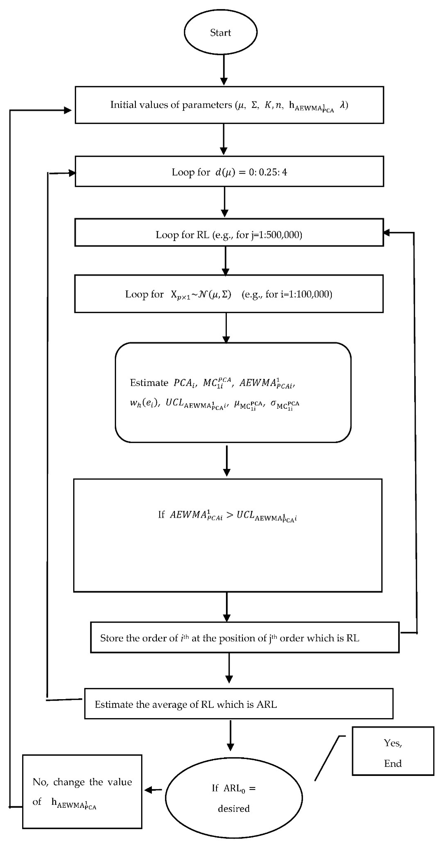
4.4. Construction of Proposed and Control Charts
- (i)
- Observations are drawn randomly from ( when ;
- (ii)
- The statistic is calculated from Equation (5) using and considering and PCs along their respective eigenvectors (i.e., ) and eigenvalues (i.e.,);
- (iii)
- Estimate the statistic from Equation (6) based on the statistic, constant , and , while is ;
- (iv)
- Calculate the statistic by using time varying and the statistic;
- (v)
- Let us assume that ;
- (vi)
- Computed the control limit from Equation (8), whereas the and are time-varying mean and standard deviation of the statistic, respectively calculated by empirical method;
- (vii)
- Plot the statistic against the control limit ; if the is true, the process is declared out of control, and the index of run length (RL) is recorded;
- (viii)
- Repeat from step (i) to step (vii) for 105 times to generate RLs and calculate their average, which is called ;
- (ix)
- If the is the targeted one, stop here; otherwise, change the value of accordingly in step (v) and repeat the process (i.e., step (i) to step (viii)) until the desired is achieved;
- (x)
- After obtaining the desired value of , consider and repeat steps from (i) to (ix) to obtain values.
4.5. Monte Carlo Simulation Procedure
5. Results and Discussion
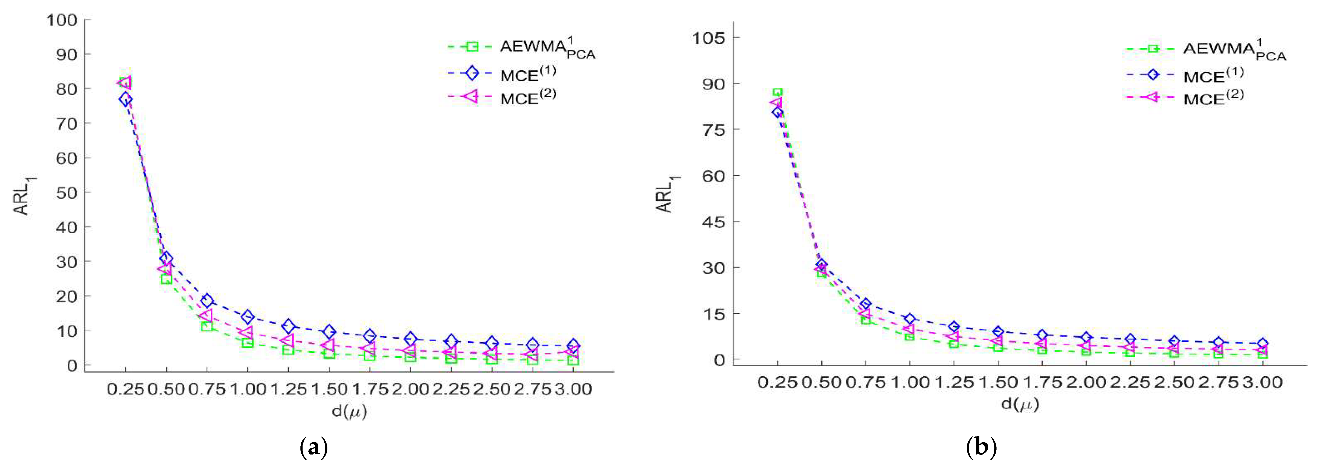
5.1. Proposed vs. and Control Charts
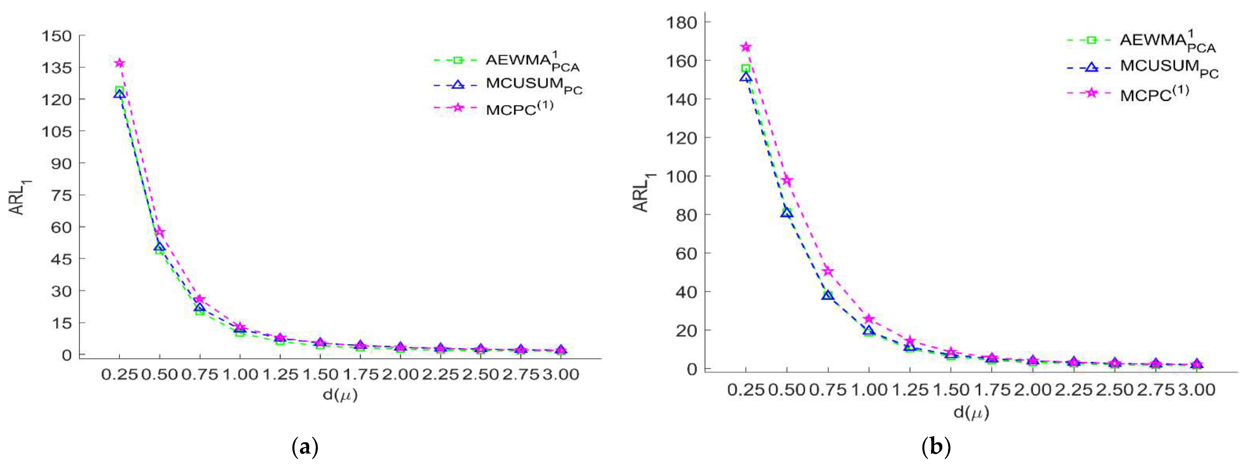
5.2. Proposed vs. Control Chart
5.3. Proposed vs. Control Chart
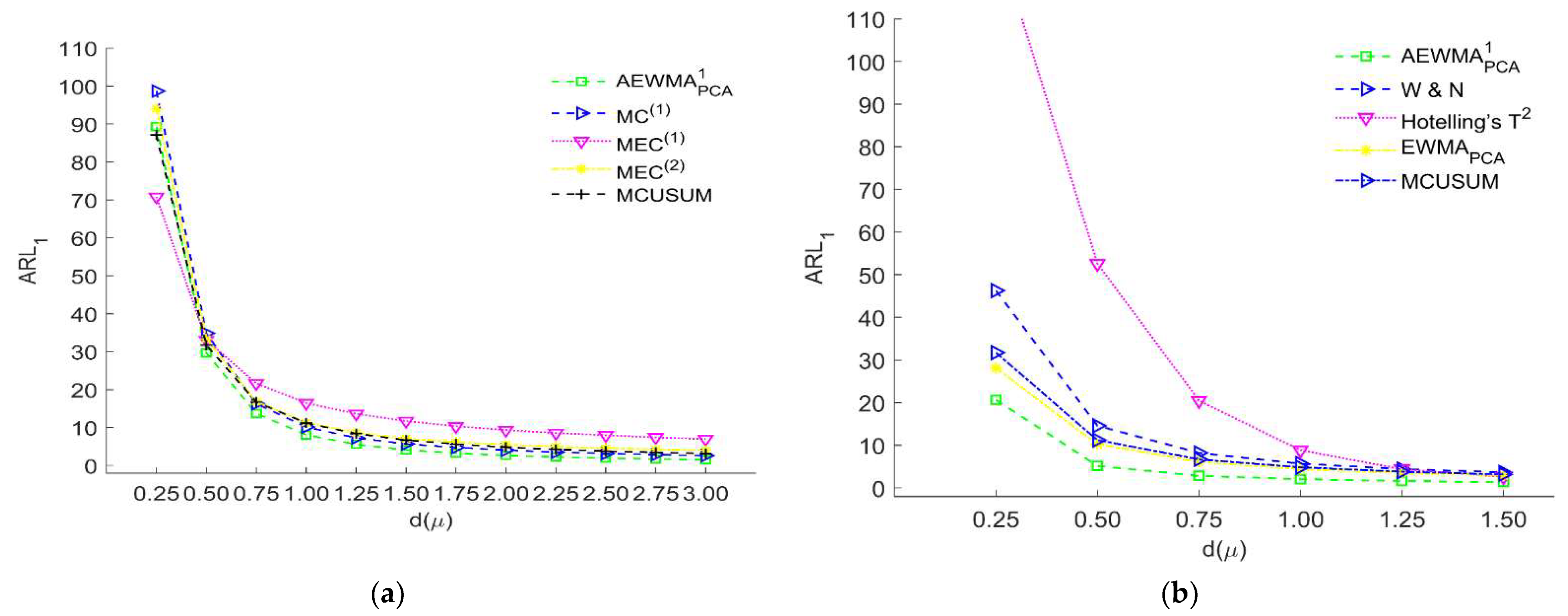
5.4. Proposed vs. and Control Charts
5.5. Proposed vs. Other Control Charts
6. Real-Life Example
7. Summary, Conclusions, and Recommendations
Author Contributions
Funding
Institutional Review Board Statement
Informed Consent Statement
Data Availability Statement
Acknowledgments
Conflicts of Interest
Abbreviations
| Acronym/Symbol | Description |
| ARL | Average Run Length |
| ARL0 | Out-of-Control Average Run Length |
| ARL1 | In-Control ARL0 |
| ARL1 and/or ARL0 at Specific Value of | |
| ARL1 and/or ARL0 at Specific Value of of a Benchmark Control Chart | |
| ACUSUM | Adaptive CUSUM |
| AEWMA | Adaptive EWMA (AEWMA) |
| Proposed Control Charts | |
| Based on Huber | |
| Based on Bi-square | |
| CUSUM | Cumulative Sum |
| Covariance | |
| Non-Centrality Parameter | |
| EQL | Extra Quadratic Loss |
| EWMA | Exponentially Weighted Moving Average |
| Eigenvectors of | |
| Error | |
| Plotting Statistic of EWMA | |
| Null Hypothesis | |
| Alternative Hypothesis | |
| Control Chart | |
| Control Chart | |
| control chart | |
| i | Sample of jth Quality Characteristic |
| Number of Quality Characteristic | |
| K/k | Constant |
| UCL | Upper Control Limit |
| Control Chart | |
| UCL of | |
| UCL of PC-chart | |
| MC1 | MCUSUM |
| UCL of | |
| MCUSUM | Multivariate CUSUM |
| MEWMA | Multivariate EWMA |
| MD | Mahalanobis Distance |
| Plotting Statistic of MC1 | |
| Control Chart Based on PCA | |
| Control Chart | |
| ni | Time Varying Sample |
| PCA | Principal Component Analysis |
| Plotting Statistic of PC-Chart | |
| PCI | Performance Comparison Index |
| Relative Average Run Length | |
| Constant | |
| or | Eigenvalues of |
| SDRL | Standard Deviation of RL |
| SERL | Standard Error of RL |
| SPC | Statistical Process Control |
| Chi-square Distribution | |
| / | Process Variables |
| ,, …, | Principal Components |
| Huber function | |
| Bi-square function | |
| Constant and | |
| Mean Vector | |
| Variance-Covariance Matrix | |
| Empirical Time Varying | |
| Empirical Time Varying |
References
- Montgomery, D.C. Introduction to Statistical Quality Control, 7th ed.; John Wiley & Sons: Hoboken, NJ, USA, 2012. [Google Scholar]
- Shewhart, W.A. Economic Control of Quality of Manufactured Product; D. Van Nostrand Company, Inc.: New York, NY, USA, 1931. [Google Scholar]
- Page, E. Continuous inspection schemes. Biometrika 1954, 41, 100–115. [Google Scholar] [CrossRef]
- Roberts, S. Control chart tests based on geometric moving averages. Technometrics 1959, 1, 239–250. [Google Scholar] [CrossRef]
- Hotelling, H. Multivariate quality control, illustrated by the air testing of sample bombsights. In Techniques of Statistical Analysis; McGraw Hill: New York, NY, USA, 1947; pp. 111–184. [Google Scholar]
- Woodall, W.H.; Ncube, M.M. Multivariate CUSUM quality-control procedures. Technometrics 1985, 27, 285–292. [Google Scholar] [CrossRef]
- Crosier, R.B. Multivariate generalizations of cumulative sum quality-control schemes. Technometrics 1988, 30, 291–303. [Google Scholar] [CrossRef]
- Pignatiello, J.J., Jr.; Runger, G.C. Comparisons of multivariate CUSUM charts. J. Qual. Technol. 1990, 22, 173–186. [Google Scholar] [CrossRef]
- Lowry, C.A.; Woodall, W.H.; Champ, C.W.; Rigdon, S.E. A multivariate exponentially weighted moving average control chart. Technometrics 1992, 34, 46–53. [Google Scholar] [CrossRef]
- Johnson, R.; Wichern, D. Applied Statistical Multivariate Analysis; Prentice-Hall: Upper Saddle River, NJ, USA, 2002. [Google Scholar]
- Varmuza, K.; Filzmoser, P. Introduction to Multivariate Statistical Analysis in Chemometrics; CRC press: Boca Raton, FL, USA, 2016. [Google Scholar]
- Zaman, B.; Lee, M.H.; Riaz, M. An improved process monitoring by mixed multivariate memory control charts: An application in wind turbine field. Comput. Ind. Eng. 2020, 142, 106343. [Google Scholar] [CrossRef]
- Aït-Sahalia, Y.; Xiu, D. Principal component analysis of high-frequency data. J. Am. Stat. Assoc. 2019, 114, 287–303. [Google Scholar] [CrossRef]
- Scranton, R.; Runger, G.C.; Keats, J.B.; Montgomery, D.C. Efficient shift detection using multivariate exponentially-weighted moving average control charts and principal components. Qual. Reliab. Eng. Int. 1996, 12, 165–171. [Google Scholar] [CrossRef]
- Jackson, J.E.; Morris, R.H. An application of multivariate quality control to photographic processing. J. Am. Stat. Assoc. 1957, 52, 186–199. [Google Scholar] [CrossRef]
- Wold, S. Exponentially weighted moving principal components analysis and projections to latent structures. Chemom. Intell. Lab. Syst. 1994, 23, 149–161. [Google Scholar] [CrossRef]
- Zou, C.; Zhou, C.; Wang, Z.; Tsung, F. A self-starting control chart for linear profiles. J. Qual. Technol. 2007, 39, 364–375. [Google Scholar] [CrossRef]
- Zou, C.; Tsung, F.; Wang, Z. Monitoring general linear profiles using multivariate exponentially weighted moving average schemes. Technometrics 2007, 49, 395–408. [Google Scholar] [CrossRef]
- Jackson, J.E. Principal components and factor analysis: Part II—Additional topics related to principal components. J. Qual. Technol. 1981, 13, 46–58. [Google Scholar] [CrossRef]
- Jackson, J.E. Principal Components and Factor Analysis: Part III—What is Factor Analysis? J. Qual. Technol. 1981, 13, 125–130. [Google Scholar] [CrossRef]
- Machado, M.A.; Costa, A.F. The use of principal components and univariate charts to control multivariate processes. Pesquisa Operacional 2008, 28, 173–196. [Google Scholar] [CrossRef]
- Yue, J.; Liu, L. Multivariate nonparametric control chart with variable sampling interval. Appl. Math. Model. 2017, 52, 603–612. [Google Scholar] [CrossRef]
- Riaz, M.; Zaman, B.; Mehmood, R.; Abbas, N.; Abujiya, M. Advanced multivariate cumulative sum control charts based on principal component method with application. Qual. Reliab. Eng. Int. 2021, 37, 2760–2789. [Google Scholar] [CrossRef]
- Hawkins, D.M.; Wu, Q.F. The CUSUM and the EWMA Head-to-Head. Qual. Eng. 2014, 26, 215–222. [Google Scholar] [CrossRef]
- Sparks, R.S. CUSUM charts for signalling varying location shifts. J. Qual. Technol. 2000, 32, 157–171. [Google Scholar] [CrossRef]
- Capizzi, G.; Masarotto, G. An adaptive exponentially weighted moving average control chart. Technometrics 2003, 45, 199–207. [Google Scholar] [CrossRef]
- Jiang, W.; Shu, L.; Apley, D.W. Adaptive CUSUM procedures with EWMA-based shift estimators. IIE Trans. 2008, 40, 992–1003. [Google Scholar] [CrossRef]
- Wu, Z.; Jiao, J.X.; Yang, M.; Liu, Y.; Wang, Z.J. An enhanced adaptive Cusum control chart. IIE Trans. 2009, 41, 642–653. [Google Scholar] [CrossRef]
- Haq, A.; Gulzar, R.; Khoo, M.B. An efficient adaptive EWMA control chart for monitoring the process mean. Qual. Reliab. Eng. Int. 2018, 34, 563–571. [Google Scholar] [CrossRef]
- Jiao, J.R.; Helo, P.T. Optimization design of a CUSUM control chart based on Taguchi’s loss function. Int. J. Adv. Manuf. Technol. 2008, 35, 1234–1243. [Google Scholar] [CrossRef]
- Zaman, B.; Lee, M.H.; Riaz, M. An adaptive EWMA Chart with CUSUM accumulate error-based shift estimator for efficient process dispersion monitoring. Comput. Ind. Eng. 2019, 135, 236–253. [Google Scholar] [CrossRef]
- Zaman, B.; Lee, M.H.; Riaz, M.; Abujiya, M.R. An adaptive EWMA scheme-based CUSUM accumulation error for efficient monitoring of process location. Qual. Reliab. Eng. Int. 2017, 33, 2463–2482. [Google Scholar] [CrossRef]
- Zaman, B.; Lee, M.H.; Riaz, M.; Abujiya, M.R. An adaptive approach to EWMA dispersion chart using Huber and Tukey functions. Qual. Reliab. Eng. Int. 2019, 35, 1542–1581. [Google Scholar] [CrossRef]
- Amiri, A.; Nedaie, A.; Alikhani, M. A new adaptive variable sample size approach in EWMA control chart. Commun. Stat. -Simul. Comput. 2014, 43, 804–812. [Google Scholar] [CrossRef]
- Chatterjee, S.; Qiu, P. Distribution-free cumulative sum control charts using bootstrap-based control limits. Ann. Appl. Stat. 2009, 3, 349–369. [Google Scholar] [CrossRef]
- Hawkins, D.M.; Zamba, K. On small shifts in quality control. Qual. Eng. 2003, 16, 143–149. [Google Scholar] [CrossRef]
- Hussain, S.; Song, L.-x.; Ahmad, S.; Riaz, M. A new auxiliary information based cumulative sum median control chart for location monitoring. Front. Inf. Technol. Electron. Eng. 2019, 20, 554–570. [Google Scholar] [CrossRef]
- Khoo, M.B. Determining the time of a permanent shift in the process mean of CUSUM control charts. Qual. Eng. 2004, 17, 87–93. [Google Scholar] [CrossRef]
- Khoo, M.B.; Teh, S. A Study on the Effects of Trends due to Inertia on EWMA and CUSUM Charts. J. Qual. Meas. Anal. 2009, 5, 73–80. [Google Scholar]
- Liu, L.; Zi, X.; Zhang, J.; Wang, Z. A sequential rank-based nonparametric adaptive EWMA control chart. Commun. Stat.-Simul. Comput. 2013, 42, 841–859. [Google Scholar] [CrossRef]
- Luceño, A.; Puig-Pey, J. Evaluation of the run-length probability distribution for CUSUM charts: Assessing chart performance. Technometrics 2000, 42, 411–416. [Google Scholar]
- Maravelakis, P.E. Measurement error effect on the CUSUM control chart. J. Appl. Stat. 2012, 39, 323–336. [Google Scholar] [CrossRef]
- Ou, Y.; Wu, Z.; Lee, K.M.; Wu, K. An adaptive CUSUM chart with single sample size for monitoring process mean and variance. Qual. Reliab. Eng. Int. 2013, 29, 1027–1039. [Google Scholar] [CrossRef]
- Zaman, B.; Riaz, M.; Abbas, N.; Does, R. Mixed Cumulative Sum-Exponentially Weighted Moving Average Control Charts: An Efficient Way of Monitoring Process Location. Qual. Reliab. Eng. Int. 2015, 31, 1407–1421. [Google Scholar] [CrossRef]
- Zhao, Y.; Tsung, F.; Wang, Z. Dual CUSUM control schemes for detecting a range of mean shifts. IIE Trans. 2005, 37, 1047–1057. [Google Scholar] [CrossRef]
- Mahalanobis, P.C. On the Generalized Distance in Statistics; National Institute of Science of India: Jatani, India, 1936. [Google Scholar]
- Kumar, S.; Chow, T.W.; Pecht, M. Approach to fault identification for electronic products using Mahalanobis distance. IEEE Trans. Instrum. Meas. 2009, 59, 2055–2064. [Google Scholar] [CrossRef]
- Ranger, G.C.; Alt, F.B. Choosing principal components for multivariate statistical process control. Commun. Stat.-Theory Methods 1996, 25, 909–922. [Google Scholar] [CrossRef]
- Mehmood, R.; Lee, M.H.; Riaz, M.; Zaman, B.; Ali, I. Hotelling T 2 control chart based on bivariate ranked set schemes. Commun. Stat. Simul. Comput. 2019, 51, 1–28. [Google Scholar]
- Abbas, N.; Saeed, U.; Riaz, M. Assorted control charts: An efficient statistical approach to monitor pH values in ecotoxicology lab. J. Chemom. 2019, 33, e3129. [Google Scholar] [CrossRef]
- Chen, R.; Li, Z.; Zhang, J. A generally weighted moving average control chart for monitoring the coefficient of variation. Appl. Math. Model. 2019, 70, 190–205. [Google Scholar] [CrossRef]
- Riaz, M.; Abbasi, S.A.; Ahmad, S.; Zaman, B. On efficient phase II process monitoring charts. Int. J. Adv. Manuf. Technol. 2014, 70, 2263–2274. [Google Scholar] [CrossRef]
- Ou, Y.; Wu, Z.; Goh, T.N. A new SPRT chart for monitoring process mean and variance. Int. J. Prod. Econ. 2011, 132, 303–314. [Google Scholar] [CrossRef]
- Luo, Y.; Li, Z.; Wang, Z. Adaptive CUSUM control chart with variable sampling intervals. Comput. Stat. Data Anal. 2009, 53, 2693–2701. [Google Scholar] [CrossRef]
- Zaman, B.; Abbas, N.; Riaz, M.; Lee, M.H. Mixed CUSUM-EWMA chart for monitoring process dispersion. Int. J. Adv. Manuf. Technol. 2016, 86, 3025–3039. [Google Scholar]
- Ajadi, J.O.; Riaz, M. Mixed multivariate EWMA-CUSUM control charts for an improved process monitoring. Commun. Stat.-Theory Methods 2017, 46, 6980–6993. [Google Scholar] [CrossRef]


| 0.05 | 0.05 | 0.05 | 0.05 | 0.05 | 0.05 | 0.05 | 0.10 | 0.10 | 0.10 | 0.10 | 0.10 | 0.10 | 0.10 | ||
| 1.00 | 1.50 | 2.00 | 2.50 | 3.00 | 3.50 | 4.00 | 1.00 | 1.50 | 2.00 | 2.50 | 3.00 | 3.50 | 4.00 | ||
| 17.52 | 15.22 | 12.82 | 9.02 | 5.42 | 4.02 | 3.58 | 11.28 | 10.52 | 10.18 | 6.18 | 4.98 | 4.48 | 4.28 | ||
| 0.00 | ARL | 197 | 198.71 | 200 | 205 | 200 | 202 | 205.38 | 200 | 206.368 | 198 | 202 | 202 | 200 | 198 |
| SDRL | 225 | 224 | 213 | 214.74 | 203 | 195 | 191 | 214 | 212 | 205.26 | 201.63 | 199 | 193 | 187 | |
| SERL | 1.593 | 1.585 | 1.509 | 1.518 | 1.433 | 1.378 | 1.353 | 1.516 | 1.501 | 1.451 | 1.426 | 1.409 | 1.368 | 1.324 | |
| 0.25 | ARL | 81.79 | 84.60 | 87.28 | 89.07 | 86.44 | 86.19 | 88.40 | 87.16 | 90.3022 | 88.72 | 88.34 | 87.26 | 85.34 | 84.73 |
| SDRL | 94.24 | 94.13 | 90.86 | 92.37 | 84.70 | 78.04 | 76.23 | 91.58 | 91.93 | 90.77 | 87.43 | 82.29 | 77.78 | 76.95 | |
| SERL | 0.666 | 0.666 | 0.642 | 0.653 | 0.599 | 0.552 | 0.539 | 0.648 | 0.650 | 0.642 | 0.618 | 0.582 | 0.550 | 0.544 | |
| 0.50 | ARL | 24.87 | 26.42 | 27.55 | 28.44 | 29.00 | 30.15 | 31.42 | 27.89 | 29.1529 | 29.67 | 29.65 | 30.08 | 30.20 | 30.12 |
| SDRL | 26.46 | 26.27 | 26.56 | 26.05 | 24.74 | 23.23 | 23.05 | 26.88 | 27.41 | 26.95 | 25.45 | 24.20 | 23.15 | 22.61 | |
| SERL | 0.187 | 0.186 | 0.188 | 0.184 | 0.175 | 0.164 | 0.163 | 0.190 | 0.194 | 0.191 | 0.180 | 0.171 | 0.164 | 0.160 | |
| 0.75 | ARL | 11.10 | 12.05 | 12.73 | 13.33 | 14.14 | 14.91 | 16.16 | 12.66 | 13.1558 | 13.65 | 14.21 | 14.87 | 15.16 | 15.49 |
| SDRL | 10.14 | 9.97 | 9.91 | 10.09 | 10.08 | 9.69 | 9.68 | 10.68 | 10.44 | 10.54 | 10.49 | 10.09 | 9.38 | 9.07 | |
| SERL | 0.072 | 0.071 | 0.070 | 0.071 | 0.071 | 0.069 | 0.068 | 0.076 | 0.074 | 0.075 | 0.074 | 0.071 | 0.066 | 0.064 | |
| 1.00 | ARL | 6.37 | 7.12 | 7.64 | 8.09 | 8.57 | 9.33 | 10.17 | 7.28 | 7.7447 | 8.16 | 8.50 | 9.06 | 9.65 | 10.14 |
| SDRL | 5.13 | 5.09 | 5.15 | 5.02 | 5.10 | 5.23 | 5.36 | 5.58 | 5.31 | 5.36 | 5.32 | 5.24 | 5.04 | 4.96 | |
| SERL | 0.036 | 0.036 | 0.037 | 0.036 | 0.036 | 0.037 | 0.038 | 0.040 | 0.038 | 0.038 | 0.038 | 0.037 | 0.036 | 0.035 | |
| 1.25 | ARL | 4.36 | 4.94 | 5.37 | 5.68 | 6.07 | 6.64 | 7.31 | 4.92 | 5.3273 | 5.65 | 6.00 | 6.46 | 6.99 | 7.48 |
| SDRL | 3.11 | 3.10 | 3.07 | 3.06 | 3.14 | 3.24 | 3.38 | 3.35 | 3.23 | 3.23 | 3.24 | 3.30 | 3.30 | 3.24 | |
| SERL | 0.022 | 0.022 | 0.022 | 0.022 | 0.022 | 0.023 | 0.024 | 0.024 | 0.023 | 0.023 | 0.023 | 0.023 | 0.023 | 0.023 | |
| 1.50 | ARL | 3.26 | 3.74 | 4.14 | 4.41 | 4.69 | 5.12 | 5.63 | 3.66 | 4.0312 | 4.29 | 4.57 | 4.95 | 5.39 | 5.82 |
| SDRL | 2.06 | 2.10 | 2.10 | 2.10 | 2.13 | 2.24 | 2.34 | 2.29 | 2.24 | 2.18 | 2.20 | 2.27 | 2.32 | 2.32 | |
| SERL | 0.015 | 0.015 | 0.015 | 0.015 | 0.015 | 0.016 | 0.017 | 0.016 | 0.016 | 0.015 | 0.016 | 0.016 | 0.016 | 0.016 | |
| 1.75 | ARL | 2.63 | 3.02 | 3.37 | 3.60 | 3.86 | 4.22 | 4.58 | 2.90 | 3.215 | 3.46 | 3.71 | 4.00 | 4.38 | 4.76 |
| SDRL | 1.50 | 1.52 | 1.54 | 1.54 | 1.58 | 1.62 | 1.72 | 1.66 | 1.65 | 1.61 | 1.63 | 1.66 | 1.72 | 1.76 | |
| SERL | 0.011 | 0.011 | 0.011 | 0.011 | 0.011 | 0.012 | 0.012 | 0.012 | 0.012 | 0.011 | 0.012 | 0.012 | 0.012 | 0.012 | |
| 2.00 | ARL | 2.20 | 2.54 | 2.84 | 3.06 | 3.25 | 3.56 | 3.88 | 2.39 | 2.6923 | 2.89 | 3.12 | 3.36 | 3.67 | 3.99 |
| SDRL | 1.15 | 1.17 | 1.20 | 1.21 | 1.21 | 1.28 | 1.32 | 1.26 | 1.26 | 1.25 | 1.26 | 1.29 | 1.34 | 1.38 | |
| SERL | 0.008 | 0.008 | 0.009 | 0.009 | 0.009 | 0.009 | 0.009 | 0.009 | 0.009 | 0.009 | 0.009 | 0.009 | 0.010 | 0.010 | |
| 2.25 | ARL | 1.90 | 2.19 | 2.46 | 2.67 | 2.85 | 3.09 | 3.37 | 2.03 | 2.3018 | 2.52 | 2.69 | 2.92 | 3.18 | 3.46 |
| SDRL | 0.92 | 0.97 | 0.97 | 0.99 | 0.99 | 1.01 | 1.07 | 1.00 | 1.02 | 1.02 | 1.02 | 1.04 | 1.08 | 1.12 | |
| SERL | 0.007 | 0.007 | 0.007 | 0.007 | 0.007 | 0.007 | 0.008 | 0.007 | 0.007 | 0.007 | 0.007 | 0.007 | 0.008 | 0.008 | |
| 2.50 | ARL | 1.66 | 1.93 | 2.18 | 2.37 | 2.53 | 2.75 | 3.00 | 1.78 | 2.0204 | 2.21 | 2.39 | 2.58 | 2.80 | 3.05 |
| SDRL | 0.75 | 0.81 | 0.82 | 0.82 | 0.83 | 0.85 | 0.90 | 0.82 | 0.86 | 0.86 | 0.86 | 0.86 | 0.88 | 0.93 | |
| SERL | 0.005 | 0.006 | 0.006 | 0.006 | 0.006 | 0.006 | 0.006 | 0.006 | 0.006 | 0.006 | 0.006 | 0.006 | 0.006 | 0.007 | |
| 2.75 | ARL | 1.49 | 1.74 | 1.95 | 2.12 | 2.29 | 2.49 | 2.70 | 1.59 | 1.8058 | 1.98 | 2.14 | 2.33 | 2.52 | 2.74 |
| SDRL | 0.65 | 0.71 | 0.72 | 0.71 | 0.71 | 0.72 | 0.76 | 0.70 | 0.74 | 0.75 | 0.73 | 0.74 | 0.75 | 0.80 | |
| SERL | 0.005 | 0.005 | 0.005 | 0.005 | 0.005 | 0.005 | 0.005 | 0.005 | 0.005 | 0.005 | 0.005 | 0.005 | 0.005 | 0.006 | |
| 3.00 | ARL | 1.37 | 1.57 | 1.77 | 1.95 | 2.11 | 2.28 | 2.46 | 1.44 | 1.6265 | 1.79 | 1.96 | 2.13 | 2.31 | 2.49 |
| SDRL | 0.56 | 0.63 | 0.65 | 0.63 | 0.62 | 0.63 | 0.66 | 0.60 | 0.66 | 0.67 | 0.66 | 0.66 | 0.65 | 0.69 | |
| SERL | 0.004 | 0.004 | 0.005 | 0.005 | 0.004 | 0.004 | 0.005 | 0.004 | 0.005 | 0.005 | 0.005 | 0.005 | 0.005 | 0.005 | |
| 4.00 | ARL | 1.08 | 1.17 | 1.29 | 1.43 | 1.59 | 1.76 | 1.92 | 1.10 | 1.1942 | 1.30 | 1.43 | 1.58 | 1.75 | 1.91 |
| SDRL | 0.27 | 0.38 | 0.46 | 0.51 | 0.52 | 0.49 | 0.44 | 0.30 | 0.40 | 0.47 | 0.51 | 0.52 | 0.49 | 0.46 | |
| SERL | 0.002 | 0.003 | 0.003 | 0.004 | 0.004 | 0.004 | 0.003 | 0.002 | 0.003 | 0.003 | 0.004 | 0.004 | 0.004 | 0.003 | |
| 5.00 | ARL | 1.01 | 1.02 | 1.06 | 1.12 | 1.20 | 1.35 | 1.54 | 1.01 | 1.0313 | 1.06 | 1.11 | 1.21 | 1.35 | 1.51 |
| SDRL | 0.09 | 0.15 | 0.24 | 0.33 | 0.40 | 0.48 | 0.50 | 0.10 | 0.17 | 0.24 | 0.32 | 0.41 | 0.48 | 0.50 | |
| SERL | 0.001 | 0.001 | 0.002 | 0.002 | 0.003 | 0.0034 | 0.004 | 0.001 | 0.001 | 0.0017 | 0.002 | 0.003 | 0.003 | 0.004 | |
| λ | 0.20 | 0.20 | 0.20 | 0.20 | 0.20 | 0.20 | 0.20 | 0.30 | 0.30 | 0.30 | 0.30 | 0.30 | 0.30 | 0.30 | |
| γ | 1.00 | 1.50 | 2.00 | 2.50 | 3.00 | 3.50 | 4.00 | 1.00 | 1.50 | 2.00 | 2.50 | 3.00 | 3.50 | 4.00 | |
| d(μ) | 7.58 | 6.68 | 5.68 | 5.28 | 4.70 | 4.65 | 4.6 | 5.93 | 5.33 | 4.85 | 4.59 | 4.49 | 4.42 | 4.42 | |
| 0.00 | ARL | 199 | 200 | 200 | 201 | 197 | 201 | 200 | 199 | 201 | 200 | 201 | 202 | 197 | 197 |
| SDRL | 207 | 203 | 203 | 198.75 | 195 | 196 | 194 | 203.64 | 201 | 201 | 198.41 | 199 | 193.8477 | 195 | |
| SERL | 1.465 | 1.433 | 1.434 | 1.405 | 1.377 | 1.388 | 1.373 | 1.440 | 1.423 | 1.425 | 1.403 | 1.409 | 1.371 | 1.381 | |
| 0.25 | ARL | 88.63 | 91 | 89.54 | 86.77 | 86 | 88.47 | 87.94 | 89.31 | 89.30 | 89.09 | 88.10 | 87.92 | 86.16 | 87.26 |
| SDRL | 88.68 | 90.19 | 88.68 | 82.19 | 81.27 | 83.46 | 81.51 | 90.10 | 86.70 | 85.80 | 84.22 | 83.88 | 82.4045 | 83.12 | |
| SERL | 0.627 | 0.638 | 0.627 | 0.581 | 0.575 | 0.590 | 0.576 | 0.637 | 0.613 | 0.607 | 0.596 | 0.593 | 0.583 | 0.588 | |
| 0.50 | ARL | 29.51 | 30.49 | 30.20 | 29.97 | 29.77 | 30.29 | 30.05 | 29.70 | 29.82 | 30.31 | 29.86 | 29.80 | 29.54 | 29.51 |
| SDRL | 26.73 | 27.41 | 26.18 | 25.13 | 24.61 | 24.24 | 23.54 | 26.73 | 26.04 | 25.57 | 24.70 | 24.41 | 24.1859 | 23.98 | |
| SERL | 0.189 | 0.194 | 0.185 | 0.178 | 0.174 | 0.171 | 0.166 | 0.189 | 0.184 | 0.181 | 0.175 | 0.173 | 0.171 | 0.170 | |
| 0.75 | ARL | 13.50 | 13.85 | 14.15 | 14.50 | 14.62 | 15.09 | 14.97 | 13.69 | 13.95 | 14.23 | 14.56 | 14.62 | 14.61 | 14.66 |
| SDRL | 10.58 | 10.57 | 10.40 | 10.04 | 9.52 | 9.58 | 9.41 | 10.62 | 10.44 | 10.18 | 10.01 | 9.88 | 9.593 | 9.86 | |
| SERL | 0.075 | 0.075 | 0.074 | 0.071 | 0.067 | 0.068 | 0.067 | 0.075 | 0.074 | 0.072 | 0.071 | 0.070 | 0.068 | 0.070 | |
| 1.00 | ARL | 7.99 | 8.29 | 8.54 | 8.96 | 9.30 | 9.60 | 9.66 | 8.04 | 8.37 | 8.69 | 8.93 | 9.17 | 9.16 | 9.25 |
| SDRL | 5.53 | 5.56 | 5.36 | 5.22 | 5.00 | 4.91 | 4.80 | 5.46 | 5.44 | 5.35 | 5.16 | 5.06 | 4.9861 | 4.95 | |
| SERL | 0.039 | 0.039 | 0.038 | 0.037 | 0.035 | 0.035 | 0.034 | 0.039 | 0.039 | 0.038 | 0.037 | 0.036 | 0.035 | 0.035 | |
| 1.25 | ARL | 5.40 | 5.64 | 5.93 | 6.30 | 6.67 | 7.05 | 7.18 | 5.58 | 5.79 | 6.10 | 6.39 | 6.61 | 6.70 | 6.79 |
| SDRL | 3.45 | 3.36 | 3.34 | 3.29 | 3.19 | 3.10 | 2.98 | 3.43 | 3.35 | 3.37 | 3.24 | 3.10 | 3.0321 | 3.01 | |
| SERL | 0.024 | 0.024 | 0.024 | 0.023 | 0.023 | 0.022 | 0.021 | 0.024 | 0.024 | 0.024 | 0.023 | 0.022 | 0.021 | 0.021 | |
| 1.50 | ARL | 4.03 | 4.23 | 4.53 | 4.83 | 5.22 | 5.53 | 5.78 | 4.11 | 4.34 | 4.62 | 4.90 | 5.16 | 5.31 | 5.36 |
| SDRL | 2.37 | 2.29 | 2.31 | 2.30 | 2.29 | 2.22 | 2.12 | 2.35 | 2.35 | 2.33 | 2.26 | 2.18 | 2.1094 | 2.03 | |
| SERL | 0.017 | 0.016 | 0.016 | 0.016 | 0.016 | 0.016 | 0.015 | 0.017 | 0.017 | 0.017 | 0.016 | 0.015 | 0.015 | 0.014 | |
| 1.75 | ARL | 3.15 | 3.40 | 3.60 | 3.89 | 4.20 | 4.52 | 4.79 | 3.27 | 3.46 | 3.71 | 3.97 | 4.21 | 4.39 | 4.51 |
| SDRL | 1.74 | 1.72 | 1.68 | 1.72 | 1.71 | 1.70 | 1.65 | 1.75 | 1.73 | 1.74 | 1.71 | 1.66 | 1.5854 | 1.55 | |
| SERL | 0.012 | 0.012 | 0.012 | 0.012 | 0.012 | 0.012 | 0.012 | 0.012 | 0.012 | 0.012 | 0.012 | 0.012 | 0.011 | 0.011 | |
| 2.00 | ARL | 2.60 | 2.80 | 2.99 | 3.26 | 3.54 | 3.85 | 4.08 | 2.68 | 2.87 | 3.07 | 3.32 | 3.58 | 3.77 | 3.87 |
| SDRL | 1.35 | 1.32 | 1.34 | 1.35 | 1.36 | 1.40 | 1.33 | 1.36 | 1.35 | 1.37 | 1.36 | 1.35 | 1.3002 | 1.23 | |
| SERL | 0.010 | 0.009 | 0.009 | 0.010 | 0.010 | 0.010 | 0.009 | 0.010 | 0.010 | 0.010 | 0.010 | 0.010 | 0.009 | 0.009 | |
| 2.25 | ARL | 2.20 | 2.39 | 2.58 | 2.78 | 3.05 | 3.31 | 3.54 | 2.27 | 2.44 | 2.62 | 2.84 | 3.07 | 3.26 | 3.41 |
| SDRL | 1.08 | 1.07 | 1.08 | 1.08 | 1.11 | 1.13 | 1.12 | 1.10 | 1.09 | 1.10 | 1.11 | 1.11 | 1.0782 | 1.04 | |
| SERL | 0.008 | 0.008 | 0.008 | 0.008 | 0.008 | 0.008 | 0.008 | 0.008 | 0.008 | 0.008 | 0.008 | 0.008 | 0.008 | 0.007 | |
| 2.50 | ARL | 1.91 | 2.09 | 2.25 | 2.45 | 2.66 | 2.91 | 3.13 | 1.96 | 2.10 | 2.29 | 2.49 | 2.70 | 2.89 | 3.04 |
| SDRL | 0.89 | 0.90 | 0.89 | 0.90 | 0.93 | 0.96 | 0.96 | 0.92 | 0.91 | 0.92 | 0.92 | 0.95 | 0.9405 | 0.89 | |
| SERL | 0.006 | 0.006 | 0.006 | 0.006 | 0.007 | 0.007 | 0.007 | 0.007 | 0.006 | 0.007 | 0.007 | 0.007 | 0.007 | 0.006 | |
| 2.75 | ARL | 1.69 | 1.85 | 2.01 | 2.19 | 2.39 | 2.61 | 2.81 | 1.73 | 1.88 | 2.03 | 2.23 | 2.40 | 2.60 | 2.74 |
| SDRL | 0.75 | 0.78 | 0.78 | 0.78 | 0.79 | 0.81 | 0.83 | 0.78 | 0.79 | 0.79 | 0.81 | 0.81 | 0.8078 | 0.78 | |
| SERL | 0.005 | 0.006 | 0.006 | 0.006 | 0.006 | 0.006 | 0.006 | 0.006 | 0.006 | 0.006 | 0.006 | 0.006 | 0.006 | 0.006 | |
| 3.00 | ARL | 1.52 | 1.68 | 1.82 | 1.97 | 2.17 | 2.37 | 2.53 | 1.56 | 1.68 | 1.83 | 1.99 | 2.18 | 2.34 | 2.49 |
| SDRL | 0.64 | 0.68 | 0.69 | 0.69 | 0.70 | 0.71 | 0.72 | 0.67 | 0.69 | 0.71 | 0.72 | 0.72 | 0.712 | 0.70 | |
| SERL | 0.005 | 0.005 | 0.005 | 0.005 | 0.005 | 0.005 | 0.005 | 0.005 | 0.005 | 0.005 | 0.005 | 0.005 | 0.005 | 0.005 | |
| 4.00 | ARL | 1.13 | 1.21 | 1.30 | 1.42 | 1.57 | 1.75 | 1.90 | 1.15 | 1.21 | 1.29 | 1.42 | 1.56 | 1.70 | 1.85 |
| SDRL | 0.35 | 0.42 | 0.47 | 0.51 | 0.54 | 0.52 | 0.49 | 0.36 | 0.42 | 0.47 | 0.52 | 0.54 | 0.5341 | 0.51 | |
| SERL | 0.002 | 0.003 | 0.003 | 0.004 | 0.004 | 0.004 | 0.004 | 0.003 | 0.003 | 0.003 | 0.004 | 0.004 | 0.004 | 0.004 | |
| 5.00 | ARL | 1.02 | 1.04 | 1.06 | 1.11 | 1.20 | 1.32 | 1.49 | 1.02 | 1.03 | 1.06 | 1.11 | 1.19 | 1.29 | 1.42 |
| SDRL | 0.13 | 0.19 | 0.25 | 0.32 | 0.40 | 0.47 | 0.50 | 0.14 | 0.18 | 0.24 | 0.31 | 0.39 | 0.4564 | 0.50 | |
| SERL | 0.001 | 0.0013 | 0.0017 | 0.0022 | 0.003 | 0.003 | 0.004 | 0.001 | 0.001 | 0.002 | 0.002 | 0.0028 | 0.0032 | 0.004 | |
| λ | 0.20 | 0.20 | 0.20 | 0.20 | 0.20 | 0.20 | 0.20 | 0.30 | 0.30 | 0.30 | 0.30 | 0.30 | 0.30 | 0.30 | |
| γ | 1.00 | 1.50 | 2.00 | 2.50 | 3.00 | 3.50 | 4.00 | 1.00 | 1.50 | 2.00 | 2.50 | 3.00 | 3.50 | 4.00 | |
| d(μ) | 7.58 | 6.68 | 5.68 | 5.28 | 4.70 | 4.65 | 4.6 | 5.93 | 5.33 | 4.85 | 4.59 | 4.49 | 4.42 | 4.42 | |
| 1.75 | ARL | 3.15 | 3.40 | 3.60 | 3.89 | 4.20 | 4.52 | 4.79 | 3.27 | 3.46 | 3.71 | 3.97 | 4.21 | 4.39 | 4.51 |
| SDRL | 1.74 | 1.72 | 1.68 | 1.72 | 1.71 | 1.70 | 1.65 | 1.75 | 1.73 | 1.74 | 1.71 | 1.66 | 1.5854 | 1.55 | |
| SERL | 0.012 | 0.012 | 0.012 | 0.012 | 0.012 | 0.012 | 0.012 | 0.012 | 0.012 | 0.012 | 0.012 | 0.012 | 0.011 | 0.011 | |
| 2.00 | ARL | 2.60 | 2.80 | 2.99 | 3.26 | 3.54 | 3.85 | 4.08 | 2.68 | 2.87 | 3.07 | 3.32 | 3.58 | 3.77 | 3.87 |
| SDRL | 1.35 | 1.32 | 1.34 | 1.35 | 1.36 | 1.40 | 1.33 | 1.36 | 1.35 | 1.37 | 1.36 | 1.35 | 1.3002 | 1.23 | |
| SERL | 0.010 | 0.009 | 0.009 | 0.010 | 0.010 | 0.010 | 0.009 | 0.010 | 0.010 | 0.010 | 0.010 | 0.010 | 0.009 | 0.009 | |
| 2.25 | ARL | 2.20 | 2.39 | 2.58 | 2.78 | 3.05 | 3.31 | 3.54 | 2.27 | 2.44 | 2.62 | 2.84 | 2.25 | ARL | 2.20 |
| SDRL | 1.08 | 1.07 | 1.08 | 1.08 | 1.11 | 1.13 | 1.12 | 1.10 | 1.09 | 1.10 | 1.11 | SDRL | 1.08 | ||
| SERL | 0.008 | 0.008 | 0.008 | 0.008 | 0.008 | 0.008 | 0.008 | 0.008 | 0.008 | 0.008 | 0.008 | SERL | 0.008 | ||
| 2.50 | ARL | 1.91 | 2.09 | 2.25 | 2.45 | 2.66 | 2.91 | 3.13 | 1.96 | 2.10 | 2.29 | 2.49 | 2.50 | ARL | 1.91 |
| SDRL | 0.89 | 0.90 | 0.89 | 0.90 | 0.93 | 0.96 | 0.96 | 0.92 | 0.91 | 0.92 | 0.92 | SDRL | 0.89 | ||
| SERL | 0.006 | 0.006 | 0.006 | 0.006 | 0.007 | 0.007 | 0.007 | 0.007 | 0.006 | 0.007 | 0.007 | SERL | 0.006 | ||
| 2.75 | ARL | 1.69 | 1.85 | 2.01 | 2.19 | 2.39 | 2.61 | 2.81 | 1.73 | 1.88 | 2.03 | 2.23 | 2.40 | 2.60 | 2.74 |
| SDRL | 0.75 | 0.78 | 0.78 | 0.78 | 0.79 | 0.81 | 0.83 | 0.78 | 0.79 | 0.79 | 0.81 | 0.81 | 0.8078 | 0.78 | |
| SERL | 0.005 | 0.006 | 0.006 | 0.006 | 0.006 | 0.006 | 0.006 | 0.006 | 0.006 | 0.006 | 0.006 | 0.006 | 0.006 | 0.006 | |
| 3.00 | ARL | 1.52 | 1.68 | 1.82 | 1.97 | 2.17 | 2.37 | 2.53 | 1.56 | 1.68 | 1.83 | 1.99 | 2.18 | 2.34 | 2.49 |
| SDRL | 0.64 | 0.68 | 0.69 | 0.69 | 0.70 | 0.71 | 0.72 | 0.67 | 0.69 | 0.71 | 0.72 | 0.72 | 0.712 | 0.70 | |
| SERL | 0.005 | 0.005 | 0.005 | 0.005 | 0.005 | 0.005 | 0.005 | 0.005 | 0.005 | 0.005 | 0.005 | 0.005 | 0.005 | 0.005 | |
| 4.00 | ARL | 1.13 | 1.21 | 1.30 | 1.42 | 1.57 | 1.75 | 1.90 | 1.15 | 1.21 | 1.29 | 1.42 | 1.56 | 1.70 | 1.85 |
| SDRL | 0.35 | 0.42 | 0.47 | 0.51 | 0.54 | 0.52 | 0.49 | 0.36 | 0.42 | 0.47 | 0.52 | 0.54 | 0.5341 | 0.51 | |
| SERL | 0.002 | 0.003 | 0.003 | 0.004 | 0.004 | 0.004 | 0.004 | 0.003 | 0.003 | 0.003 | 0.004 | 0.004 | 0.004 | 0.004 | |
| 5.00 | ARL | 1.02 | 1.04 | 1.06 | 1.11 | 1.20 | 1.32 | 1.49 | 1.02 | 1.03 | 1.06 | 1.11 | 1.19 | 1.29 | 1.42 |
| SDRL | 0.13 | 0.19 | 0.25 | 0.32 | 0.40 | 0.47 | 0.50 | 0.14 | 0.18 | 0.24 | 0.31 | 0.39 | 0.4564 | 0.50 | |
| SERL | 0.001 | 0.0013 | 0.0017 | 0.0022 | 0.003 | 0.003 | 0.004 | 0.001 | 0.001 | 0.002 | 0.002 | 0.0028 | 0.0032 | 0.004 |
| 0.05 | 0.05 | 0.05 | 0.05 | 0.05 | 0.05 | 0.05 | 0.10 | 0.10 | 0.10 | 0.10 | 0.10 | 0.10 | 0.10 | ||
| 1.00 | 1.50 | 2.00 | 2.50 | 3.00 | 3.50 | 4.00 | 1.00 | 1.50 | 2.00 | 2.50 | 3.00 | 3.50 | 4.00 | ||
| 17.7 | 11.2 | 5 | 2.9 | 2.6 | 2.6 | 2.55 | 11.95 | 7.95 | 4.55 | 3.65 | 3.48 | 3.42 | 3.44 | ||
| 0.00 | ARL | 198 | 200 | 201 | 203 | 202 | 205 | 202 | 199 | 202 | 199 | 204 | 202 | 197 | 197 |
| SDRL | 219 | 211 | 190 | 190 | 181 | 182 | 178 | 206 | 208 | 197 | 198 | 191 | 190 | 187 | |
| SERL | 1.548 | 1.493 | 1.340 | 1.340 | 1.276 | 1.284 | 1.261 | 1.459 | 1.473 | 1.392 | 1.400 | 1.352 | 1.346 | 1.322 | |
| 0.25 | ARL | 121.97 | 123.68 | 128.73 | 119.88 | 120.23 | 121.85 | 121.00 | 127.54 | 131.04 | 124.33 | 121.59 | 118.09 | 117.67 | 116.10 |
| SDRL | 136.95 | 132.97 | 108.80 | 108.80 | 102.48 | 103.78 | 102.64 | 134.14 | 133.83 | 121.72 | 116.71 | 110.39 | 110.61 | 107.48 | |
| SERL | 0.968 | 0.940 | 0.769 | 0.769 | 0.725 | 0.734 | 0.726 | 0.949 | 0.946 | 0.861 | 0.825 | 0.781 | 0.782 | 0.760 | |
| 0.50 | ARL | 47.73 | 50.61 | 52.59 | 49.82 | 50.37 | 50.58 | 50.33 | 52.07 | 53.94 | 50.39 | 48.14 | 47.49 | 46.74 | 46.98 |
| SDRL | 54.32 | 54.08 | 41.25 | 41.25 | 38.87 | 38.70 | 38.18 | 54.84 | 54.82 | 47.89 | 42.87 | 42.11 | 40.66 | 40.33 | |
| SERL | 0.384 | 0.382 | 0.292 | 0.292 | 0.275 | 0.274 | 0.270 | 0.388 | 0.388 | 0.339 | 0.303 | 0.298 | 0.288 | 0.285 | |
| 0.75 | ARL | 19.38 | 21.42 | 22.72 | 23.02 | 23.76 | 24.26 | 24.09 | 22.05 | 23.39 | 22.32 | 21.78 | 21.55 | 21.55 | 21.62 |
| SDRL | 21.12 | 21.90 | 17.64 | 17.64 | 16.77 | 16.76 | 16.65 | 22.90 | 23.11 | 19.68 | 17.68 | 16.95 | 16.94 | 16.89 | |
| SERL | 0.149 | 0.155 | 0.125 | 0.125 | 0.119 | 0.119 | 0.118 | 0.162 | 0.163 | 0.139 | 0.125 | 0.120 | 0.120 | 0.119 | |
| 1.00 | ARL | 9.51 | 10.73 | 11.79 | 12.71 | 13.25 | 13.78 | 13.83 | 10.73 | 11.49 | 11.62 | 11.74 | 11.86 | 11.91 | 12.09 |
| SDRL | 9.37 | 9.81 | 9.10 | 9.10 | 8.69 | 8.68 | 8.52 | 10.33 | 10.33 | 9.51 | 8.55 | 8.35 | 8.23 | 8.31 | |
| SERL | 0.066 | 0.069 | 0.064 | 0.064 | 0.061 | 0.061 | 0.060 | 0.073 | 0.073 | 0.067 | 0.061 | 0.059 | 0.058 | 0.059 | |
| 1.25 | ARL | 5.79 | 6.43 | 7.14 | 7.87 | 8.54 | 8.93 | 9.09 | 6.31 | 6.83 | 7.20 | 7.54 | 7.71 | 7.75 | 7.88 |
| SDRL | 4.93 | 5.12 | 5.18 | 5.18 | 4.99 | 4.89 | 4.86 | 5.36 | 5.44 | 5.19 | 4.89 | 4.69 | 4.60 | 4.57 | |
| SERL | 0.035 | 0.036 | 0.037 | 0.037 | 0.035 | 0.035 | 0.034 | 0.038 | 0.039 | 0.037 | 0.035 | 0.033 | 0.033 | 0.032 | |
| 1.50 | ARL | 3.96 | 4.46 | 4.92 | 5.55 | 6.14 | 6.53 | 6.71 | 4.24 | 4.64 | 5.00 | 5.35 | 5.60 | 5.72 | 5.76 |
| SDRL | 2.90 | 3.10 | 3.30 | 3.30 | 3.21 | 3.11 | 2.97 | 3.10 | 3.22 | 3.19 | 3.03 | 2.90 | 2.83 | 2.82 | |
| SERL | 0.021 | 0.022 | 0.023 | 0.023 | 0.023 | 0.022 | 0.021 | 0.022 | 0.023 | 0.023 | 0.021 | 0.021 | 0.020 | 0.020 | |
| 1.75 | ARL | 2.99 | 3.36 | 3.72 | 4.21 | 4.71 | 5.12 | 5.34 | 3.19 | 3.50 | 3.78 | 4.14 | 4.40 | 4.55 | 4.60 |
| SDRL | 1.96 | 2.07 | 2.21 | 2.21 | 2.21 | 2.17 | 2.04 | 2.08 | 2.13 | 2.16 | 2.08 | 1.97 | 1.90 | 1.85 | |
| SERL | 0.014 | 0.015 | 0.016 | 0.016 | 0.016 | 0.015 | 0.015 | 0.015 | 0.015 | 0.015 | 0.015 | 0.014 | 0.014 | 0.013 | |
| 2.00 | ARL | 2.40 | 2.70 | 2.99 | 3.42 | 3.82 | 4.18 | 4.47 | 2.55 | 2.79 | 3.02 | 3.36 | 3.64 | 3.82 | 3.91 |
| SDRL | 1.40 | 1.47 | 1.64 | 1.64 | 1.66 | 1.64 | 1.57 | 1.51 | 1.53 | 1.54 | 1.53 | 1.48 | 1.40 | 1.38 | |
| SERL | 0.010 | 0.010 | 0.012 | 0.012 | 0.012 | 0.012 | 0.011 | 0.011 | 0.011 | 0.011 | 0.011 | 0.011 | 0.010 | 0.010 | |
| 2.25 | ARL | 2.01 | 2.26 | 2.51 | 2.84 | 3.19 | 3.54 | 3.84 | 2.13 | 2.34 | 2.53 | 2.84 | 3.12 | 3.32 | 3.42 |
| SDRL | 1.07 | 1.14 | 1.23 | 1.23 | 1.28 | 1.32 | 1.27 | 1.14 | 1.18 | 1.18 | 1.20 | 1.17 | 1.12 | 1.07 | |
| SERL | 0.008 | 0.008 | 0.009 | 0.009 | 0.009 | 0.009 | 0.009 | 0.008 | 0.008 | 0.008 | 0.009 | 0.008 | 0.008 | 0.008 | |
| 2.50 | ARL | 1.73 | 1.96 | 2.17 | 2.47 | 2.77 | 3.08 | 3.35 | 1.82 | 1.99 | 2.18 | 2.46 | 2.72 | 2.92 | 3.06 |
| SDRL | 0.84 | 0.91 | 0.98 | 0.98 | 1.03 | 1.08 | 1.06 | 0.88 | 0.93 | 0.95 | 0.99 | 0.96 | 0.93 | 0.89 | |
| SERL | 0.006 | 0.006 | 0.007 | 0.007 | 0.007 | 0.008 | 0.008 | 0.006 | 0.007 | 0.007 | 0.007 | 0.007 | 0.007 | 0.006 | |
| 2.75 | ARL | 1.54 | 1.73 | 1.91 | 2.17 | 2.45 | 2.72 | 2.97 | 1.61 | 1.77 | 1.93 | 2.17 | 2.43 | 2.63 | 2.76 |
| SDRL | 0.70 | 0.76 | 0.82 | 0.82 | 0.86 | 0.88 | 0.89 | 0.74 | 0.78 | 0.79 | 0.81 | 0.83 | 0.78 | 0.75 | |
| SERL | 0.005 | 0.005 | 0.006 | 0.006 | 0.006 | 0.006 | 0.006 | 0.005 | 0.006 | 0.006 | 0.006 | 0.006 | 0.006 | 0.005 | |
| 3.00 | ARL | 1.41 | 1.56 | 1.73 | 1.95 | 2.21 | 2.44 | 2.68 | 1.46 | 1.58 | 1.74 | 1.95 | 2.19 | 2.39 | 2.54 |
| SDRL | 0.60 | 0.65 | 0.70 | 0.70 | 0.73 | 0.74 | 0.79 | 0.62 | 0.66 | 0.69 | 0.71 | 0.72 | 0.69 | 0.67 | |
| SERL | 0.004 | 0.005 | 0.005 | 0.005 | 0.005 | 0.005 | 0.006 | 0.004 | 0.005 | 0.005 | 0.005 | 0.005 | 0.005 | 0.005 | |
| 4.00 | ARL | 1.09 | 1.16 | 1.25 | 1.40 | 1.60 | 1.80 | 1.98 | 1.11 | 1.17 | 1.24 | 1.40 | 1.58 | 1.77 | 1.94 |
| SDRL | 0.29 | 0.37 | 0.51 | 0.51 | 0.54 | 0.51 | 0.48 | 0.32 | 0.39 | 0.44 | 0.51 | 0.54 | 0.52 | 0.46 | |
| SERL | 0.002 | 0.003 | 0.004 | 0.004 | 0.004 | 0.004 | 0.003 | 0.002 | 0.003 | 0.003 | 0.004 | 0.004 | 0.004 | 0.003 | |
| 5.00 | ARL | 1.01 | 1.02 | 1.04 | 1.10 | 1.22 | 1.38 | 1.57 | 1.01 | 1.02 | 1.05 | 1.10 | 1.21 | 1.35 | 1.53 |
| SDRL | 0.10 | 0.14 | 0.30 | 0.30 | 0.41 | 0.49 | 0.50 | 0.11 | 0.15 | 0.21 | 0.31 | 0.40 | 0.48 | 0.51 | |
| SERL | 0.001 | 0.001 | 0.002 | 0.002 | 0.003 | 0.003 | 0.004 | 0.001 | 0.001 | 0.002 | 0.002 | 0.003 | 0.003 | 0.004 | |
| 0.20 | 0.20 | 0.20 | 0.20 | 0.20 | 0.20 | 0.20 | 0.30 | 0.30 | 0.30 | 0.30 | 0.30 | 0.30 | 0.30 | ||
| 1.00 | 1.50 | 2.00 | 2.50 | 3.00 | 3.50 | 4.00 | 1.00 | 1.50 | 2.00 | 2.50 | 3.00 | 3.50 | 4.00 | ||
| 8.24 | 6.04 | 4.64 | 4.24 | 4.14 | 4.14 | 4.14 | 6.74 | 5.34 | 4.64 | 4.44 | 4.42 | 4.42 | 4.42 | ||
| 0.00 | ARL | 203 | 200 | 203 | 198 | 199 | 199 | 200 | 206 | 198 | 202 | 201 | 204 | 201 | 202 |
| SDRL | 209 | 203 | 203 | 197 | 195 | 194 | 195 | 209 | 200 | 200 | 198 | 201 | 198 | 198 | |
| SERL | 1.477 | 1.437 | 1.436 | 1.391 | 1.376 | 1.375 | 1.377 | 1.476 | 1.413 | 1.418 | 1.401 | 1.418 | 1.404 | 1.397 | |
| 0.25 | ARL | 130.66 | 130.19 | 125.39 | 120.89 | 119.82 | 119.94 | 119.37 | 132.39 | 126.77 | 124.68 | 121.59 | 123.72 | 122.94 | 125.42 |
| SDRL | 132.57 | 131.41 | 122.87 | 117.32 | 116.10 | 116.01 | 116.41 | 132.72 | 126.62 | 123.46 | 120.25 | 122.86 | 121.03 | 122.49 | |
| SERL | 0.937 | 0.929 | 0.869 | 0.830 | 0.821 | 0.820 | 0.823 | 0.938 | 0.895 | 0.873 | 0.850 | 0.869 | 0.856 | 0.866 | |
| 0.50 | ARL | 55.27 | 54.57 | 50.49 | 48.91 | 47.53 | 48.16 | 48.15 | 56.56 | 53.09 | 50.57 | 50.31 | 49.29 | 49.88 | 49.68 |
| SDRL | 56.34 | 53.92 | 48.56 | 46.24 | 44.07 | 44.78 | 45.40 | 56.58 | 51.81 | 48.65 | 48.05 | 47.49 | 47.28 | 47.79 | |
| SERL | 0.398 | 0.381 | 0.343 | 0.327 | 0.312 | 0.317 | 0.321 | 0.400 | 0.366 | 0.344 | 0.340 | 0.336 | 0.334 | 0.338 | |
| 0.75 | ARL | 23.55 | 23.51 | 22.08 | 21.46 | 20.94 | 21.32 | 21.22 | 24.31 | 23.03 | 22.27 | 21.69 | 21.82 | 21.87 | 21.88 |
| SDRL | 23.09 | 22.61 | 19.85 | 18.58 | 17.98 | 18.51 | 18.33 | 23.33 | 21.41 | 20.15 | 19.73 | 19.53 | 19.73 | 19.80 | |
| SERL | 0.163 | 0.160 | 0.140 | 0.131 | 0.127 | 0.131 | 0.130 | 0.165 | 0.151 | 0.143 | 0.140 | 0.138 | 0.140 | 0.140 | |
| 1.00 | ARL | 11.77 | 11.85 | 11.56 | 11.31 | 11.37 | 11.30 | 11.43 | 12.06 | 11.66 | 11.40 | 11.33 | 11.31 | 11.54 | 11.38 |
| SDRL | 10.81 | 10.32 | 9.40 | 8.76 | 8.57 | 8.62 | 8.77 | 10.75 | 10.01 | 9.61 | 8.99 | 9.14 | 9.26 | 9.25 | |
| SERL | 0.076 | 0.073 | 0.067 | 0.062 | 0.061 | 0.061 | 0.062 | 0.076 | 0.071 | 0.068 | 0.064 | 0.065 | 0.066 | 0.065 | |
| 1.25 | ARL | 6.81 | 7.00 | 7.09 | 7.21 | 7.16 | 7.23 | 7.28 | 7.08 | 7.05 | 7.06 | 7.12 | 7.07 | 7.11 | 7.06 |
| SDRL | 5.56 | 5.37 | 4.99 | 4.82 | 4.67 | 4.69 | 4.76 | 5.75 | 5.37 | 5.10 | 4.96 | 4.88 | 4.86 | 4.81 | |
| SERL | 0.039 | 0.038 | 0.035 | 0.034 | 0.033 | 0.033 | 0.034 | 0.041 | 0.038 | 0.036 | 0.035 | 0.035 | 0.034 | 0.034 | |
| 1.50 | ARL | 4.56 | 4.79 | 5.02 | 5.12 | 5.17 | 5.21 | 5.25 | 4.76 | 4.84 | 4.92 | 5.00 | 5.04 | 5.08 | 5.01 |
| SDRL | 3.27 | 3.25 | 3.09 | 2.90 | 2.79 | 2.86 | 2.85 | 3.39 | 3.19 | 3.03 | 2.97 | 2.90 | 2.95 | 2.88 | |
| SERL | 0.023 | 0.023 | 0.022 | 0.021 | 0.020 | 0.020 | 0.020 | 0.024 | 0.023 | 0.021 | 0.021 | 0.021 | 0.021 | 0.020 | |
| 1.75 | ARL | 3.40 | 3.61 | 3.79 | 4.01 | 4.07 | 4.10 | 4.13 | 3.53 | 3.63 | 3.79 | 3.87 | 3.95 | 3.93 | 3.96 |
| SDRL | 2.14 | 2.14 | 2.05 | 1.98 | 1.89 | 1.85 | 1.86 | 2.19 | 2.14 | 2.05 | 1.93 | 1.91 | 1.87 | 1.91 | |
| SERL | 0.015 | 0.015 | 0.015 | 0.014 | 0.013 | 0.013 | 0.013 | 0.016 | 0.015 | 0.015 | 0.014 | 0.014 | 0.013 | 0.014 | |
| 2.00 | ARL | 2.70 | 2.87 | 3.09 | 3.28 | 3.40 | 3.45 | 3.46 | 2.81 | 2.92 | 3.06 | 3.19 | 3.27 | 3.30 | 3.28 |
| SDRL | 1.54 | 1.56 | 1.54 | 1.44 | 1.38 | 1.36 | 1.34 | 1.57 | 1.54 | 1.47 | 1.40 | 1.37 | 1.36 | 1.33 | |
| SERL | 0.011 | 0.011 | 0.011 | 0.010 | 0.010 | 0.010 | 0.010 | 0.011 | 0.011 | 0.010 | 0.010 | 0.010 | 0.010 | 0.009 | |
| 2.25 | ARL | 2.24 | 2.39 | 2.59 | 2.81 | 2.95 | 3.00 | 3.02 | 2.32 | 2.44 | 2.60 | 2.73 | 2.83 | 2.85 | 2.84 |
| SDRL | 1.18 | 1.20 | 1.18 | 1.15 | 1.08 | 1.06 | 1.04 | 1.18 | 1.19 | 1.17 | 1.09 | 1.06 | 1.02 | 1.02 | |
| SERL | 0.008 | 0.009 | 0.008 | 0.008 | 0.008 | 0.008 | 0.007 | 0.008 | 0.008 | 0.008 | 0.008 | 0.008 | 0.007 | 0.007 | |
| 2.50 | ARL | 1.92 | 2.05 | 2.23 | 2.45 | 2.61 | 2.68 | 2.69 | 2.00 | 2.09 | 2.26 | 2.41 | 2.49 | 2.53 | 2.55 |
| SDRL | 0.93 | 0.95 | 0.96 | 0.95 | 0.89 | 0.85 | 0.82 | 0.95 | 0.96 | 0.95 | 0.90 | 0.85 | 0.81 | 0.81 | |
| SERL | 0.007 | 0.007 | 0.007 | 0.007 | 0.006 | 0.006 | 0.006 | 0.007 | 0.007 | 0.007 | 0.006 | 0.006 | 0.006 | 0.006 | |
| 2.75 | ARL | 1.71 | 1.81 | 1.97 | 2.17 | 2.34 | 2.42 | 2.46 | 1.77 | 1.84 | 1.99 | 2.14 | 2.26 | 2.32 | 2.33 |
| SDRL | 0.78 | 0.80 | 0.81 | 0.81 | 0.76 | 0.71 | 0.69 | 0.80 | 0.80 | 0.81 | 0.78 | 0.73 | 0.68 | 0.67 | |
| SERL | 0.006 | 0.006 | 0.006 | 0.006 | 0.005 | 0.005 | 0.005 | 0.006 | 0.006 | 0.006 | 0.006 | 0.005 | 0.005 | 0.005 | |
| 3.00 | ARL | 1.53 | 1.61 | 1.77 | 1.95 | 2.12 | 2.24 | 2.28 | 1.57 | 1.66 | 1.78 | 1.94 | 2.06 | 2.15 | 2.16 |
| SDRL | 0.66 | 0.68 | 0.71 | 0.70 | 0.67 | 0.62 | 0.57 | 0.67 | 0.70 | 0.71 | 0.70 | 0.64 | 0.58 | 0.57 | |
| SERL | 0.005 | 0.005 | 0.005 | 0.005 | 0.005 | 0.004 | 0.004 | 0.005 | 0.005 | 0.005 | 0.005 | 0.005 | 0.004 | 0.004 | |
| 4.00 | ARL | 1.13 | 1.18 | 1.26 | 1.39 | 1.56 | 1.72 | 1.85 | 1.16 | 1.20 | 1.28 | 1.40 | 1.54 | 1.68 | 1.69 |
| SDRL | 0.35 | 0.39 | 0.45 | 0.51 | 0.53 | 0.51 | 0.43 | 0.37 | 0.41 | 0.46 | 0.51 | 0.53 | 0.50 | 0.49 | |
| SERL | 0.003 | 0.003 | 0.003 | 0.004 | 0.004 | 0.004 | 0.003 | 0.003 | 0.003 | 0.003 | 0.004 | 0.004 | 0.004 | 0.004 | |
| 5.00 | ARL | 1.02 | 1.03 | 1.05 | 1.10 | 1.19 | 1.32 | 1.46 | 1.02 | 1.03 | 1.05 | 1.10 | 1.18 | 1.29 | 1.31 |
| SDRL | 0.14 | 0.17 | 0.22 | 0.30 | 0.39 | 0.47 | 0.50 | 0.15 | 0.18 | 0.23 | 0.30 | 0.39 | 0.45 | 0.46 | |
| SERL | 0.001 | 0.001 | 0.002 | 0.002 | 0.003 | 0.003 | 0.004 | 0.001 | 0.001 | 0.002 | 0.002 | 0.003 | 0.003 | 0.003 |
| 0.05 | 0.05 | 0.05 | 0.05 | 0.05 | 0.05 | 0.05 | 0.10 | 0.10 | 0.10 | 0.10 | 0.10 | 0.10 | 0.10 | ||
| 1.00 | 1.50 | 2.00 | 2.50 | 3.00 | 3.50 | 4.00 | 1.00 | 1.50 | 2.00 | 2.50 | 3.00 | 3.50 | 4.00 | ||
| 15.12 | 4.82 | 2.34 | 2.14 | 2.14 | 2.14 | 2.14 | 10.14 | 4.44 | 3.06 | 2.98 | 2.98 | 2.98 | 2.98 | ||
| 1.75 | ARL | 4.14 | 4.72 | 5.21 | 5.48 | 5.57 | 5.60 | 5.57 | 4.36 | 4.6358 | 4.73 | 4.85 | 4.82 | 4.87 | 4.84 |
| SDRL | 3.35 | 3.58 | 3.24 | 3.10 | 3.02 | 3.05 | 3.01 | 3.57 | 3.35 | 2.99 | 2.95 | 2.88 | 2.95 | 2.94 | |
| SERL | 0.024 | 0.025 | 0.023 | 0.022 | 0.021 | 0.022 | 0.021 | 0.025 | 0.024 | 0.021 | 0.021 | 0.020 | 0.021 | 0.021 | |
| 2.00 | ARL | 3.06 | 3.48 | 3.96 | 4.23 | 4.37 | 4.38 | 4.38 | 3.17 | 3.4729 | 3.62 | 3.76 | 3.76 | 3.76 | 3.76 |
| SDRL | 2.24 | 2.37 | 2.26 | 2.12 | 2.09 | 2.06 | 2.05 | 2.34 | 2.30 | 2.07 | 2.00 | 1.97 | 2.00 | 1.97 | |
| SERL | 0.016 | 0.017 | 0.016 | 0.015 | 0.015 | 0.015 | 0.015 | 0.017 | 0.016 | 0.015 | 0.014 | 0.014 | 0.014 | 0.014 | |
| 2.25 | ARL | 2.41 | 2.75 | 3.18 | 3.45 | 3.58 | 3.61 | 3.62 | 2.48 | 2.7136 | 2.94 | 3.08 | 3.09 | 3.10 | 3.11 |
| SDRL | 1.60 | 1.69 | 1.67 | 1.57 | 1.52 | 1.50 | 1.47 | 1.64 | 1.67 | 1.51 | 1.47 | 1.41 | 1.44 | 1.42 | |
| SERL | 0.011 | 0.012 | 0.012 | 0.011 | 0.011 | 0.011 | 0.010 | 0.012 | 0.012 | 0.011 | 0.010 | 0.010 | 0.010 | 0.010 | |
| 2.50 | ARL | 1.98 | 2.23 | 2.61 | 2.93 | 3.06 | 3.11 | 3.13 | 2.03 | 2.2565 | 2.48 | 2.63 | 2.66 | 2.66 | 2.66 |
| SDRL | 1.18 | 1.25 | 1.30 | 1.23 | 1.16 | 1.12 | 1.11 | 1.22 | 1.26 | 1.18 | 1.12 | 1.08 | 1.08 | 1.07 | |
| SERL | 0.008 | 0.009 | 0.009 | 0.009 | 0.008 | 0.008 | 0.008 | 0.009 | 0.009 | 0.008 | 0.008 | 0.008 | 0.008 | 0.008 | |
| 2.75 | ARL | 1.69 | 1.92 | 2.23 | 2.51 | 2.69 | 2.76 | 2.78 | 1.73 | 1.9049 | 2.14 | 2.30 | 2.33 | 2.35 | 2.35 |
| SDRL | 0.91 | 1.00 | 1.04 | 0.99 | 0.94 | 0.90 | 0.88 | 0.93 | 0.98 | 0.96 | 0.88 | 0.84 | 0.86 | 0.86 | |
| SERL | 0.006 | 0.007 | 0.007 | 0.007 | 0.007 | 0.006 | 0.006 | 0.007 | 0.007 | 0.007 | 0.006 | 0.006 | 0.006 | 0.006 | |
| 3.00 | ARL | 1.49 | 1.66 | 1.95 | 2.23 | 2.42 | 2.50 | 2.52 | 1.52 | 1.6569 | 1.88 | 2.07 | 2.12 | 2.12 | 2.12 |
| SDRL | 0.72 | 0.80 | 0.86 | 0.86 | 0.80 | 0.74 | 0.71 | 0.75 | 0.79 | 0.80 | 0.75 | 0.70 | 0.72 | 0.71 | |
| SERL | 0.005 | 0.006 | 0.006 | 0.006 | 0.006 | 0.005 | 0.005 | 0.005 | 0.006 | 0.006 | 0.005 | 0.005 | 0.005 | 0.005 | |
| 4.00 | ARL | 1.11 | 1.17 | 1.31 | 1.52 | 1.72 | 1.89 | 1.98 | 1.11 | 1.1724 | 1.30 | 1.48 | 1.54 | 1.55 | 1.55 |
| SDRL | 0.32 | 0.39 | 0.49 | 0.56 | 0.56 | 0.49 | 0.39 | 0.33 | 0.39 | 0.48 | 0.53 | 0.53 | 0.54 | 0.53 | |
| SERL | 0.002 | 0.003 | 0.004 | 0.004 | 0.004 | 0.003 | 0.003 | 0.002 | 0.003 | 0.003 | 0.004 | 0.004 | 0.004 | 0.004 | |
| 5.00 | ARL | 1.01 | 1.02 | 1.07 | 1.15 | 1.29 | 1.4703 | 1.67 | 1.01 | 1.0269 | 1.06 | 1.14 | 1.179 | 1.19 | 1.18 |
| SDRL | 0.11 | 0.15 | 0.25 | 0.36 | 0.46 | 0.50 | 0.48 | 0.12 | 0.16 | 0.24 | 0.34 | 0.38 | 0.39 | 0.39 | |
| SERL | 0.001 | 0.001 | 0.002 | 0.0025 | 0.003 | 0.004 | 0.003 | 0.0008 | 0.0011 | 0.0017 | 0.002 | 0.003 | 0.003 | 0.003 | |
| λ | 0.20 | 0.20 | 0.20 | 0.20 | 0.20 | 0.20 | 0.20 | 0.30 | 0.30 | 0.30 | 0.30 | 0.30 | 0.30 | 0.30 | |
| γ | 1.00 | 1.50 | 2.00 | 2.50 | 3.00 | 3.50 | 4.00 | 1.00 | 1.50 | 2.00 | 2.50 | 3.00 | 3.50 | 4.00 | |
| d(μ) | 7.62 | 4.65 | 3.83 | 3.75 | 3.75 | 3.75 | 3.75 | 6.75 | 4.75 | 4.26 | 4.16 | 4.16 | 4.16 | 4.16 | |
| 0.00 | ARL | 196 | 201 | 201 | 199 | 200 | 202 | 200 | 205 | 198 | 202 | 197 | 196 | 200 | 197 |
| SDRL | 199 | 201 | 199 | 195 | 194 | 198 | 197 | 204 | 197 | 199 | 195 | 195 | 197 | 194 | |
| SERL | 1.409 | 1.422 | 1.410 | 1.381 | 1.374 | 1.400 | 1.393 | 1.442 | 1.393 | 1.406 | 1.379 | 1.379 | 1.392 | 1.371 | |
| 0.25 | ARL | 151.06 | 150 | 141.20 | 141.67 | 142 | 141.53 | 141.80 | 155.79 | 146.12 | 146.81 | 141.88 | 143.41 | 141.64 | 144.00 |
| SDRL | 152 | 150 | 140 | 137 | 139 | 138 | 138 | 156 | 146 | 143 | 139 | 141 | 139 | 141 | |
| SERL | 1.071 | 1.058 | 0.989 | 0.970 | 0.982 | 0.979 | 0.973 | 1.105 | 1.029 | 1.012 | 0.986 | 0.998 | 0.985 | 0.997 | |
| 0.50 | ARL | 83.87 | 77.17 | 70.04 | 67.46 | 67.89 | 69.22 | 67.85 | 85.70 | 74.84 | 71.82 | 69.79 | 69.97 | 71.32 | 70.23 |
| SDRL | 84.13 | 76.28 | 67.92 | 64.62 | 65.32 | 66.14 | 65.56 | 85.92 | 73.83 | 69.66 | 68.52 | 68.84 | 69.414 | 67.99 | |
| SERL | 0.595 | 0.539 | 0.480 | 0.457 | 0.462 | 0.468 | 0.464 | 0.608 | 0.522 | 0.493 | 0.485 | 0.487 | 0.491 | 0.481 | |
| 0.75 | ARL | 40.94 | 37.17 | 32.42 | 32.18 | 32.21 | 31.94 | 32.05 | 42.38 | 36.57 | 34.56 | 33.63 | 33.00 | 33.37 | 33.66 |
| SDRL | 41.46 | 35.75 | 30.46 | 29.68 | 29.69 | 29.32 | 29.87 | 42.46 | 35.38 | 32.78 | 31.72 | 31.30 | 31.5244 | 31.85 | |
| SERL | 0.293 | 0.253 | 0.215 | 0.210 | 0.210 | 0.207 | 0.211 | 0.300 | 0.250 | 0.232 | 0.224 | 0.221 | 0.223 | 0.225 | |
| 1.00 | ARL | 20.55 | 18.90 | 16.59 | 16.66 | 16.73 | 16.64 | 16.81 | 21.27 | 18.79 | 17.65 | 17.44 | 17.17 | 17.28 | 17.34 |
| SDRL | 20.22 | 17.42 | 14.59 | 14.59 | 14.43 | 14.43 | 14.57 | 20.73 | 17.49 | 15.92 | 15.83 | 15.40 | 15.6818 | 15.74 | |
| SERL | 0.143 | 0.123 | 0.103 | 0.103 | 0.102 | 0.102 | 0.103 | 0.147 | 0.124 | 0.113 | 0.112 | 0.109 | 0.111 | 0.111 | |
| 1.25 | ARL | 11.25 | 10.56 | 9.74 | 9.75 | 9.72 | 9.70 | 9.69 | 11.66 | 10.43 | 10.05 | 9.87 | 9.92 | 9.84 | 9.88 |
| SDRL | 10.55 | 8.90 | 7.89 | 7.89 | 7.82 | 7.76 | 7.77 | 10.84 | 9.02 | 8.39 | 8.30 | 8.30 | 8.207 | 8.24 | |
| SERL | 0.075 | 0.063 | 0.056 | 0.056 | 0.055 | 0.055 | 0.055 | 0.077 | 0.064 | 0.059 | 0.059 | 0.059 | 0.058 | 0.058 | |
| 1.50 | ARL | 6.78 | 6.73 | 6.35 | 6.35 | 6.30 | 6.36 | 6.35 | 7.11 | 6.56 | 6.37 | 6.40 | 6.38 | 6.41 | 6.37 |
| SDRL | 5.96 | 5.33 | 4.62 | 4.65 | 4.60 | 4.66 | 4.62 | 6.13 | 5.20 | 4.83 | 4.88 | 4.86 | 4.8534 | 4.84 | |
| SERL | 0.042 | 0.038 | 0.033 | 0.033 | 0.033 | 0.033 | 0.033 | 0.043 | 0.037 | 0.034 | 0.035 | 0.034 | 0.034 | 0.034 | |
| 1.75 | ARL | 4.61 | 4.61 | 4.53 | 4.53 | 4.55 | 4.52 | 4.55 | 4.78 | 4.59 | 4.49 | 4.52 | 4.52 | 4.51 | 4.46 |
| SDRL | 3.71 | 3.31 | 3.00 | 2.96 | 2.93 | 2.95 | 2.90 | 3.78 | 3.29 | 3.05 | 3.07 | 3.05 | 3.0535 | 3.00 | |
| SERL | 0.026 | 0.023 | 0.021 | 0.021 | 0.021 | 0.021 | 0.021 | 0.027 | 0.023 | 0.022 | 0.022 | 0.022 | 0.022 | 0.021 | |
| 2.00 | ARL | 3.32 | 3.44 | 3.46 | 3.51 | 3.46 | 3.50 | 3.49 | 3.49 | 3.41 | 3.45 | 3.41 | 3.43 | 3.42 | 3.42 |
| SDRL | 2.38 | 2.22 | 2.04 | 2.05 | 1.99 | 2.01 | 2.02 | 2.51 | 2.22 | 2.08 | 2.05 | 2.05 | 2.0452 | 2.08 | |
| SERL | 0.017 | 0.016 | 0.014 | 0.015 | 0.014 | 0.014 | 0.014 | 0.018 | 0.016 | 0.015 | 0.015 | 0.015 | 0.015 | 0.015 | |
| 2.25 | ARL | 2.61 | 2.73 | 2.79 | 2.85 | 2.84 | 2.84 | 2.83 | 2.67 | 2.68 | 2.78 | 2.75 | 2.75 | 2.78 | 2.76 |
| SDRL | 1.72 | 1.62 | 1.48 | 1.46 | 1.46 | 1.47 | 1.45 | 1.72 | 1.56 | 1.48 | 1.48 | 1.47 | 1.5054 | 1.46 | |
| SERL | 0.012 | 0.012 | 0.011 | 0.010 | 0.010 | 0.010 | 0.010 | 0.012 | 0.011 | 0.010 | 0.011 | 0.010 | 0.011 | 0.010 | |
| 2.50 | ARL | 2.12 | 2.26 | 2.37 | 2.40 | 2.40 | 2.39 | 2.40 | 2.18 | 2.26 | 2.36 | 2.32 | 2.33 | 2.34 | 2.34 |
| SDRL | 1.27 | 1.24 | 1.14 | 1.12 | 1.11 | 1.12 | 1.11 | 1.29 | 1.23 | 1.14 | 1.12 | 1.13 | 1.1392 | 1.13 | |
| SERL | 0.009 | 0.009 | 0.008 | 0.008 | 0.008 | 0.008 | 0.008 | 0.009 | 0.009 | 0.008 | 0.008 | 0.008 | 0.008 | 0.008 | |
| 2.75 | ARL | 1.80 | 1.92 | 2.05 | 2.09 | 2.10 | 2.10 | 2.10 | 1.85 | 1.92 | 2.04 | 2.03 | 2.04 | 2.02 | 2.03 |
| SDRL | 0.98 | 0.97 | 0.91 | 0.89 | 0.90 | 0.90 | 0.90 | 1.00 | 0.98 | 0.90 | 0.90 | 0.92 | 0.897 | 0.91 | |
| SERL | 0.007 | 0.007 | 0.006 | 0.006 | 0.006 | 0.006 | 0.006 | 0.007 | 0.007 | 0.006 | 0.006 | 0.007 | 0.006 | 0.006 | |
| 3.00 | ARL | 1.57 | 1.67 | 1.83 | 1.87 | 1.87 | 1.87 | 1.87 | 1.61 | 1.69 | 1.81 | 1.79 | 1.80 | 1.80 | 1.79 |
| SDRL | 0.78 | 0.80 | 0.76 | 0.74 | 0.75 | 0.76 | 0.75 | 0.79 | 0.80 | 0.76 | 0.75 | 0.76 | 0.7517 | 0.76 | |
| SERL | 0.006 | 0.006 | 0.005 | 0.005 | 0.005 | 0.005 | 0.005 | 0.006 | 0.006 | 0.005 | 0.005 | 0.005 | 0.005 | 0.005 | |
| 4.00 | ARL | 1.13 | 1.18 | 1.28 | 1.32 | 1.32 | 1.31 | 1.31 | 1.15 | 1.19 | 1.27 | 1.26 | 1.27 | 1.27 | 1.27 |
| SDRL | 0.35 | 0.40 | 0.47 | 0.49 | 0.48 | 0.48 | 0.48 | 0.37 | 0.41 | 0.46 | 0.46 | 0.46 | 0.4585 | 0.46 | |
| SERL | 0.003 | 0.003 | 0.003 | 0.003 | 0.003 | 0.003 | 0.003 | 0.0026 | 0.003 | 0.003 | 0.003 | 0.003 | 0.003 | 0.003 | |
| 5.00 | ARL | 1.02 | 1.02 | 1.06 | 1.07 | 1.07 | 1.0658 | 1.0685 | 1.02 | 1.0272 | 1.05 | 1.05 | 1.06 | 1.05 | 1.05 |
| SDRL | 0.12 | 0.16 | 0.23 | 0.25 | 0.25 | 0.25 | 0.25 | 0.14 | 0.16 | 0.22 | 0.22 | 0.23 | 0.2177 | 0.23 | |
| SERL | 0.001 | 0.001 | 0.002 | 0.002 | 0.002 | 0.002 | 0.002 | 0.001 | 0.001 | 0.0016 | 0.002 | 0.0016 | 0.002 | 0.002 | |
| 1.75 | ARL | 4.61 | 4.61 | 4.53 | 4.53 | 4.55 | 4.52 | 4.55 | 4.78 | 4.59 | 4.49 | 4.52 | 4.52 | 4.51 | 4.46 |
| SDRL | 3.71 | 3.31 | 3.00 | 2.96 | 2.93 | 2.95 | 2.90 | 3.78 | 3.29 | 3.05 | 3.07 | 3.05 | 3.0535 | 3.00 | |
| SERL | 0.026 | 0.023 | 0.021 | 0.021 | 0.021 | 0.021 | 0.021 | 0.027 | 0.023 | 0.022 | 0.022 | 0.022 | 0.022 | 0.021 | |
| 2.00 | ARL | 3.32 | 3.44 | 3.46 | 3.51 | 3.46 | 3.50 | 3.49 | 3.49 | 3.41 | 3.45 | 3.41 | 3.43 | 3.42 | 3.42 |
| SDRL | 2.38 | 2.22 | 2.04 | 2.05 | 1.99 | 2.01 | 2.02 | 2.51 | 2.22 | 2.08 | 2.05 | 2.05 | 2.0452 | 2.08 | |
| SERL | 0.017 | 0.016 | 0.014 | 0.015 | 0.014 | 0.014 | 0.014 | 0.018 | 0.016 | 0.015 | 0.015 | 0.015 | 0.015 | 0.015 | |
| 2.25 | ARL | 2.61 | 2.73 | 2.79 | 2.85 | 2.84 | 2.84 | 2.83 | 2.67 | 2.68 | 2.78 | 2.75 | 2.75 | 2.78 | 2.76 |
| SDRL | 1.72 | 1.62 | 1.48 | 1.46 | 1.46 | 1.47 | 1.45 | 1.72 | 1.56 | 1.48 | 1.48 | 1.47 | 1.5054 | 1.46 | |
| SERL | 0.012 | 0.012 | 0.011 | 0.010 | 0.010 | 0.010 | 0.010 | 0.012 | 0.011 | 0.010 | 0.011 | 0.010 | 0.011 | 0.010 | |
| 2.50 | ARL | 2.12 | 2.26 | 2.37 | 2.40 | 2.40 | 2.39 | 2.40 | 2.18 | 2.26 | 2.36 | 2.32 | 2.33 | 2.34 | 2.34 |
| SDRL | 1.27 | 1.24 | 1.14 | 1.12 | 1.11 | 1.12 | 1.11 | 1.29 | 1.23 | 1.14 | 1.12 | 1.13 | 1.1392 | 1.13 | |
| SERL | 0.009 | 0.009 | 0.008 | 0.008 | 0.008 | 0.008 | 0.008 | 0.009 | 0.009 | 0.008 | 0.008 | 0.008 | 0.008 | 0.008 | |
| 2.75 | ARL | 1.80 | 1.92 | 2.05 | 2.09 | 2.10 | 2.10 | 2.10 | 1.85 | 1.92 | 2.04 | 2.03 | 2.04 | 2.02 | 2.03 |
| SDRL | 0.98 | 0.97 | 0.91 | 0.89 | 0.90 | 0.90 | 0.90 | 1.00 | 0.98 | 0.90 | 0.90 | 0.92 | 0.897 | 0.91 | |
| SERL | 0.007 | 0.007 | 0.006 | 0.006 | 0.006 | 0.006 | 0.006 | 0.007 | 0.007 | 0.006 | 0.006 | 0.007 | 0.006 | 0.006 | |
| 3.00 | ARL | 1.57 | 1.67 | 1.83 | 1.87 | 1.87 | 1.87 | 1.87 | 1.61 | 1.69 | 1.81 | 1.79 | 1.80 | 1.80 | 1.79 |
| SDRL | 0.78 | 0.80 | 0.76 | 0.74 | 0.75 | 0.76 | 0.75 | 0.79 | 0.80 | 0.76 | 0.75 | 0.76 | 0.7517 | 0.76 | |
| SERL | 0.006 | 0.006 | 0.005 | 0.005 | 0.005 | 0.005 | 0.005 | 0.006 | 0.006 | 0.005 | 0.005 | 0.005 | 0.005 | 0.005 | |
| 4.00 | ARL | 1.13 | 1.18 | 1.28 | 1.32 | 1.32 | 1.31 | 1.31 | 1.15 | 1.19 | 1.27 | 1.26 | 1.27 | 1.27 | 1.27 |
| SDRL | 0.35 | 0.40 | 0.47 | 0.49 | 0.48 | 0.48 | 0.48 | 0.37 | 0.41 | 0.46 | 0.46 | 0.46 | 0.4585 | 0.46 | |
| SERL | 0.003 | 0.003 | 0.003 | 0.003 | 0.003 | 0.003 | 0.003 | 0.0026 | 0.003 | 0.003 | 0.003 | 0.003 | 0.003 | 0.003 | |
| 5.00 | ARL | 1.02 | 1.02 | 1.06 | 1.07 | 1.07 | 1.0658 | 1.0685 | 1.02 | 1.0272 | 1.05 | 1.05 | 1.06 | 1.05 | 1.05 |
| SDRL | 0.12 | 0.16 | 0.23 | 0.25 | 0.25 | 0.25 | 0.25 | 0.14 | 0.16 | 0.22 | 0.22 | 0.23 | 0.2177 | 0.23 | |
| SERL | 0.001 | 0.001 | 0.002 | 0.002 | 0.002 | 0.002 | 0.002 | 0.001 | 0.001 | 0.0016 | 0.002 | 0.0016 | 0.002 | 0.002 |
| 0.05 | 0.1 | 0.25 | 0.5 | 0.75 | ||
| 9 | 7.94 | 7.44 | 5.64 | 4.52 | ||
| 0.00 | 0.00 | 202.8/1.906 | 199.3/1.916 | 199.6/1.908 | 199/1.860 | 205/1.884 |
| 0.25 | 0.25 | 76.9/0.598 | 80.6/0.692 | 84.5/0.754 | 85.3/0.741 | 87.9/0.763 |
| 0.50 | 0.50 | 30.8/0.175 | 31.0/0.196 | 31.4/0.211 | 31.5/0.215 | 31.7/0.224 |
| 0.75 | 0.75 | 18.6/0.073 | 18.2/0.077 | 17.3/0.085 | 16.9/0.090 | 16.9/0.091 |
| 1.00 | 1.00 | 13.9/0.042 | 13.3/0.042 | 12.1/0.043 | 11.4/0.049 | 11.3/0.048 |
| 1.25 | 1.25 | 11.2/0.028 | 10.7/0.27 | 9.5/0.028 | 8.7/0.030 | 8.5/0.030 |
| 1.50 | 1.50 | 9.6/0.021 | 9.1/0.020 | 8.0/0.019 | 7.1/0.021 | 6.9/0.0216 |
| 1.75 | 1.75 | 8.4/0.016 | 8.0/0.016 | 7.0/0.015 | 6.1/0.016 | 5.8/0.016 |
| 2.00 | 2.00 | 7.5/0.013 | 7.2/0.013 | 6.2/0.012 | 5.3/0.021 | 5.0/0.012 |
| 2.25 | 2.25 | 6.8/0.011 | 6.6/0.011 | 5.6/0.010 | 4.8/0.010 | 4.4/0.010 |
| 2.50 | 2.50 | 6.3/0.010 | 6.0/0.009 | 5.2/0.009 | 4.4/0.008 | 4.0/0.008 |
| 2.75 | 2.75 | 5.8/0.009 | 5.6/0.008 | 4.8/0.008 | 4.0/0.007 | 3.7/0.007 |
| 3.00 | 3.00 | 5.5/0.008 | 5.2/0.007 | 4.5/0.007 | 3.8/0.007 | 3.4/0.006 |
| p = 3 and PC = 2 | 0.05 | 0.1 | 0.25 | 0.5 | 0.75 | |
| 3.60 | 4.32 | 4.25 | 3.9 | 3.33 | ||
| 0.00 | 0.00 | 199/1.98 | 199/1.973 | 201/1.94 | 198/1.97 | 200/2.041 |
| 0.25 | 0.25 | 81.6/0.763 | 83.8/0.780 | 88.4/0.84 | 90.4/0.855 | 91.2/0.868 |
| 0.50 | 0.50 | 27.8/0.218 | 29.4/0.232 | 30.4/0.24 | 30.7/0.248 | 31.5/0.254 |
| 0.75 | 0.75 | 14.27/0.089 | 14.9/0.092 | 15.2/0.09 | 14.9/0.097 | 15.2/0.100 |
| 1.00 | 1.00 | 9.35/0.047 | 9.92/0.046 | 9.88/0.047 | 9.50/0.051 | 9.97/0.052 |
| 1.25 | 1.25 | 7.06/0.030 | 7.47/0.029 | 7.37/0.029 | 6.97/0.030 | 6.80/0.030 |
| 1.50 | 1.50 | 5.71/0.021 | 6.05/0.020 | 5.97/0.02 | 5.55/0.020 | 5.47/0.021 |
| 1.75 | 1.75 | 4.81/0.016 | 5.14/0.015 | 5.06/0.015 | 4.70/0.015 | 4.45/0.015 |
| 2.00 | 2.00 | 4.17/0.012 | 4.50/0.012 | 4.46/0.012 | 4.07/0.011 | 3.84/0.012 |
| 2.25 | 2.25 | 3.72/0.010 | 4.01/0.010 | 3.99/0.01 | 3.64/0.009 | 3.39/0.010 |
| 2.50 | 2.50 | 3.34/0.009 | 3.65/0.009 | 3.62/0.008 | 3.28/0.008 | 3.06/0.008 |
| 2.75 | 2.75 | 3.06/0.008 | 3.36/0.007 | 3.34/0.007 | 3.03/0.007 | 2.79/0.007 |
| 3.00 | 3.00 | 3.83/0.007 | 3.10/0.006 | 3.10/0.007 | 2.80/0.006 | 2.58/0.006 |
| at & | |||||||||
| 1.00 | 1.50 | 2.00 | 2.50 | 3.00 | 3.50 | 4.00 | |||
| EQL | 7.70 | 8.73 | 9.61 | 10.29 | 10.92 | 11.80 | 12.80 | 22.84 | 13.73 |
| RARL | 1.00 | 1.12 | 1.22 | 1.30 | 1.37 | 1.47 | 1.59 | 2.66 | 1.65 |
| PCI | 1.00 | 1.13 | 1.25 | 1.34 | 1.42 | 1.53 | 1.66 | 2.96 | 1.78 |
| at & | |||||||||
| 1.00 | 1.50 | 2.00 | 2.50 | 3.00 | 3.50 | 4.00 | |||
| EQL | 8.42 | 9.28 | 9.92 | 10.54 | 11.29 | 12.10 | 12.96 | 21.96 | 14.37 |
| RARL | 1.00 | 1.09 | 1.15 | 1.22 | 1.30 | 1.38 | 1.47 | 2.35 | 1.59 |
| PCI | 1.00 | 1.10 | 1.18 | 1.25 | 1.34 | 1.44 | 1.54 | 2.61 | 1.71 |
| at & | |||||||||
| 1.00 | 1.50 | 2.00 | 2.50 | 3.00 | 3.50 | 4.00 | |||
| EQL | 7.70 | 8.73 | 9.61 | 10.29 | 10.92 | 11.80 | 12.80 | 13.27 | 12.19 |
| RARL | 1.00 | 1.12 | 1.22 | 1.30 | 1.37 | 1.47 | 1.59 | 1.63 | 1.52 |
| PCI | 1.00 | 1.13 | 1.25 | 1.34 | 1.42 | 1.53 | 1.66 | 1.72 | 1.58 |
| at & | |||||||||
| 1.00 | 1.50 | 2.00 | 2.50 | 3.00 | 3.50 | 4.00 | |||
| EQL | 9.87 | 10.87 | 11.80 | 12.76 | 13.96 | 14.96 | 15.77 | 12.54 | 12.75 |
| RARL | 1.00 | 1.10 | 1.19 | 1.28 | 1.40 | 1.49 | 1.57 | 1.26 | 1.28 |
| PCI | 1.00 | 1.10 | 1.20 | 1.29 | 1.42 | 1.52 | 1.60 | 1.27 | 1.29 |
| at & | |||||||||
| 1.00 | 1.50 | 2.00 | 2.50 | 3.00 | 3.50 | 4.00 | |||
| EQL | 14.00 | 15.37 | 15.66 | 16.31 | 16.72 | 16.82 | 16.87 | 15.55 | 16.60 |
| RARL | 1.00 | 1.10 | 1.14 | 1.19 | 1.22 | 1.23 | 1.23 | 1.12 | 1.17 |
| PCI | 1.00 | 1.10 | 1.12 | 1.17 | 1.19 | 1.20 | 1.20 | 1.11 | 1.19 |
| at & | |||||||||
| 1.00 | 1.50 | 2.00 | 2.50 | 3.00 | 3.50 | 4.00 | |||
| EQL | 7.70 | 8.73 | 9.61 | 10.29 | 10.92 | 11.80 | 12.80 | 28.18 | 17.49 |
| RARL | 1.00 | 1.12 | 1.22 | 1.30 | 1.37 | 1.47 | 1.59 | 3.24 | 2.09 |
| PCI | 1.00 | 1.13 | 1.25 | 1.34 | 1.42 | 1.53 | 1.66 | 3.66 | 2.27 |
| at & | |||||||||
| 1.00 | 1.50 | 2.00 | 2.50 | 3.00 | 3.50 | 4.00 | |||
| EQL | 9.27 | 9.78 | 10.38 | 11.02 | 11.66 | 12.15 | 12.54 | 28.18 | 17.49 |
| RARL | 1.00 | 1.05 | 1.10 | 1.16 | 1.21 | 1.26 | 1.29 | 2.69 | 1.74 |
| PCI | 1.00 | 1.05 | 1.12 | 1.19 | 1.26 | 1.31 | 1.35 | 3.04 | 1.89 |
| MCUSUMPC | ||||||||||||||
| 3.00 | 4.00 | |||||||||||||
| PC | 2.00 | 3 | PC | 4.00 | 2.00 | |||||||||
| 0.50 | 1.00 | 1.50 | 0.50 | 1.00 | 1.50 | 0.50 | 1.00 | 1.50 | 0.50 | 1.00 | 1.50 | |||
| 5.50 | 3.01 | 1.94 | 6.92 | 3.76 | 2.42 | 8.20 | 4.50 | 2.89 | 5.50 | 3.01 | 1.94 | |||
| MCUSUM | ||||||||||||||
| 0.00 | 0.00 | 201 | 202 | 202 | 204 | 197 | 200 | 0.00 | 206 | 199.1 | 197 | 202 | 199 | 206 |
| 0.25 | 0.25 | 83.2 | 122 | 156 | 89.2 | 122 | 151 | 0.25 | 89.5 | 124 | 149 | 83.9 | 124 | 155 |
| 0.50 | 0.50 | 29.8 | 50.3 | 79.3 | 31.8 | 50.1 | 80.4 | 0.50 | 33.8 | 51.3 | 79.1 | 29.5 | 50.2 | 79.2 |
| 0.75 | 0.75 | 15.1 | 21.8 | 39.0 | 16.9 | 22.7 | 37.5 | 0.75 | 18.3 | 22.5 | 37.9 | 15.2 | 22.7 | 38.2 |
| 1.00 | 1.00 | 9.77 | 11.9 | 19.5 | 11.3 | 12.3 | 19.3 | 1.00 | 12.5 | 12.8 | 18.9 | 9.81 | 11.9 | 19.4 |
| 1.25 | 1.25 | 7.29 | 7.48 | 11.1 | 8.38 | 7.98 | 11.0 | 1.25 | 9.43 | 8.61 | 11.0 | 7.27 | 7.47 | 11.0 |
| 1.50 | 1.50 | 5.78 | 5.38 | 6.98 | 6.75 | 5.82 | 7.00 | 1.50 | 7.58 | 6.37 | 7.13 | 5.77 | 5.34 | 6.93 |
| 1.75 | 1.75 | 4.81 | 4.16 | 4.81 | 5.65 | 4.59 | 4.99 | 1.75 | 6.38 | 5.01 | 5.17 | 4.81 | 4.19 | 4.88 |
| 2.00 | 2.00 | 4.10 | 3.37 | 3.63 | 4.85 | 3.78 | 3.81 | 2.00 | 5.53 | 4.19 | 4.05 | 4.13 | 3.38 | 3.63 |
| 2.25 | 2.25 | 3.62 | 2.86 | 2.88 | 4.30 | 3.24 | 3.13 | 2.25 | 4.85 | 3.60 | 3.29 | 3.63 | 2.86 | 2.86 |
| 2.50 | 2.50 | 3.23 | 2.51 | 2.39 | 3.85 | 2.83 | 2.59 | 2.50 | 4.36 | 3.14 | 2.80 | 3.24 | 2.50 | 2.40 |
| 2.75 | 2.75 | 2.94 | 2.22 | 2.06 | 3.48 | 2.55 | 2.27 | 2.75 | 3.94 | 2.82 | 2.46 | 2.95 | 2.23 | 2.04 |
| 3.00 | 3.00 | 2.69 | 2.04 | 1.81 | 3.19 | 2.31 | 2.01 | 3.00 | 3.64 | 2.57 | 2.19 | 2.69 | 2.03 | 1.80 |
| 3.00 | 4.00 | 3.00 | 4.00 | 3.00 | 4.00 | |||||||||
| PC | 2.00 | 3 | PC | PC | 2.00 | 3 | PC | PC | 2.00 | 3 | PC | |||
| 0.50 | 1.00 | 1.50 | 0.50 | 1.00 | 1.50 | 0.50 | 1.00 | 1.50 | ||||||
| 4.75 | 2.72 | 1.82 | 4.75 | 2.72 | 1.82 | 4.75 | 2.72 | 1.82 | ||||||
| 0.00 | 0.00 | 198 | 202 | 198 | 0.00 | 0.00 | 198 | 202 | 198 | 0.00 | 0.00 | 198 | 202 | 198 |
| 0.25 | 0.25 | 89.6 | 137 | 156 | 0.25 | 0.25 | 89.6 | 137 | 156 | 0.25 | 0.25 | 89.6 | 137 | 156 |
| 0.50 | 0.50 | 31.1 | 57.6 | 87.0 | 0.50 | 0.50 | 31.1 | 57.6 | 87.0 | 0.50 | 0.50 | 31.1 | 57.6 | 87.0 |
| 0.75 | 0.75 | 15.0 | 26.0 | 44.7 | 0.75 | 0.75 | 15.0 | 26.0 | 44.7 | 0.75 | 0.75 | 15.0 | 26.0 | 44.7 |
| 1.00 | 1.00 | 9.32 | 13.0 | 22.8 | 1.00 | 1.00 | 9.32 | 13.0 | 22.8 | 1.00 | 1.00 | 9.32 | 13.0 | 22.8 |
| 1.25 | 1.25 | 6.66 | 7.84 | 12.6 | 1.25 | 1.25 | 6.66 | 7.84 | 12.6 | 1.25 | 1.25 | 6.66 | 7.84 | 12.6 |
| 1.50 | 1.50 | 5.20 | 5.38 | 7.56 | 1.50 | 1.50 | 5.20 | 5.38 | 7.56 | 1.50 | 1.50 | 5.20 | 5.38 | 7.56 |
| 1.75 | 1.75 | 4.29 | 4.02 | 5.11 | 1.75 | 1.75 | 4.29 | 4.02 | 5.11 | 1.75 | 1.75 | 4.29 | 4.02 | 5.11 |
| 2.00 | 2.00 | 3.68 | 3.24 | 3.74 | 2.00 | 2.00 | 3.68 | 3.24 | 3.74 | 2.00 | 2.00 | 3.68 | 3.24 | 3.74 |
| 2.25 | 2.25 | 3.25 | 2.73 | 2.88 | 2.25 | 2.25 | 3.25 | 2.73 | 2.88 | 2.25 | 2.25 | 3.25 | 2.73 | 2.88 |
| 2.50 | 2.50 | 2.89 | 2.34 | 2.38 | 2.50 | 2.50 | 2.89 | 2.34 | 2.38 | 2.50 | 2.50 | 2.89 | 2.34 | 2.38 |
| 2.75 | 2.75 | 2.62 | 2.10 | 2.00 | 2.75 | 2.75 | 2.62 | 2.10 | 2.00 | 2.75 | 2.75 | 2.62 | 2.10 | 2.00 |
| 3.00 | 3.00 | 2.42 | 1.88 | 1.75 | 3.00 | 3.00 | 2.42 | 1.88 | 1.75 | 3.00 | 3.00 | 2.42 | 1.88 | 1.75 |
| MCUSUM | W & N | EWMA-PCPCA = 2 | ||||||
|---|---|---|---|---|---|---|---|---|
| H = 6.88 | UCL = 12.85 | |||||||
| k = 0.50 | k = 0.50 | k = 0.50 | k = 0.50 | |||||
| 0.00 | 0.00 | 200 | 200 | 200 | 200 | 200.27 | 201.1 | 200 |
| 0.25 | 0.25 | 98.71 | 70.83 | 94.00 | 87.11 | |||
| 0.50 | 0.50 | 34.84 | 33.08 | 33.37 | 31.74 | 46.28 | 129.8 | 28.1 |
| 0.75 | 0.75 | 16.30 | 21.68 | 16.89 | 16.75 | |||
| 1.00 | 1.00 | 10.12 | 16.47 | 11.31 | 11.16 | 14.58 | 52.6 | 10.2 |
| 1.25 | 1.25 | 7.26 | 13.63 | 8.64 | 8.39 | |||
| 1.50 | 1.50 | 5.69 | 11.70 | 7.10 | 6.68 | 8.16 | 20.5 | 6.12 |
| 1.75 | 1.75 | 4.75 | 10.33 | 6.19 | 5.64 | |||
| 2.00 | 2.00 | 4.07 | 9.33 | 5.52 | 4.83 | 5.69 | 8.8 | 4.41 |
| 2.25 | 2.25 | 3.53 | 8.54 | 5.00 | 4.27 | |||
| 2.50 | 2.50 | 3.19 | 7.96 | 4.59 | 3.81 | 4.42 | 4.4 | 3.51 |
| 2.75 | 2.75 | 2.88 | 7.39 | 4.28 | 3.46 | |||
| 3.00 | 3.00 | 2.64 | 6.96 | 3.99 | 3.17 | 3.65 | 2.6 | 2.92 |
| Real-Life Data | Control Charts | Real-Life Data | Control Charts | ||||||||||||||||
|---|---|---|---|---|---|---|---|---|---|---|---|---|---|---|---|---|---|---|---|
| SN | WS10 | WS20 | WS30 | WS40 | = 4.55 | Hotelling’s | MEWMA | SN | WS10 | WS20 | WS30 | WS40 | = 4.55 | Hotelling’s | MEWMA | ||||
| 1 | 5.4 | 6.5 | 7.5 | 8.5 | 0.18 | 0.42 | 1.71 | 9.09 | 2.21 | 32 | 2.9 | 4 | 4.7 | 5.4 | 2.42 | 3.12 | 3.52 | 4.88 | 4.59 |
| 2 | 5.6 | 6.6 | 7.7 | 8.6 | 0.53 | 1.19 | 3.64 | 9.32 | 3.27 | 33 | 2.6 | 3.5 | 4.3 | 5.2 | 2.82 | 2.67 | 5.64 | 4.34 | 5.17 |
| 3 | 3 | 3.7 | 3.9 | 4.3 | 0.39 | 0.85 | 0.25 | 4.10 | 0.16 | 34 | 2.7 | 3.5 | 4.4 | 5.3 | 3.48 | 2.14 | 7.64 | 4.46 | 5.53 |
| 4 | 3.6 | 4.6 | 5.5 | 6.2 | 0.39 | 0.67 | 0.00 | 6.00 | 0.64 | 35 | 2.4 | 3.2 | 4.1 | 5 | 4.43 | 1.96 | 10.11 | 4.00 | 6.11 |
| 5 | 4 | 5.1 | 5.8 | 6.3 | 0.35 | 0.38 | 0.00 | 6.50 | 0.77 | 36 | 2.8 | 3.9 | 4.7 | 5.4 | 5.43 | 2.46 | 11.75 | 4.80 | 6.00 |
| 6 | 3.8 | 4.9 | 5.8 | 6.6 | 0.34 | 0.26 | 0.11 | 6.47 | 0.96 | 37 | 5.1 | 6 | 6.8 | 7.3 | 5.87 | 2.81 | 10.15 | 8.04 | 3.77 |
| 7 | 3.4 | 3.8 | 3.9 | 4.3 | 0.55 | 0.24 | 2.15 | 4.33 | 2.41 | 38 | 5.8 | 6.8 | 7.5 | 8 | 5.69 | 2.86 | 7.43 | 9.17 | 1.38 |
| 8 | 3.3 | 4.3 | 5.2 | 6 | 0.89 | 0.48 | 2.99 | 5.58 | 2.71 | 39 | 5.8 | 6.6 | 7.4 | 7.9 | 5.05 | 2.77 | 4.87 | 9.01 | 0.48 |
| 9 | 3.3 | 4.4 | 5.4 | 6.5 | 1.30 | 0.78 | 3.59 | 5.90 | 2.77 | 40 | 5.9 | 6.8 | 7.4 | 7.9 | 3.96 | 2.48 | 2.19 | 9.13 | 1.75 |
| 10 | 3.8 | 4.9 | 5.9 | 7 | 1.62 | 1.19 | 3.47 | 6.67 | 2.36 | 41 | 5.8 | 6.7 | 7.3 | 7.9 | 2.91 | 1.98 | 0.00 | 9.01 | 2.69 |
| 11 | 4 | 5.1 | 6.1 | 7.1 | 1.84 | 1.65 | 3.11 | 6.94 | 1.92 | 42 | 6.5 | 7.4 | 8 | 8.5 | 2.63 | 1.36 | 2.63 | 10.06 | 4.08 |
| 12 | 3.7 | 4.8 | 5.8 | 6.8 | 2.04 | 2.15 | 3.24 | 6.48 | 1.90 | 43 | 6.1 | 7 | 7.7 | 8.4 | 2.77 | 0.81 | 4.79 | 9.59 | 4.82 |
| 13 | 3.5 | 4.6 | 5.5 | 6.5 | 2.30 | 2.66 | 3.72 | 6.09 | 2.08 | 44 | 6 | 6.9 | 7.7 | 8.2 | 3.18 | 0.80 | 6.79 | 9.43 | 5.27 |
| 14 | 6.1 | 6.5 | 6.6 | 6.8 | 1.98 | 2.59 | 1.58 | 8.41 | 0.46 | 45 | 7 | 8 | 8.7 | 9.2 | 4.10 | 1.29 | 10.39 | 11.02 | 6.66 |
| 15 | 6.6 | 7 | 7.1 | 7.3 | 1.48 | 1.95 | 0.00 | 9.18 | 1.26 | 46 | 3.7 | 4.3 | 4.8 | 5.5 | 4.42 | 1.65 | 8.34 | 5.39 | 3.97 |
| 16 | 6.5 | 6.9 | 7.1 | 7.4 | 1.50 | 1.31 | 1.80 | 9.13 | 2.46 | 47 | 4.1 | 4.6 | 5.1 | 5.8 | 4.39 | 1.91 | 6.81 | 5.89 | 2.31 |
| 17 | 6.5 | 7.1 | 7.3 | 7.4 | 1.92 | 0.52 | 3.75 | 9.29 | 3.46 | 48 | 4.5 | 5 | 5.5 | 6.2 | 4.21 | 2.21 | 5.90 | 6.51 | 1.49 |
| 18 | 6.6 | 7 | 7.2 | 7.4 | 2.65 | 0.66 | 5.67 | 9.25 | 4.20 | 49 | 3.5 | 4 | 4.5 | 5.1 | 3.64 | 2.47 | 3.45 | 4.93 | 0.59 |
| 19 | 6.9 | 7.2 | 7.4 | 7.6 | 3.77 | 1.46 | 7.95 | 9.60 | 4.99 | 50 | 3.3 | 3.7 | 4.1 | 4.7 | 2.73 | 2.46 | 0.60 | 4.44 | 1.97 |
| 20 | 6.8 | 7.3 | 7.6 | 7.8 | 5.75 | 2.41 | 10.32 | 9.74 | 5.64 | 51 | 2.3 | 2.8 | 3.1 | 3.7 | 2.57 | 2.24 | 0.00 | 2.94 | 4.12 |
| 21 | 6.8 | 7.2 | 7.4 | 7.5 | 8.00 | 3.45 | 12.52 | 9.53 | 6.02 | 52 | 1.6 | 1.9 | 2.2 | 2.7 | 3.19 | 2.38 | 4.89 | 1.66 | 6.65 |
| 22 | 6.9 | 7.3 | 7.5 | 7.6 | 10.36 | 4.58 | 14.87 | 9.68 | 6.40 | 53 | 2.3 | 2.6 | 2.9 | 3.3 | 4.26 | 2.99 | 8.76 | 2.68 | 7.88 |
| 23 | 3.3 | 4.4 | 5.1 | 5.7 | 10.49 | 5.32 | 12.92 | 5.46 | 3.84 | 54 | 4.4 | 5.5 | 6.7 | 7.8 | 4.86 | 3.92 | 7.41 | 7.76 | 5.34 |
| 24 | 3.3 | 4.3 | 5 | 5.7 | 10.18 | 5.73 | 10.91 | 5.38 | 1.91 | 55 | 4.4 | 5.4 | 6.5 | 7.5 | 5.18 | 5.00 | 6.35 | 7.51 | 3.63 |
| 25 | 3.3 | 4.3 | 4.9 | 5.5 | 9.52 | 6.00 | 8.85 | 5.26 | 0.69 | 56 | 4.4 | 4.6 | 4.7 | 4.9 | 5.40 | 5.86 | 7.30 | 5.59 | 3.70 |
| 26 | 3.3 | 4.3 | 5 | 5.6 | 8.60 | 6.19 | 6.86 | 5.34 | 1.04 | 57 | 4.5 | 4.8 | 5.1 | 5.2 | 5.51 | 6.69 | 7.92 | 5.95 | 3.55 |
| 27 | 3.5 | 4.4 | 5.2 | 5.8 | 7.53 | 6.16 | 5.12 | 5.61 | 1.60 | 58 | 4.5 | 4.7 | 4.8 | 5 | 5.56 | 7.38 | 8.83 | 5.74 | 3.66 |
| 28 | 3.5 | 4.4 | 5.1 | 5.8 | 6.24 | 5.92 | 3.39 | 5.57 | 2.08 | 59 | 4.6 | 4.9 | 5.1 | 5.2 | 5.52 | 8.00 | 9.46 | 6.03 | 3.55 |
| 29 | 3.3 | 4.2 | 5 | 5.8 | 4.28 | 5.34 | 1.45 | 5.38 | 2.59 | 60 | 4.8 | 5.2 | 5.3 | 5.4 | 5.35 | 8.27 | 9.79 | 6.38 | 3.30 |
| 30 | 2.7 | 3.6 | 4.4 | 5.3 | 2.73 | 4.49 | 0.00 | 4.50 | 3.56 | 61 | 5.1 | 5.4 | 5.5 | 5.6 | 5.01 | 8.47 | 9.84 | 6.74 | 2.99 |
| 31 | 2.7 | 3.6 | 4.4 | 5.3 | 2.40 | 3.59 | 1.96 | 4.50 | 4.30 | 62 | 5.2 | 5.6 | 5.6 | 5.8 | 4.50 | 8.35 | 9.72 | 6.96 | 2.69 |
| 63 | 5.1 | 5.5 | 5.6 | 5.7 | 3.91 | 8.23 | 9.73 | 6.84 | 2.55 | 82 | 3.1 | 4 | 4.9 | 5.6 | 3.29 | 2.30 | 4.97 | 5.11 | 0.90 |
| 64 | 5.1 | 5.5 | 5.6 | 5.8 | 3.26 | 8.13 | 9.72 | 6.87 | 2.44 | 83 | 2.7 | 3.6 | 4.4 | 5 | 2.47 | 1.90 | 2.10 | 4.38 | 2.20 |
| 65 | 5.8 | 6.8 | 7.6 | 8.4 | 2.44 | 7.94 | 7.04 | 9.36 | 1.68 | 84 | 2.3 | 3.2 | 4 | 4.5 | 2.31 | 1.47 | 0.00 | 3.72 | 3.75 |
| 66 | 5.3 | 6.4 | 7.3 | 8.2 | 1.98 | 7.58 | 4.77 | 8.82 | 2.02 | 85 | 2.9 | 3.8 | 4.6 | 5 | 2.49 | 1.31 | 1.82 | 4.61 | 4.34 |
| 67 | 4.6 | 5.7 | 6.7 | 7.4 | 1.59 | 7.29 | 3.40 | 7.74 | 1.94 | 86 | 3.7 | 4.8 | 5.8 | 6.7 | 2.68 | 1.34 | 1.89 | 6.43 | 3.64 |
| 68 | 4.7 | 5.6 | 6.3 | 7.2 | 1.25 | 6.83 | 2.36 | 7.50 | 1.81 | 87 | 3.9 | 5 | 6 | 6.7 | 2.81 | 1.58 | 1.76 | 6.66 | 2.97 |
| 69 | 5.3 | 6.3 | 7.2 | 8.2 | 1.13 | 6.27 | 0.25 | 8.74 | 2.55 | 88 | 3.5 | 4.6 | 5.6 | 6.2 | 3.01 | 1.95 | 2.26 | 6.00 | 2.89 |
| 70 | 5.1 | 6.3 | 7.1 | 7.9 | 1.15 | 5.42 | 0.00 | 8.51 | 2.97 | 89 | 3.6 | 4.8 | 5.7 | 6.3 | 3.23 | 2.14 | 2.58 | 6.20 | 2.70 |
| 71 | 5.2 | 6.3 | 7.1 | 7.9 | 1.28 | 4.50 | 1.14 | 8.55 | 3.31 | 90 | 4.3 | 5.3 | 6.2 | 6.7 | 3.28 | 2.43 | 2.08 | 7.00 | 2.03 |
| 72 | 4.8 | 5.9 | 6.7 | 7.8 | 1.40 | 3.48 | 1.82 | 8.05 | 3.25 | 91 | 4.3 | 5.5 | 6.4 | 7.1 | 3.20 | 2.48 | 1.39 | 7.32 | 1.42 |
| 73 | 6.5 | 7.6 | 8.4 | 9.1 | 1.96 | 2.63 | 4.87 | 10.51 | 4.80 | 92 | 4.2 | 5.4 | 6.5 | 7.1 | 3.04 | 2.62 | 0.85 | 7.28 | 1.14 |
| 74 | 6.3 | 7.2 | 7.8 | 8.5 | 2.78 | 2.05 | 7.24 | 9.82 | 5.50 | 93 | 4.5 | 5.8 | 6.8 | 7.5 | 2.72 | 2.57 | 0.00 | 7.82 | 1.04 |
| 75 | 5.5 | 6.6 | 7.4 | 8.1 | 3.59 | 1.86 | 8.79 | 8.97 | 5.48 | 94 | 4.5 | 5.7 | 6.7 | 7.5 | 2.31 | 2.42 | 0.44 | 7.74 | 1.25 |
| 76 | 5.2 | 6.5 | 7.4 | 8.2 | 4.36 | 2.08 | 10.25 | 8.86 | 5.41 | 95 | 4.8 | 5.9 | 6.8 | 7.6 | 1.76 | 2.21 | 1.05 | 8.01 | 1.57 |
| 77 | 4.3 | 5.4 | 6.4 | 7 | 4.80 | 2.38 | 10.09 | 7.24 | 4.29 | 96 | 4.9 | 5.9 | 7 | 7.7 | 1.32 | 2.31 | 1.83 | 8.16 | 1.98 |
| 78 | 4.1 | 5 | 5.8 | 6.4 | 4.92 | 2.53 | 9.22 | 6.54 | 2.97 | 97 | 4.6 | 5.7 | 6.8 | 7.5 | 0.99 | 2.64 | 2.32 | 7.82 | 2.14 |
| 79 | 4 | 5 | 5.9 | 6.4 | 4.79 | 2.53 | 8.36 | 6.54 | 2.01 | 98 | 4.4 | 5.6 | 6.7 | 7.4 | 0.74 | 3.02 | 2.65 | 7.63 | 2.17 |
| 80 | 4.1 | 5.3 | 6.2 | 6.8 | 4.53 | 2.56 | 7.96 | 6.97 | 1.61 | 99 | 5 | 6.3 | 7.2 | 7.9 | 0.66 | 3.06 | 3.76 | 8.51 | 2.67 |
| 81 | 3.9 | 5 | 5.9 | 6.6 | 4.10 | 2.55 | 7.18 | 6.58 | 1.12 | ||||||||||
Publisher’s Note: MDPI stays neutral with regard to jurisdictional claims in published maps and institutional affiliations. |
© 2022 by the authors. Licensee MDPI, Basel, Switzerland. This article is an open access article distributed under the terms and conditions of the Creative Commons Attribution (CC BY) license (https://creativecommons.org/licenses/by/4.0/).
Share and Cite
Riaz, M.; Zaman, B.; Raji, I.A.; Omar, M.H.; Mehmood, R.; Abbas, N. An Adaptive EWMA Control Chart Based on Principal Component Method to Monitor Process Mean Vector. Mathematics 2022, 10, 2025. https://doi.org/10.3390/math10122025
Riaz M, Zaman B, Raji IA, Omar MH, Mehmood R, Abbas N. An Adaptive EWMA Control Chart Based on Principal Component Method to Monitor Process Mean Vector. Mathematics. 2022; 10(12):2025. https://doi.org/10.3390/math10122025
Chicago/Turabian StyleRiaz, Muhammad, Babar Zaman, Ishaq Adeyanju Raji, M. Hafidz Omar, Rashid Mehmood, and Nasir Abbas. 2022. "An Adaptive EWMA Control Chart Based on Principal Component Method to Monitor Process Mean Vector" Mathematics 10, no. 12: 2025. https://doi.org/10.3390/math10122025