Article

epSFEM: A Julia-Based Software Package of Parallel Incremental Smoothed Finite Element Method (S-FEM) for Elastic-Plastic Problems

1
School of Engineering and Technology, China University of Geosciences (Beijing), Beijing 100083, China
2
Consorzio Interuniversitario Nazionale per l’Informatica (CINI), 80100 Naples, Italy
*
Authors to whom correspondence should be addressed.
Mathematics 2022, 10(12), 2024; https://doi.org/10.3390/math10122024
Submission received: 12 May 2022 / Revised: 7 June 2022 / Accepted: 9 June 2022 / Published: 11 June 2022
(This article belongs to the Special Issue Computational Methods and Applications for Numerical Analysis)

Abstract

:
In this paper, a parallel Smoothed Finite Element Method (S-FEM) package epSFEM using incremental theory to solve elastoplastic problems is developed by employing the Julia language on a multicore CPU. The S-FEM, a new numerical method combining the Finite Element Method (FEM) and strain smoothing technique, was proposed by Liu G.R. in recent years. The S-FEM model is softer than the FEM model for identical grid structures, has lower sensitivity to mesh distortion, and usually produces more accurate solutions and a higher convergence speed. Julia, as an efficient, user-friendly and open-source programming language, balances computational performance, programming difficulty and code readability. We validate the performance of the epSFEM with two sets of benchmark tests. The benchmark results indicate that (1) the calculation accuracy of epSFEM is higher than that of the FEM when employing the same mesh model; (2) the commercial FEM software requires 10,619 s to calculate an elastoplastic model consisting of approximately 2.45 million triangular elements, while in comparison, epSFEM requires only 5876.3 s for the same computational model; and (3) epSFEM executed in parallel on a 24-core CPU is approximately 10.6 times faster than the corresponding serial version.

1. Introduction

Currently, numerical methods are the most important tools for solving various scientific and engineering problems [1]. For example, the Finite Element Method (FEM), one of the most successful numerical methods, has been widely employed in different scientific and engineering fields because of its mathematically rigorous proof and satisfactory efficiency [2,3,4]. However, the shortcomings and deficiencies of FEM are becoming increasingly significant [2,5,6,7,8]. (1) The FEM applies the problem domain of finite degrees of freedom to the problem domain of infinite degrees of freedom, which makes the system stiffness matrix “too rigid”. (2) The conventional FEM has high requirements for mesh quality and cannot deal with distorted meshes. (3) When the conventional FEM uses simple and low-order elements to calculate large and complex structures, the calculation accuracy is often unsatisfactory, while when higher-order elements with higher accuracy are used, the computational cost is quite expensive.
To cope with the above deficiencies of FEM or decrease the computational cost of generating meshes, meshfree methods have emerged, such as Radial Point Interpolation Method (RPIM), Element Free Galerkin (EFG) and Meshless Local Petrov–Galerkin (MLPG) [2,5,9,10]. The mesh-free methods can be used to analyze crack problems and large deformation problems because mesh-free methods employ a group of scattered nodes in the discrete problem domain, avoiding the requirement for continuity of the problem domain. However, the more complex computational process of mesh-free methods leads to the desire to achieve higher computational accuracy, which is not only computationally time-consuming but also inefficient [7].
In recent years, the Smoothed Finite Element Method (S-FEM), a new numerical method combining the FEM and strain smoothing technique was proposed by Liu G.R. et al. [7,11]. The system stiffness matrix of S-FEM model is softer than the FEM model for identical grid structures, has lower sensitivity to mesh distortion, and usually produces more accurate solutions and a higher convergence speed [7]. Due to the above characteristics, S-FEM is frequently used in the fields of material mechanics [12,13], dynamics [14,15], fracture mechanics [16], plate and shell mechanics [17], fluid structure interaction [18], acoustics [19], heat transfer [20] and biomechanics [21].
Typical S-FEM models include cell-based S-FEM (CS-FEM) [15,22], node-based S-FEM (NS-FEM) [23,24], edge-based S-FEM (ES-FEM) [14,16] for 2D and 3D problems and face-based S-FEM (FS-FEM) [25] for 3D problems. In addition, there are hybrid and modified types of S-FEM. For example, Chen et al. [26] proposed an edge-based smoothed extended finite element method, ESm-XFEM, for the analysis of linear elastic fracture mechanics. An improved ES-FEM method, bES-FEM, was proposed by Nguyen-Xuan et al. [27]. bES-FEM can be applied to almost incompressible and incompressible problems. Xu et al. [28] proposed a hybrid smoothed finite element method (H-SFEM) for solving solid mechanics problems by combining FEM and NS-FEM based on triangular meshes. Zeng et al. [29] proposed a beta finite element method ( β FEM) based on the smooth strain technique applied to the modeling of crystalline materials.
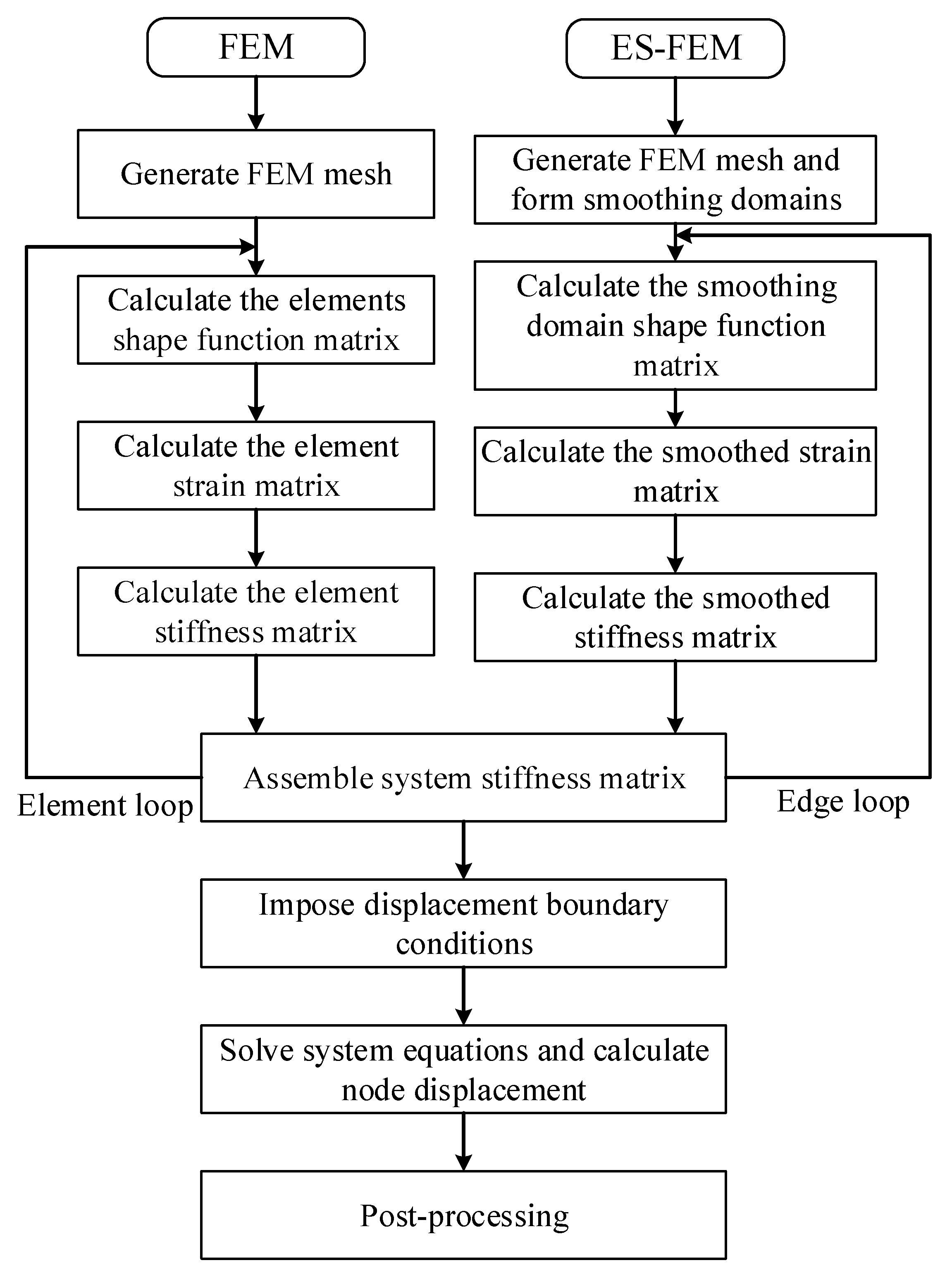
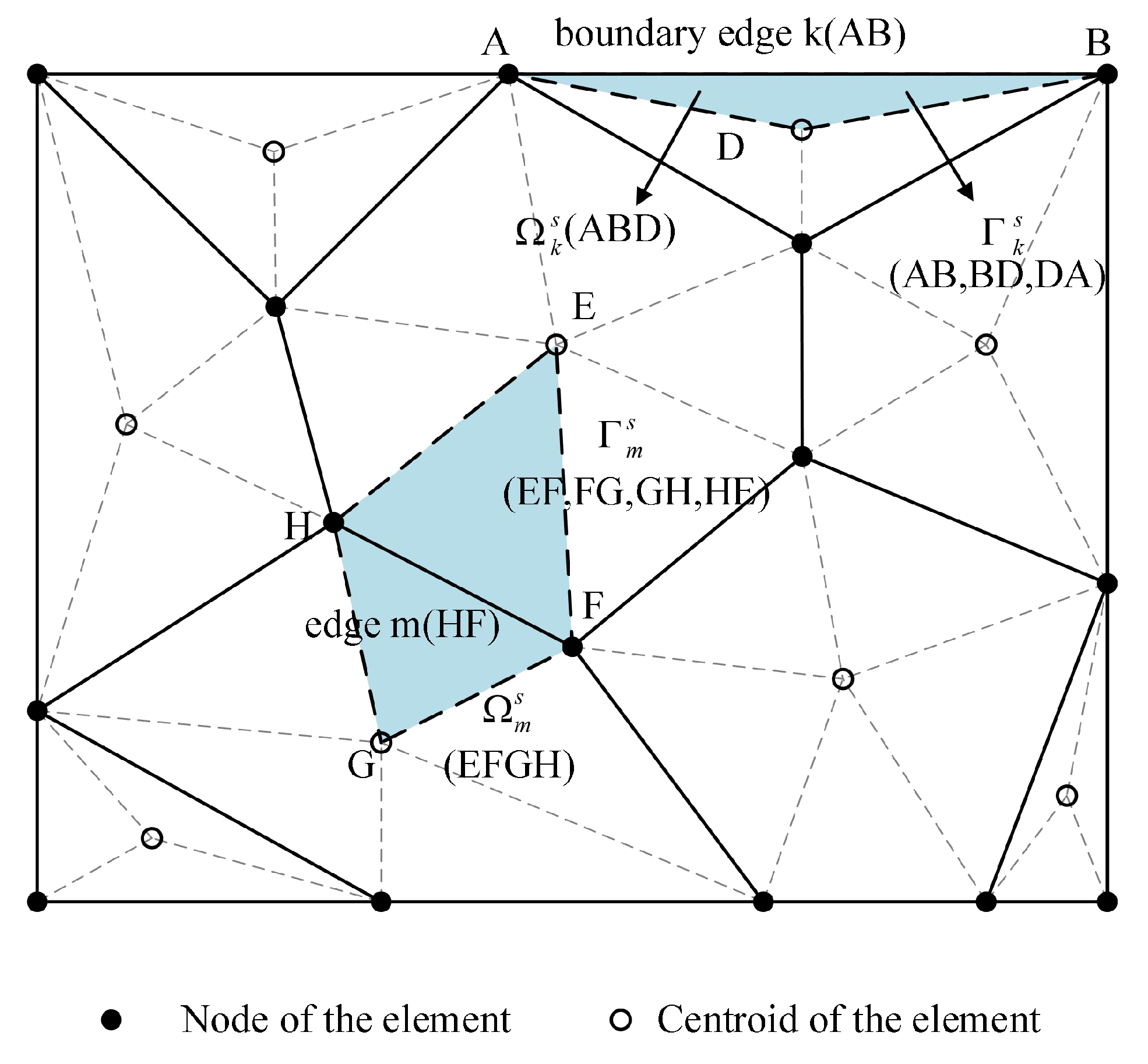
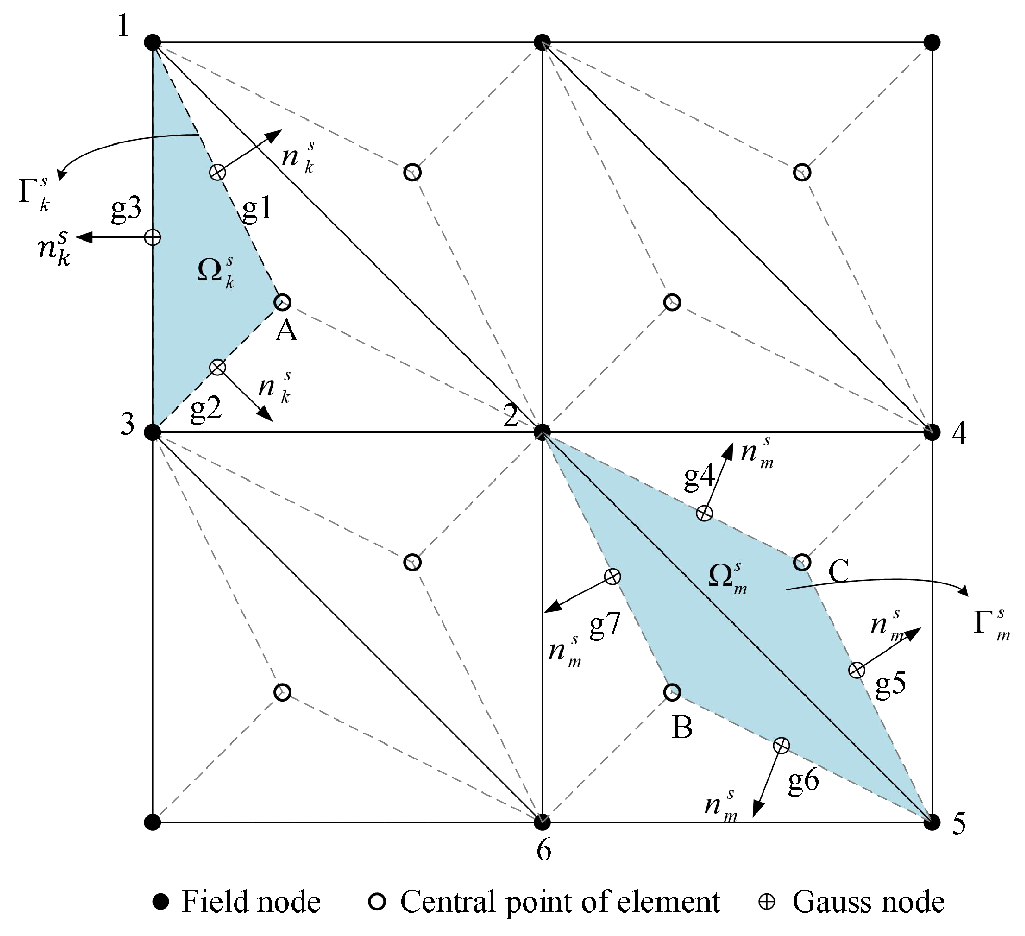
Compared with FEM, the calculation of the S-FEM has the following two differences. First, we need to construct the smoothing domains and modify or reconstruct the strain field in the S-FEM. Moreover, because the smoothing domain may involve a portion of adjacent elements, the memory requirements for S-FEM will be larger [7]. The two differences mentioned above may lead to a higher computational cost for the S-FEM than the FEM for the same grid structure. However, given the calculation cost, the results calculated by the S-FEM model are more accurate than the FEM, and thus, achieve higher efficiency. To make S-FEM more applicable to large-scale engineering problems, parallel strategies of multicore CPUs and/or multicore GPUs are usually used to improve and optimize the computational power of S-FEM.
Currently, there are many software packages developed for utilizing FEM to solve various scientific and engineering problems, while the development of software and library packages for the S-FEM is still in progress [30]. Current S-FEM software packages are mostly implemented in C++ and Fortran. However, static languages such as Fortran and C/C++ have more complex language structures, are more difficult to learn, and require high programming skills. Although high-level dynamic languages, such as MATLAB and Python, are easy to learn, highly visual and interactive, the computing speed of dynamic language is slow and there are expensive licensing fees associated with the use of commercial software such as MATLAB. Julia is an efficient, user-friendly, open-source programming language, developed by MIT in 2009 [31]. Furthermore, it balances the problems of computing performance, programming difficulty and code legibility [32].
Many researchers have used the Julia language to develop software packages related to numerical computation. For example, Frondelius et al. [33] designed an FEM structure by using the Julia language, which enables large-scale FEM models to be processed by using distributed simple programming models across a cluster of computers. Sinaie et al. [34] implemented the Material Point Method (MPM) in the Julia language. In the large strain solid mechanics simulation, only Julia’s built-in characteristics are used, which has better performance than the MPM code based on MATLAB. Zenan Huo et al. [35] implemented a package of S-FEM for linear elastic static problems by using Julia language. Pawar et al. [36] developed a one-dimensional solver for the Euler equation, and an arakawa spectral solver and pseudo-spectral solver for the two-dimensional incompressible Navier–Stokes equation for the analysis of computational fluid dynamics using the Julia language. Heitzinger et al. [37] used the Julia language to implement numerical stochastic homogeneity of elliptic problems and discussed the advantages of using Julia to solve multiscale problems involving partial differential equations. Kemmer et al. [38] designed a finite element and boundary element solver using Julia to calculate the electrostatic potential of proteins in structural solvents. Fairbrother et al. [39] developed a package for Gaussian processes, GaussianProcesses.jl, using the Julia language. GaussianProcesses.jl takes advantage of the inherent computational benefits of the Julia language, including multiple assignments and just-in-time compilation, to generate fast, flexible and user-friendly packages for Gaussian processes.
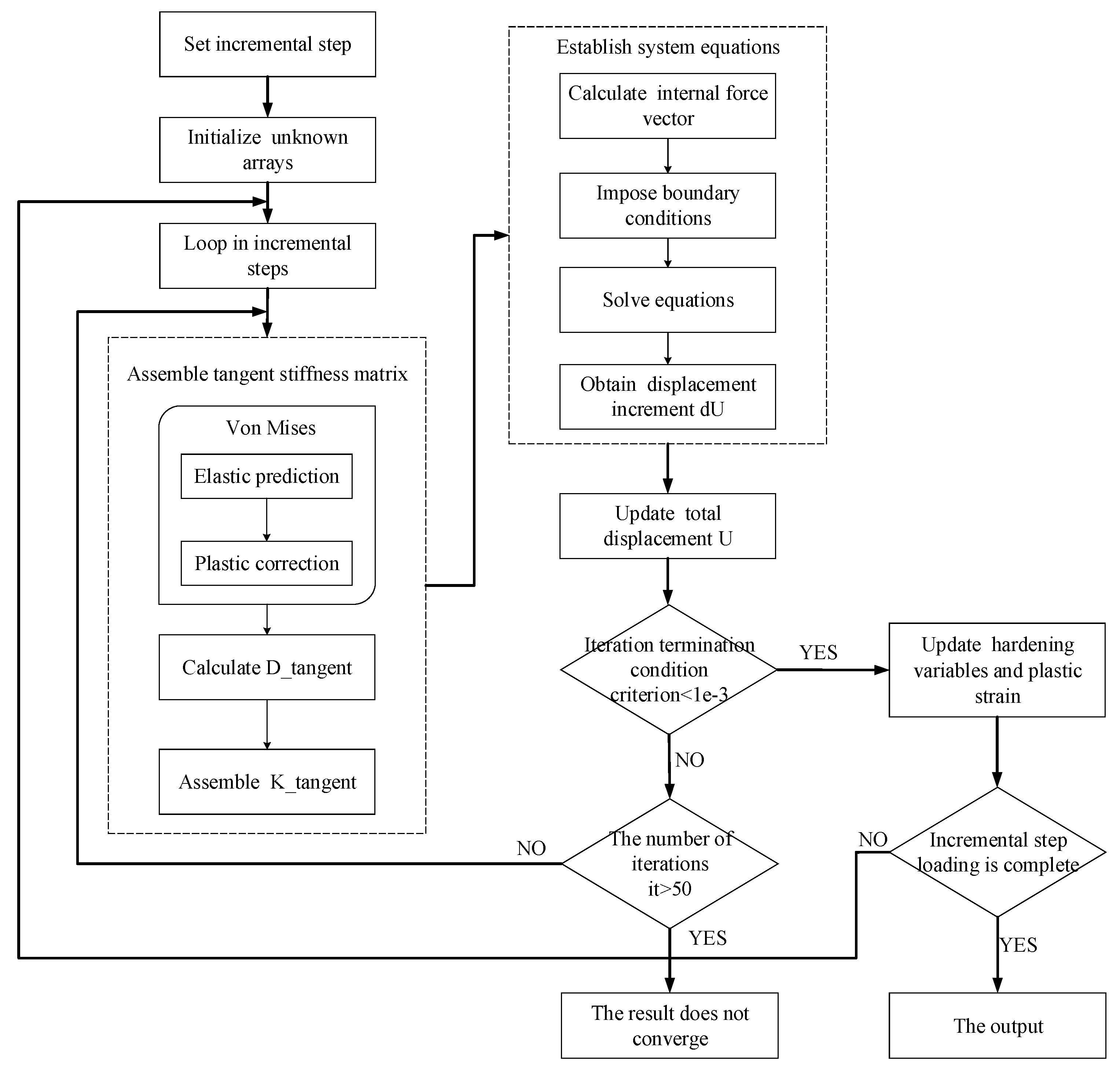
In this paper, a parallel incremental S-FEM software package epSFEM for elastic-plastic problems is designed and implemented by utilizing the Julia language on a multi-core CPU. Distributed parallelism and partitioned parallelism are used for the assembly of the stiffness matrix, allowing multiple cells to be assembled simultaneously, avoiding excessive for loops and saving computation time. The system of equations is solved using the PARDISO [40] parallel sparse matrix solver. epSFEM applies to more common and complex elastic-plastic mechanical problems in practical engineering. Moreover, epSFEM adopts an incremental theory suitable for most load cases to solve elastic-plastic problems, and the calculation results are more reliable and accurate.
The contributions of this paper can be summarized as follows:
(1) A parallel S-FEM package epSFEM using incremental theory to solve elastic-plastic problems is developed by Julia language.
(2) The computational efficiency of epSFEM is improved by using distributed and partitioned parallel strategy on a multi-core CPU.
(3) epSFEM features a clear structure and legible code and can be easily extended.
The rest of this paper is organized as follows. The theory related to S-FEM and Julia language are presented in Section 2. The detailed implementation steps of the software package epSFEM are described in Section 3. Two sets of numerical examples are used to assess the correctness of the epSFEM and to evaluate its efficiency in Section 4. The performance, strengths and weaknesses of the epSFEM and the future direction of work are discussed in Section 5. Section 6 presents the main conclusions.

2. Background

In this section, the theoretical basis of the S-FEM and parallelization strategy of the Julia language on a multicore CPU are introduced.

2.1. Smoothed Finite Element Method (S-FEM)

2.1.1. Overview of the S-FEM

The S-FEM is the implementation of the FEM by employing the strain smoothing technique to modify or reconstruct the strain field such that more accurate or special performance solutions can be obtained. NS-FEM, for example, has an upper bound solution to the model because of its weak super-convergence, insensitivity to mesh deformation and an overly soft system stiffness matrix. In the ES-FEM and FS-FEM models, there are no unphysical modes, so both methods give good results for dynamic and static problems. In the S-FEM, the most important goal is the modification of the compatible strain field or reconstruction of the strain field only from the displacement field [11]. To guarantee the stable and convergent properties of the established S-FEM model, this strain modification or reconstruction needs to be conducted in an appropriate way to obtain special characteristics. Strain modification or reconstruction can be implemented within the element, but it is generally conducted across the element to obtain more information from adjacent elements. Different modification or reconstruction methods correspond to separate S-FEMs, that is, CS-FEM, NS-FEM, ES-FEM and FS-FEM.
For two-dimensional static problems, ultra accurate numerical solutions can be obtained using ES-FEM, and the calculation results of ES-FEM based on T3 elements are even more accurate than traditional FEM with Q4 elements (same number of nodes) [11,14]. Therefore, the ES-FEM is employed to solve the two-dimensional elastic-plastic problem in this paper, and the implementation steps are introduced as follows.

2.1.2. Workflow of the ES-FEM

The ES-FEM calculation process is similar to that of the FEM, except that the ES-FEM needs to construct a smoothing domain on the basis of the FEM model and modify or reconstruct the strain field. As shown in Figure 1, many techniques designed for FEM can be adapted for ES-FEM. In short, the difference between the ES-FEM and FEM is that all calculations of the FEM are based on elements, while all calculations of the ES-FEM are conducted on smoothing domains.
The two-dimensional solid mechanics problem with problem domain Ω and boundary Γ = Γu ∪ Γt are considered, where Γu is the essential boundary where displacement conditions are prescribed and Γt is the natural or force boundary.
The calculation procedure of ES-FEM is as follows [7,11,14]:
(1) Discretization of the problem domains and construction of the smoothing domains
In the ES-FEM, general polygonal elements are used to divide the problem domain, mainly T3 elements suitable for solving two-dimensional problems. When the T3 element is used, the meshing can be the same as the standard FEM, such as the widely used Delaunay triangulation method.
As shown in Figure 2, on the basis of the polygonal element mesh, the smoothing domain is constructed. The problem domain is divided into N e polygonal elements, including N e g edges. The edge-based smoothing domain is composed of two nodes connecting one edge and the centroid of its adjacent elements. The two nodes A and B connecting edge AB and centroid D of the triangle element form the smoothing domain (ABD), see Figure 2. The construction of the smoothing domain, such as the discrete problem domain, must follow the principle of no gap and no overlap, that is, Ω = Ω 1 s Ω 2 s Ω N e s , Ω i s Ω j s = , and i j .
(2) Creation of the displacement field
The generalized displacement field u ˜ at any point in the triangular element is approximated as:
u ˜ = i = 1 N n N i ( x ) d ˜ i
where N n is the number of smoothing domain nodes, d ˜ i is the nodal displacement at node i, and N i ( x ) is the shape function:
N i ( x ) = N i ( x ) N i ( x ) n × n
where n is the degree of freedom of the smoothing domain nodes.
The Gauss integration point interpolation distribution of the ES-FEM shape function is illustrated in Figure 3. As shown in Figure 3, the commonly used linear triangular elements are employed to divide the mesh. Here, the shape function values at the Gauss integral point are calculated in two cases: boundary edge and internal edge. The results are shown in Table 1 and Table 2.
(3) Construction of the smoothed strain field
For triangular, quadrilateral and polygonal elements, strain smoothing techniques can be used to construct the strain field directly from the boundary integrals of the shape function without the need for coordinate mapping.
In the ES-FEM, the smoothed strain ε ¯ is computed as follows:
ε ¯ = Ω k s ε ˜ ( x ) Φ ( x ) d Ω
where ε ˜ ( x ) = L d u is the strain that satisfies the compatibility condition in the traditional FEM, Φ ( x ) is the smoothing function, and Ω k s is the smoothing domain, which can be defined as follows:
Φ ( x ) = 1 A k s , x Ω k s 0 , x Ω k s
where A k s is the area of the smoothing domain.
Combining the Gaussian divergence theorem, the domain integral is transformed into the edge integral to obtain the following smoothed strain calculation equation:
ε ¯ = Ω k s ε ˜ ( x ) d Ω = Ω k s L d u ˜ ( x ) d Ω = ( 1 / A k s ) Γ k s L n ( x ) u ˜ ( x ) d Γ , x Ω k s
where L d is the partial differential matrix operator, L n is the outward unit normal vector and Γ k s is the boundary of the edge-based smoothing domain.
L n ( x ) = n x 0 0 n y n y n x
where n x and n y are the x-axis and y-axis components of the normal vector outside the unit, respectively.
Similar to the FEM, the smoothed strain field is divided into:
ε ¯ ( x ) = I N n B ¯ I ( x k ) d I
where B I is the smoothed strain matrix:
B ¯ I ( x k ) = b ¯ I x ( x k ) 0 0 b ¯ I y ( x k ) b ¯ I y ( x k ) b ¯ I x ( x k )
where b ¯ I x ( x k ) and b ¯ I y ( x k ) is defined as shown in Equation (9). The boundary integral method is used to solve the smoothed strain matrix. This method is applicable to any polygonal geometry in the smoothing domain.
b ¯ I x = ( 1 / A k s ) Γ k s n x N I ( x ) d Γ = ( 1 / A k s ) i = 1 N I n i , x N I ( x i G ) l i b ¯ I y = ( 1 / A k s ) Γ k s n y N I ( x ) d Γ = ( 1 / A k s ) i = 1 N I n i , y N I ( x i G ) l i
where N I is the number of segments of Γ k s , n i , x and n i , y are the outer normal vectors of the Ith integration segment, x i G is the midpoint of each segment of the boundary, that is, the Gauss integration point, and N I ( x i G ) is the shape function value at the Gauss integration point.
(4) Establishment system of equations
The smoothed Galerkin weak form is utilized to establish the system equation in the ES-FEM. During this process, only a simple summation calculation of the relevant parameters of the smoothing domain is required.
The linear system of equations of ES-FEM is:
K ¯ ES FEM d ¯ = f ˜
where d ¯ is the displacement vector of all nodes in the S-FEM and f ˜ is the vector of all loads. K ¯ ES FEM is the system stiffness matrix of the ES-FEM and defined as Equation (11):
K ¯ IJ ES FEM = k = 1 N e g Ω k s B ¯ I T c B ¯ J d Ω = k = 1 N e g B ¯ I T c B ¯ J A k s
where c is the matrix of elasticity coefficients.
(5) Imposition of the boundary conditions
In the ES-FEM, the application process of displacement boundary conditions is similar to that of the FEM because the shape function used in the S-FEM has the same delta property as the FEM. The main methods include the direct method, set “1”, multiple large numbers, Lagrange multiplier and penalty function. The force boundary conditions are added directly to the corresponding nodes.
(6) Postprocessing
The weighted average rule is used to obtain the equivalent nodal stress in the smoothing domain, and the shape function interpolation technique is used to obtain the continuous stress field in the problem domain. The process is similar to the FEM. Finally, the accuracy of the results is assessed in relation to the actual problem.

2.2. The Julia Language

Julia, officially released in 2012, is a flexible dynamic language for scientific and numerical computation [41]. To solve large-scale numerical computation problems, parallel computing is considered essential. There are useful built-in features in Julia that make it easier for developers to design efficient parallel code. Three of the parallel strategies, that is, coroutine, multithreaded and distributed computing, are dependent on a multicore CPU. Developers can select the appropriate parallelism method for their needs. Parallel computing on many-core GPUs can be conducted by using specific packages or utilizing the built-in function of Julia and parallel arrays [1].
In this paper, parallelism on a multicore CPU is applied to effectively improve the calculation and assembly efficiency of the global stiffness matrix. In the Julia language, distributed computing based on a multicore CPU first redistributes tasks according to the number of CPU cores of the computer and then dynamically allocates computing tasks to each process so that multiple processes can be calculated at the same time, thus improving the computing efficiency. In the parallel computing of Julia language, “SharedArray” is used to reduce memory usage and improve computational efficiency. Moreover, when a “SharedArray” is employed, multiple processes are allowed to operate on the same array in the meantime [42,43].

3. The Implementation of Package epSFEM

3.1. Overview

A parallel S-FEM package using incremental theory to solve elastic-plastic problems is developed on a multicore CPU. This package contains the following three components:
Preprocessing: The preprocessing includes mesh generation and the construction of smoothing domains based on the mesh. After the preprocessing is completed, the model details of constructing the smoothing domain can be obtained, and stored in sparate five files: nodes, elements, internal edges, external edges and the centroids of mesh elements.
Solver: The solver uses incremental S-FEM to solve the elastoplastic problems, which is the main part of the whole software package. It is mainly categorized into: (1) assembly of the elastic stiffness matrix and (2) incremental loading and semismooth Newton method iterations to solve the system of equations. The calculation procedure of the incremental loading and semismooth Newton method iterations of the solver is illustrated in Figure 4.
Postprocessing: ParaView [44] is utilized to visualize the numerical calculation results. The WriteVTK.jl package in Julia is used to write the “vtu” format file needed for ParaView visualization.

3.2. Preprocessing

3.2.1. Mesh Generation

Mesh generation is the first step of the numerical analysis, which also affects the accuracy and efficiency of the numerical analysis. Currently, there are many mature mesh generation algorithms and software. The focus of this paper is on the solver section, so a simple direct generation method is used to generate the mesh and then divide the smoothing domain on this basis. Because T3 elements have good adaptability and are most used in science and engineering practice, we choose T3 elements to divide the problem domain.

3.2.2. Construction of the Smoothing Domain

Constructing the smoothing domain based on the meshing of the problem domain is one of the key tasks of the S-FEM. According to the methods of constructing the smoothing domain and storing model information in Refs. [35,45], the smoothing domain of the mesh is constructed, and the model information after dividing the smoothing domain is output. To get the best performance out of the Julia language, the following calculations can be looped in the unit of column, and the model information is stored based on the column. In this paper, we address the mesh details by integrating the features of ES-FEM and Julia parallel computation and then utilize five matrices to save the mesh details in an appropriate way; see Figure 5.
The “Node” matrix stores the x and y coordinates of the mesh nodes. The “Centroid” matrix stores the x and y coordinates of the center of the cell. The node numbers corresponding to the mesh cells are stored in the “Element”. The three node numbers of the triangular cells are stored in the three rows of “Element” in a counterclockwise order, and the number of columns is the number of mesh cells.
In the ES-FEM, the smoothing domain is constructed by using edges as the basis. We divide all the edges of the model into two categories: the outer edges are saved in the “Edge_out” matrix, and the inner edges are saved in the “Edge_in” matrix. For the matrix “Edge_out”, the two node numbers of the outer edge are stored in the first two rows, the serial number of the triangle is appended to the third row, and the rest point of the triangle is appended to the fourth row. Because one inner edge belongs to two triangles, the first two rows store the node numbers of the inner edges, the third and fourth rows of “Edge_in” are the serial numbers of neighboring triangles and the last two rows are the numbers of the other points in the triangle.

3.3. Solver

The incremental S-FEM is utilized to address the elastoplastic problem, choosing the implicit constitutive integration algorithm of the linear kinematic hardening Von Mises constitutive model and the corresponding consistent tangent modulus. First, the elastic predicted stress is calculated according to the strain of the equilibrium iteration, and then the modified stress is calculated according to a certain direction to make the stress return to the updated yield surface [46,47]. The nonlinear equations are solved by employing the semismooth Newton method.
The solution process is composed of two major procedures: (1) assembly of the elastic stiffness matrix and (2) incremental loading and semismooth Newton method iterations. The second procedure is composed of multiple incremental step cyclic calculations. Each incremental step can be divided into three steps: (1) assembly of tangent stiffness matrix, (2) solving of equations and (3) updating of hardening variables and plastic strain. According to the characteristics of parallel computing, the calculation of the latter step cannot be dependent on the previous step, so when assembling the elastic stiffness matrix, the tangent stiffness matrix can be calculated in parallel to improve efficiency. Distributed computing is used in Julia to calculate the elastic stiffness matrix and the tangent stiffness matrix for multiple elements in parallel. When solving the overall nonlinear system equations, we utilize the semismooth Newton method for each iteration. For the set of equations in each iteration, a parallel sparse equation solver, PARDISO, is used [40]. The detailed procedure of the solver in epSFEM will be presented in the subsequent sections.

3.3.1. Assembly of Elastic Stiffness Matrix

After the model is preprocessed, it needs to be assembled with an elastic stiffness matrix first. In epSFEM, we calculate the stiffness matrix of the associated smoothing domain by dividing the outer edge and the inner edge, and the calculation process is basically the same. Taking the internal edge as an example:
(1) The areas of the two triangle elements that share the inner edge is attached are computed. This process is conducted by procedure “area.jl” according to Equations (12)–(16):
a = ( x 1 x 2 ) 2 + ( y 1 y 2 ) 2
b = ( x 2 x 3 ) 2 + ( y 2 y 3 ) 2
c = ( x 3 x 1 ) 2 + ( y 3 y 1 ) 2
p = ( a + b + c ) / 2
A = ( p ( p a ) ( p b ) ( p c )
where x i and y i is the coordinate of the node i.
(2) The length of each edge of the smoothing domain is calculated in Equation (17). For the smoothing domain of the inner side, there are four edges. This process is realized in the file “lp.jl”:
l p = ( x 1 x 2 ) 2 + ( y 1 y 2 ) 2
(3) The normal outward vector v 1 is calculated for each side of the smoothing domain. This is performed in “vectorin.jl”, according to Equations (18)–(20):
y = y 2 y 1
x = x 1 x 2
v 1 = y ( y 2 + x 2 ) x ( y 2 + x 2 )
(4) Assembly of the global elastic stiffness matrix and the global smoothed strain matrix. First, the stiffness matrix of the smoothing domain element is computed and then assembled according to the smooth domain nodes. Due to the large number of zero elements in the matrix, to reduce the memory occupation, the matrix is stored in a sparse form. There are three common ways to construct sparse arrays: Compressed Sparse Row (CSR), Compressed Sparse Column (CSC) and COOrdinate (COO).
First, the COO format is used to construct the global elastic stiffness matrix, since the multi-dimensional arrays in Julia are stored according to column-based sequence. Then, for the convenience of solving the subsequent system equations, we replace it with the CSC format. To construct a sparse array according to COO format, we first need to construct three one-dimensional arrays, that is, IK_elast, JK_elast and VK_elast.
IK_elast, JK_elast and VK_elast denote the row number, column number and value of each entry in the global stiffness matrix according to the order of each row. Since the sparse functions can accumulate the entries at the same position automatically, the magnitudes of IK_elast, JK_elast and VK_elast can be predetermined.
The assembly method of the global smoothed strain matrix is basically the same as the stiffness matrix, except that when it is assembled, the rows are carried out according to the elements, and the columns are carried out according to the nodes. Three one-dimensional arrays, IB, JB and VB, are constructed in advance.
For parallel computing, the six arrays of IK_elast, JK_elast, VK_elast, IB, JB and VB need to be converted to “SharedArrays” in advance, and the elastic stiffness matrix is assembled in parallel using the “@distributed” macro in Julia. Because the stiffness matrix calculation of each element has no data dependence, there will be no data interference when performing parallel computing.
The number of processes needs to be added using the function “addprocs” before all parallel computing starts. In the parallel elastic stiffness matrix assembly, we use the “@distributed” macro to automatically allocate tasks to each process according to the number of processes and the total number of tasks for parallel computing of the loop. The total number of tasks currently is equal to the total number of smoothing domains. The “@distributed” macro is executed asynchronously on the loop; it will generate independent tasks on all available processes and return immediately without waiting for the computing to complete. To wait for the computing task to complete, the “@sync” macro must be used before the call. The procedure of assembling the elastic stiffness matrix for the internal edges by distributed parallel computation is illustrated in Algorithm 1. After the global stiffness matrix and the global smoothed strain matrix are assembled, the “Sparse” function is used to convert them into the CSC format.
Algorithm 1 Parallel calculation and assembly of the elastic stiffness matrix
Input: 
Node, Centroid, Element, Edge_in, shear, bulk
Output: 
K_elast, B
1:
Set the number of CPU cores for the Julia program.
2:
Set IK_elast, JK_elast, VK_elast, IB, JB and VB to SharedArrays.
3:
@sync @distributed begin
4:
for every internal edge do
5:
   Compute the area of the interior quadrilateral.
6:
   Compute the side lengths of the interior quadrilateral.
7:
   Compute the normal unit vectors of the four sides of the interior quadrilateral.
8:
   Compute the smoothed strain matrix of an interior quadrilateral.
9:
   Compute the stiffness matrix of an interior quadrilateral.
10:
 Compute the elastic coefficient matrix.
11:
 Assemble global stiffness matrix and smoothed strain matrix.
12:
end for
13:
end
14:
K_elast = sparse (IK_elast, JK_elast, VK_elast)
15:
B = sparse (IB, JB, VB)

3.3.2. Assembly of the Tangent Stiffness Matrix

The tangent stiffness matrix of the model needs to be calculated when solving the elastic-plastic problem using incremental theory. Equation (21) is used instead of Equation (22) to calculate the global tangent stiffness matrix. Among them, elastic stiffness matrix K elast , smoothed strain matrix B and elastic matrix D elast can be obtained in advance at the stage of assembling the elastic stiffness matrix; only elastoplastic matrix D tangent depends on the plastic model, and must be partially reorganized or modified in each Newton iteration. When most portions of the model are in the elastic stage, D tangent D elast is more sparse than D tangent [48,49].
K tangent = K elast + B T ( D tangent D elast ) B
K tangent = B T D tangent B
D tangent is calculated by the constitutive integral. The implicit discrete method is used to solve the constitutive integral, that is, elastic prediction and plastic correction. For the constitutive relation, the linear kinematic hardening Von Mises model is employed.
The steps to calculate the tangent stiffness matrix are as follows:
(1) Calculation of the smoothed strain field. Since the global smoothed strain matrix B has been calculated and assembled in the stage of assembling the elastic stiffness matrix, the smoothed strain field ε can be acquired according to the strain coordination Equation ε = Bu .
(2) The implicit Von Mises constitutive integral algorithm is used to obtain the stress S and tangent operator DS of the model, by procedure “constitutive_problem1.jl”. The formula, according to [48,49,50,51], is:
T k ( ε k ) = σ k t r , s k t r Y , σ k t r 2 G 2 G + a ( s k t r Y ) n k t r , s k t r > Y
where T k ( ε k ) represents the stress–strain operator, σ k t r = C ( ε k ε k 1 p ) , s k t r = I D σ k t r β k 1 , n k t r = s k t r s k t r , a is the hardening parameters and Y is the yield stress.
T k 0 ( ε k ) = C , s k t r Y , C 4 G 2 2 G + a I D + 4 G 2 2 G + a Y s k t r ( I D n k t r n k t r ) , s k t r > Y
where T k 0 ( ε k ) is the derivative of the stress–strain operator, C = K I I + 2 G I D , I I is the unit second-order tensor, I D = I I I 3 , K = E / 3 ( 1 2 μ ) is the bulk modulus and G = E / 2 ( 1 + μ ) is the shear modulus.
The modification of hardening variable β k and plastic strain ε k p is:
β k = β k 1 , s k t r Y , β k 1 + a 2 G + a ( s k t r Y ) n k t r , s k t r > Y
ε k p = ε k 1 p , s k t r Y , ε k 1 p + 1 2 G + a ( s k t r Y ) n k t r , s k t r > Y
where β k 1 hardening tensor from the previous incremental step and ε k 1 p plastic strain tensor from the previous incremental step.
To check whether plastic correction is needed, the array CRIT of 1 × s _ n _ e is defined representing the yield criterion, that is, s k t r Y , and the corresponding logical array IND_p of 1 × s _ n _ e with the smoothing domain of plastic behavior, where s _ n _ e represents the total number of smoothing domains. The parallel implementation of the implicit Von Mises constitutive integral is shown in Algorithm 2.
In the parallel computing of constitutive integrals, all processes can access the underlying data. To avoid conflicts, we first construct a “myrange” function to assign tasks to each process according to the number of CPU cores added. Then, the main computing process is defined as a kernel function “assembly_tangent”, and a wrapper “shared_constructive” is defined to encapsulate the kernel function. Finally, the function “constitutive_problem” is constructed to call the packaged kernel function for partition parallel computing. The “constitutive_problem” function minimizes the communication between the processes so that each process can continue to compute the allocated part for a period of time, and improve the efficiency of parallelism. The “@async” macro is used to wrap arbitrary expressions into tasks. For any content within its scope, Julia will start to run this task and then continue to execute the next code in the script without waiting for the current task to complete before executing it. The “@sync” macro means that the next task will not be executed until the dynamic closure defined by the macro “@async” is completed.
(3) Calculation of the global tangent stiffness matrix. First, the sparse elastoplastic matrix D tangent is constructed according to the tangent operator DS obtained by the constitutive integral and then the global tangent stiffness matrix is calculated according to Equation (21).
Algorithm 2 Parallel implementation of implicit Von Mises constitutive integral algorithm
Input: 
E, Ep_prev, Hard_prev, shear, bulk, a, Y, S, DS, IND_p
Output: 
S, DS, IND_p
1:
Set the number of CPU cores for the Julia program.
2:
Set E, Ep_prev, Hard_prev, S, DS, IND_p to ShareArray.
3:
Assign the number of tasks for each process according to the number of processes.
4:
for number of tasks in each process do
5:
   Check whether the smoothing domain yields according to the yield criterion.
6:
   Elastic prediction of stress tensor.
7:
   Calculate the consistent tangent operator.
8:
   Plastic correction of the stress tensor.
9:
   Plastic correction of the consistent tangent operator.
10:
end for
11:
Parallel computing using “remotecall” in Julia language.

3.3.3. Solution of System of Equations

In this process, the internal force of the model is calculated by using the stress obtained from the constitutive relationship and the smoothed strain matrix. Then, the displacement boundary conditions are applied by the direct method; that is, the corresponding rows and columns with displacement boundary conditions of “0” are deleted. A logical array Q is designed, which sets the displacement boundary condition of “0” to “0” and the rest to “1”. Then, the stiffness matrix, displacement and force are calculated with a logical array index. After that, the Pardiso.jl package is added and the “MKLPardisoSolver” solver in the package is used to solve the system of equations. Finally, the node displacement increment “ dU ” of one Newton iteration in an incremental step can be obtained.
In this paper, the semismooth Newton method is employed to solve nonlinear system of equations and check whether iteration is convergent according to Algorithm 3. “MKLPardisoSolver” is the solver in the Pardiso.jl package, Q is the logical array corresponding to the displacement boundary conditions, f is the external force vector, F is the internal force vector, the subscript k represents the kth incremental step and the superscript i t represents the i t -th iteration step, and U e 2 = U T K elast U . In each Newton iteration, the tangent stiffness matrix K tangent is used to solve the linear problem, which corresponds to the system of linear equations:
K k i t d U i t = f k F k
Algorithm 3 Newton iteration terminates judgment
1:
initialization U k 0 = U k
2:
for i t = 1 , 2 , 3 do
3:
    p s = M K L P a r d i s o S o l v e r ( )
4:
    d U i t [ Q ] = s o l v e ( p s , K k i t [ Q 1 , Q 1 ] , ( f k F k i t ) )
5:
    U k i t = U k i t 1 + d U i t
6:
    d U i t e / ( U k i t 1 e + U k i t e ) c r i t e r i o n
7:
end for
8:
set U k = U k i t

3.3.4. Update of Hardening Variable and Plastic Strain

After each incremental step is calculated, the hardening variable and plastic strain need to be updated by using Equations (25) and (26). Based on the implicit constitutive integration algorithm of Algorithm 2, the modification of the hardening variable and plastic strain is added. The parallel strategy in this part is consistent with Algorithm 2.

3.4. Postprocessing

After the execution of the solver, the widely used visualization software ParaView is used to visualize the numerical computational results. The relevant package WriteVTK.jl in Julia can write VTK XML files and use ParaView to visualize multidimensional datasets [44]. The VTK format files support include straight line (.vtr), structured mesh (.vts), image data (.vti), unstructured mesh (.vtu) and polygon data (.vtp) [52].
An unstructured mesh “vtu” format file is designed. Its implementation steps are as follows: (1) we need to define a cell type, which is defined in this paper as “VTKCellTypes.VTK_TRIANGLE”, representing the linear triangular element; (2) the “MeshCell” function is used to define the mesh model and obtain an array containing all mesh cells; (3) to generate a “vtu” format file, we need to initialize the file with mesh nodes and element information and then add node displacement data and other information to the file; (4) we can save the file as a “vtu” format file.

4. Validation and Evaluation of epSFEM

In this section, two sets of benchmark tests are performed on a powerful computational platform to evaluate the correctness and efficiency of epSFEM. The details of the workstation computer used are shown in Table 3.

4.1. Validation of the Accuracy of epSFEM

To validate the correctness of epSFEM, we use the model shown in Figure 6a to perform elastoplastic analysis and compare its calculation accuracy with traditional finite element software. In this example, a symmetric displacement boundary condition is set up on the left and bottom of the computational model. The traction force of F t = 200 N/m acts on the top of the model along the normal direction, and the traction force is added in increments through the cyclic load shown in Figure 6b. The elastic parameters are: E = 206,900 (Young’s modulus) and μ = 0.29 (Poisson’s ratio). The parameters related to plastic materials are specified as follows: a = 1000 , Y = 450 ( 2 / 3 ) . The mesh computational model with 150 triangular elements is illustrated in Figure 7a, and the computational model after constructing the smoothing domain is shown in Figure 7b.
To demonstrate the accuracy of the calculation, the displacement calculation of the model in Figure 6a is conducted, and comparisons are made in the three following cases.
(1) epSFEM is employed to calculate the displacement of a mesh model, which includes 341 nodes and 600 triangular elements (T3 elements); see Figure 8a.
(2) According to Ref. [49], the conventional FEM is used to calculate the displacement of a mesh model, which includes 341 nodes and 600 triangular elements (T3 elements); see Figure 8b.
(3) According to Ref. [49], the conventional FEM is employed to calculate the displacement of a highly accurate mesh model that includes 231,681 nodes and 76,800 eight-node quadrilateral elements (Q8 elements).
The displacements of the top node of the model calculated by the above three methods are compared in Figure 9. As shown in Figure 9, the displacement calculated by epSFEM has higher accuracy than FEM-T3 and slightly lower accuracy than FEM-Q8. Hence, the correctness of epSFEM is proven.

4.2. Evaluation of the Efficiency of epSFEM

To better analyze the computing efficiency of epSFEM, the computational efficiency of the serial and parallel versions of the epSFEM are recorded and compared. Five mesh models were created based on the same size model, shown in Figure 6a. Detailed information on the mesh is shown in Table 4.
In epSFEM, the calculation procedure can be composed of two steps: (1) assembly of the elastic stiffness matrix and (2) incremental loading and semismooth Newton method iterations. In this paper, we focus on the solution of elastic-plastic problems, so the time consumption is predominantly in the second step, which is composed of multiple incremental cyclic loading steps. Each of the incremental steps can be composed of three stages: (1) assembly of tangent stiffness matrix, (2) solving of system of equations and (3) updating of hardening variables and plastic strain. Since the Pardiso.jl package is employed to solve equations in serial and parallel code, the efficiency of solving equations in serial and parallel ways are not discussed. For the assembly of the elastic stiffness matrix, its time consumption accounts for a small proportion in the whole elastic-plastic analysis, which is not discussed in this paper. The parallel method of the hardening variable and plastic strain update part is consistent with the parallel method of tangent stiffness matrix assembly. Therefore, we mainly evaluate the computing efficiency of assembling the tangent stiffness matrix in this paper.
As shown in Figure 10, the time to compute the parallelizable section of the tangent stiffness matrix in the serial and parallel versions for five different scale mesh models is compared. As shown in Figure 10, it takes only approximately 335 s to compute a mesh model, including 2.45 million elements on the parallel version, while it takes approximately 3537.6 s to compute the same model on the serial version. On the 24-core CPU, the parallel speedup can reach 10.6.
To reflect the computational efficiency of epSFEM, we also made a comparison between commercial software and epSFEM in terms of the time required to calculate the five scale models, as shown in Table 4. The total time required for the solver computing is recorded for comparison. As shown in Figure 11, for a model containing 2.45 million elements, ABAQUS requires 10,619 s to compute, while the parallel version of epSFEM needs only 5876.3 s to complete the computation. The parallel version of epSFEM is approximately 1.8 times faster than ABAQUS.
ABAQUS was also used to calculate the displacements for a mesh model with 341 nodes and 600 triangular cells and to compare the displacements obtained by ABAQUS with those obtained by epSFEM_T3 and FEM_Q8 in Section 4.1. Using the displacement solution of FEM_Q8 as the reference solution, it can be seen that the displacement calculation accuracy of epSFEM is higher than that of ABAQUS; see Figure 12. It can be seen from the above results that the calculation time of epSFEM is shorter than that of ABAQUS when calculating the same mesh model, and the calculation accuracy of epSFEM is higher than that of ABAQUS, so the calculation efficiency of epSFEM is higher than that of ABAQUS.

5. Discussion

In this section, the capability, strengths and weaknesses of the epSFEM software package, as well as the future direction of work, are discussed.

5.1. Comprehensive Evaluation of epSFEM

5.1.1. Computational Accuracy

The accuracy of the calculation is the first guarantee for whether a software package can be used. To verify the correctness of the epSFEM calculation, a numerical example is used in Section 4.1. As listed in Table 5, the total displacement results of the six nodes at the top y = 10 m of the model are selected for comparison. Taking the displacements of FEM-Q8 as the baseline and comparing the displacements of epSFEM-T3 and FEM-T3 with them, it can be shown that the displacements of epSFEM-T3 are significantly closer to the baseline. The result difference is expressed by relative error. As seen in Table 5, for the node displacement at x = 0 and y = 10 m, the error of FEM-T3 compared with FEM-Q8 is 25.24%, while the error of epSFEM-T3 compared with FEM-Q8 is only 2.96%. This is because the S-FEM is based on the smoothing domain calculation that optimizes the system stiffness matrix and enables the displacements to be closer to the reference values.

5.1.2. Computational Efficiency

In this paper, the efficiency of computation is contrasted in two aspects: parallel speedup of parallelizable code and solver computation time; see Figure 10 and Figure 11.
In this paper, we recorded the time required to compute the parallelizable portion of the tangent stiffness matrix, that is, constitutive integral algorithm, for seven different size mesh models using serial and parallel epSFEM. As shown in Table 6, the parallel speedup is 10.2 for the computing model with 38,400 elements, increases to 14.8 for the computing model with 0.6 million elements and decreases to 10.0 for the computational model with 1.2 million elements, after which the parallel speedup increases slightly with the increase of the computational model size and basically stabilizes.
The reasons why the parallel speedup shows a pattern of increasing then decreasing and finally converging as the mesh scale increases are analyzed are as follows: (1) Parallel computing includes the time to allocate tasks; the amount of computation allocated to each process cannot be exactly the same, and there is the problem of load imbalance for each process, so the parallel speedup cannot reach the ideal parallel speedup. (2) When the mesh scale is small, such as 38,400 to 614,400, the total computation time increases as the mesh scale increases, the percentage of assigned tasks in the total time decreased, and the parallel speedup increases. (3) When the mesh scale increases to 1.2 million, the performance of the code decreases due to the larger memory allocation required and the increased garbage collection time during the code run. In the benchmark tests of this paper, the above effects do not have a significant impact on the overall performance of epSFEM as the scale continues to increase. On the contrary, it tends to a steady state.
TimerOutputs.jl package is used to test the time consumption and memory allocation in each part of the calculation process and generate the formatted table to output [53]. As listed in Table 7, the allocation of time and memory for each part of the parallel epSFEM solver when the number of elements is 600,000. Table 7 shows that the time proportion of the elastic stiffness matrix is very small, which is only 0.07% when the number of elements is 600,000. Therefore, we focus on the time and memory consumption of each part of the incremental loading and the semismooth Newton iteration, which is the plastic section in Table 7. Figure 13 presents the time occupancy of the tangent stiffness matrix assembly, solving equations, hardening variables and plastic strain updating when calculating the model with 2.45 million elements using the serial and parallel versions of epSFEM. Because the hardening variable and plastic strain only need to be updated once for each incremental step, the time proportion is the smallest. The tangent stiffness matrix assembly and solving equations need to be calculated not only for each incremental step, but also for each iteration, so the time proportion is longer. As shown in Figure 13, the proportion of time spent solving the equations in parallel computing is considerably larger than in serial computing, accounting for approximately 80%.
In summary, epSFEM combines the features of incremental theory and the parallel strategy of the Julia language to achieve a parallel and efficient incremental S-FEM for solving the elastoplastic problem. Although epSFEM can take full advantage of multicore processors, it still requires a considerable amount of time to solve linear system equations for large sparse matrices. Moreover, due to the use of incremental theory, the calculation of the latter incremental step depends on the previous incremental step, and multiple incremental steps cannot be calculated in parallel, which also limits the computational efficiency of the code.

5.2. Comparison with Other S-FEM Programs

Compared with the S-FEM packages implemented with C++, epSFEM code is more readable and convenient for further development, and has lower requirements for programming ability. In contrast with the S-FEM packages implemented by MATLAB, epSFEM does not require the payment of licensing fees for the Julia language; additionally, the computational efficiency of the Julia language is higher than that of MATLAB. Moreover, epSFEM has a clear structure and modular implementation, and each calculation step is highly customized and has the characteristics of high efficiency and simplicity.
The epSFEM is suitable to more common and complex elastoplastic mechanical problems in practical engineering and has a wider range of applications than the elastic S-FEM package implemented using the Julia language. In contrast with the elastic-plastic S-FEM package with total strain theory realized by the Julia language, epSFEM uses incremental theory suitable for most loading situations to solve elastic-plastic problems, and the calculation results are more reliable and accurate.

5.3. Outlook and Future Work

epSFEM is an incremental ES-FEM to solve two-dimensional elastoplastic problems. The next step is to expand it to an incremental FS-FEM to solve three-dimensional elastoplastic problems. Currently, the S-FEM has been commonly utilized in material mechanics and biomechanics, but it is still less applied in the field of geotechnical mechanics [54,55]. We plan to extend epSFEM to use the Mohr-Coulomb criterion combined with the strength reduction method to analyze the deformation and failure of slopes. With the maturity of artificial intelligence technology such as machine learning and deep learning, mechanical analysis and numerical simulation methods can be well integrated with machine learning, which provides a new direction for computational mechanics [56,57,58,59]. In the future, the authors wish is to use machine learning combined with epSFEM to solve partial differential Equations (PDEs), or study parameter inversion.

6. Conclusions

In this paper, a parallel incremental S-FEM package epSFEM for elastic-plastic problems has been designed and implemented by the Julia language on a multicore CPU. epSFEM has a clear structure and legible code and can be easily developed further. epSFEM utilizes incremental S-FEM to solve elastic-plastic mechanics problems for complex load cases more common in practical engineering, and the calculation results are more accurate and reliable. A partitioned parallel strategy was designed to improve the computational efficiency of epSFEM. This strategy can avoid conflicts when accessing the underlying data in parallel computing. To demonstrate the correctness of epSFEM and assess its efficiency, two sets of benchmark tests were performed in this paper. The results indicated that (1) when calculating the same mesh model, the calculation accuracy of epSFEM is higher than that of the traditional FEM; (2) it requires only 5876.3 s to calculate an elastoplastic model, consisting of approximately 2.45 million T3 elements using the parallel epSFEM software package, while it needs 10,619 s to calculate the same model using the commercial FEM software ABAQUS; (3) on a 24-core CPU, the parallel execution of epSFEM is approximately 10 times faster than the corresponding serial version.

Author Contributions

Conceptualization, M.Z., J.Q. and G.M.; methodology, M.Z. and J.Q.; software, M.Z. and Z.H.; validation, M.Z. and G.M.; formal analysis, J.Q., Z.H. and F.G.; investigation, J.Q., Z.H. and F.G.; resources, M.Z.; data curation, M.Z.; writing—original draft preparation, M.Z. and G.M.; writing—review and editing, M.Z. and G.M.; visualization, M.Z.; supervision, J.Q. and G.M.; project administration, G.M.; funding acquisition, G.M. All authors have read and agreed to the published version of the manuscript.

Funding

This research was jointly supported by the Fundamental Research Funds for China Central Universities (Grant Numbers: 2652018091) and the National Natural Science Foundation of China (Grant Numbers: 11602235).

Institutional Review Board Statement

Not applicable.

Informed Consent Statement

Not applicable.

Data Availability Statement

Not applicable.

Acknowledgments

The authors would like to thank the editor and the reviewers for their valuable comments.

Conflicts of Interest

The authors declare no conflict of interest.

Abbreviations

COOCOOrdinate
CPUCentral Processing Unit
CSCCompressed Sparse Column
CS-FEMCell-based Smoothed Finite Element Method
CSRCompressed Sparse Row
EFGElement Free Galerkin
ES-FEMEdge-based Smoothed Finite Element Method
FEMFinite Element Method
FS-FEMFace-based Smoothed Finite Element Method
GPUGraphics Processing Unit
MLPGMeshless Local Petrov-Galerkin
MPMMaterial Point Method
NS-FEMNode-based Smoothed Finite Element Method
PDEsPartial Differential Equations
RPIMRadial Point Interpolation Method
S-FEMSmoothed Finite Element Method

References

  1. Xiao, L.; Mei, G.; Xi, N.; Piccialli, F. Julia Language in Computational Mechanics: A New Competitor. Arch. Comput. Methods Eng. 2021, 29, 1713–1726. [Google Scholar] [CrossRef]
  2. Xu, N.; Mei, G.; Qin, J.; Li, Y.; Xu, L. GeoMFree3D: A package of meshfree local Radial Point Interpolation Method (RPIM) for geomechanics. Comput. Math. Appl. 2021, 81, 113–132. [Google Scholar] [CrossRef]
  3. Vizjak, J.; Bekovic, M.; Jesenik, M.; Hamler, A. Development of a Magnetic Fluid Heating FEM Simulation Model with Coupled Steady State Magnetic and Transient Thermal Calculation. Mathematics 2021, 9, 2561. [Google Scholar] [CrossRef]
  4. Li, Y.C.; Dang, S.N.; Li, W.; Chai, Y.B. Free and Forced Vibration Analysis of Two-Dimensional Linear Elastic Solids Using the Finite Element Methods Enriched by Interpolation Cover Functions. Mathematics 2022, 10, 456. [Google Scholar] [CrossRef]
  5. Liu, G.R. Meshfree Methods: Moving Beyond the Finite Element Method, 2nd ed.; CRC Press: Boca Raton, FL, USA, 2009. [Google Scholar]
  6. Liu, G.R. An Overview on Meshfree Methods: For Computational Solid Mechanics. Int. J. Comput. Methods 2016, 13, 1630001. [Google Scholar] [CrossRef]
  7. Zeng, W.; Liu, G.R. Smoothed Finite Element Methods (S-FEM): An Overview and Recent Developments. Arch. Comput. Methods Eng. 2018, 25, 397–435. [Google Scholar] [CrossRef]
  8. Liu, G.R.; Zhang, G.Y. Smoothed Point Interpolation Methods: G Space Theory and Weakened Weak Forms; World Scientific: Singapore, 2013. [Google Scholar]
  9. Ding, R.; Shen, Q.; Yao, Y. The element-free Galerkin method for the dynamic Signorini contact problems with friction in elastic materials. Appl. Math. Comput. 2022, 415, 126696. [Google Scholar] [CrossRef]
  10. Liu, Z.; Wei, G.; Qin, S.; Wang, Z. The elastoplastic analysis of functionally graded materials using a meshfree RRKPM. Appl. Math. Comput. 2022, 413, 126651. [Google Scholar] [CrossRef]
  11. Liu, G.R.; Trung, N.T. Smoothed Finite Element Methods; CRC Press: Boca Raton, FL, USA, 2016. [Google Scholar]
  12. Cui, X.Y.; Liu, G.R.; Li, G.Y.; Zhang, G.Y.; Sun, G.Y. Analysis of elastic-plastic problems using edge-based smoothed finite element method. Int. J. Press. Vessel. Pip. 2009, 86, 711–718. [Google Scholar] [CrossRef]
  13. Cazes, F.; Meschke, G. An edge-based smoothed finite element method for 3D analysis ofsolid mechanics problems. Int. J. Numer. Methods Eng. 2013, 94, 715–739. [Google Scholar] [CrossRef]
  14. Liu, G.R.; Nguyen-Thoi, T.; Lam, K.Y. An edge-based smoothed finite element method (ES-FEM) for static, free and forced vibration analyses of solids. J. Sound Vib. 2009, 320, 1100–1130. [Google Scholar] [CrossRef]
  15. Nguyen-Thoi, T.; Phung-Van, P.; Rabczuk, T.; Nguyen-Xuan, H.; Le-Van, C. Free and forced vibration analysis using the n-sided polygonal cell-based smoothed finite element method (nCS-FEM). Int. J. Comput. Methods 2013, 10, 1340008. [Google Scholar] [CrossRef]
  16. Tian, F.; Tang, X.; Xu, T.; Li, L. An adaptive edge-based smoothed finite element method (ES-FEM) for phase-field modeling of fractures at large deformations. Comput. Methods Appl. Mech. Eng. 2020, 372, 113376. [Google Scholar] [CrossRef]
  17. Cui, X.Y.; Liu, G.R.; Li, G.Y.; Zhao, X.; Nguyen, T.T.; Sun, G.Y. A smoothed finite element method (SFEM) for linear and geometrically nonlinear analysis of plates and shells. Comput. Model. Eng. Sci. 2008, 28, 109–125. [Google Scholar]
  18. Zhang, Z.Q.; Liu, G.R.; Khoo, B.C. Immersed smoothed finite element method for two dimensional fluid–structure interaction problems. Int. J. Numer. Methods Eng. 2012, 90, 1292–1320. [Google Scholar] [CrossRef]
  19. He, Z.C.; Liu, G.R.; Zhong, Z.H.; Zhang, G.Y.; Cheng, A.G. Coupled analysis of 3D structural-acoustic problems using the edge-based smoothed finite element method/finite element method. Finite Elem. Anal. Des. 2010, 46, 1114–1121. [Google Scholar] [CrossRef]
  20. Li, E.; Zhang, Z.; He, Z.C.; Xu, X.; Liu, G.R.; Li, Q. Smoothed finite element method with exact solutions in heat transfer problems. Int. J. Heat Mass Transf. 2014, 78, 1219–1231. [Google Scholar] [CrossRef]
  21. Jiang, C.; Zhang, Z.Q.; Liu, G.R.; Han, X.; Zeng, W. An edge-based/node-based selective smoothed finite element method using tetrahedrons for cardiovascular tissues. Eng. Anal. Bound. Elem. 2015, 59, 62–77. [Google Scholar] [CrossRef]
  22. Lee, K.; Lim, J.H.; Sohn, D.; Im, S. A three-dimensional cell-based smoothed finite element method for elasto-plasticity. J. Mech. Sci. Technol. 2015, 29, 611–623. [Google Scholar] [CrossRef]
  23. Liu, G.R.; Nguyen-Thoi, T.; Nguyen-Xuan, H.; Lam, K.Y. A node-based smoothed finite element method (NS-FEM) for upper bound solutions to solid mechanics problems. Comput. Struct. 2009, 87, 14–26. [Google Scholar] [CrossRef]
  24. Li, Y.; Liu, G. A novel node-based smoothed finite element method with linear strain fields for static, free and forced vibration analyses of solids. Appl. Math. Comput. 2019, 352, 30–58. [Google Scholar] [CrossRef]
  25. Nguyen-Thoi, T.; Liu, G.R.; Lam, K.Y.; Zhang, G.Y. A face-based smoothed finite element method (FS-FEM) for 3D linear and geometrically non-linear solid mechanics problems using 4-node tetrahedral elements. Int. J. Numer. Methods Eng. 2009, 78, 324–353. [Google Scholar] [CrossRef]
  26. Chen, L.; Rabczuk, T.; Bordas, S.P.A.; Liu, G.R.; Zeng, K.Y.; Kerfriden, P. Extended finite element method with edge-based strain smoothing (ESm-XFEM) for linear elastic crack growth. Comput. Methods Appl. Mech. Eng. 2012, 209, 250–265. [Google Scholar] [CrossRef]
  27. Nguyen-Xuan, H.; Liu, G.R. An edge-based smoothed finite element method softened with a bubble function (bES-FEM) for solid mechanics problems. Comput. Struct. 2013, 128, 14–30. [Google Scholar] [CrossRef]
  28. Xu, X.; Gu, Y.; Liu, G. A Hybrid smoothed finite element method (H-SFEM) to solid mechanics problems. Int. J. Comput. Methods 2013, 10, 1340011. [Google Scholar] [CrossRef]
  29. Zeng, W.; Liu, G.R.; Li, D.; Dong, X.W. A smoothing technique based beta finite element method (beta FEM) for crystal plasticity modeling. Comput. Struct. 2016, 162, 48–67. [Google Scholar] [CrossRef]
  30. Dudzinski, M.; Rozgić, M.; Stiemer, M. oFEM: An object oriented finite element package for Matlab. Appl. Math. Comput. 2018, 334, 117–140. [Google Scholar] [CrossRef]
  31. Gao, K.; Mei, G.; Piccialli, F.; Cuomo, S.; Tu, J.; Huo, Z. Julia language in machine learning: Algorithms, applications, and open issues. Comput. Sci. Rev. 2020, 37, 100254. [Google Scholar] [CrossRef]
  32. Bezanson, J.; Edelman, A.; Karpinski, S.; Shah, V.B. Julia: A Fresh Approach to Numerical Computing. SIAM Rev. 2017, 59, 65–98. [Google Scholar] [CrossRef]
  33. Frondelius, T.; Aho, J. JuliaFEM-open source solver for both industrial and academia usage. Raken. Mek. 2017, 50, 229–233. [Google Scholar] [CrossRef]
  34. Sinaie, S.; Nguyen, V.P.; Nguyen, C.T.; Bordas, S. Programming the material point method in Julia. Adv. Eng. Softw. 2017, 105, 17–29. [Google Scholar] [CrossRef]
  35. Huo, Z.; Mei, G.; Xu, N. juSFEM: A Julia-based open-source package of parallel Smoothed Finite Element Method (S-FEM) for elastic problems. Comput. Math. Appl. 2021, 81, 459–477. [Google Scholar] [CrossRef]
  36. Pawar, S.; San, O. CFD Julia: A Learning Module Structuring an Introductory Course on Computational Fluid Dynamics. Fluids 2019, 4, 159. [Google Scholar] [CrossRef]
  37. Heitzinger, C.; Tulzer, G. Julia and the numerical homogenization of PDEs. In Proceedings of the 1st Workshop on High Performance Technical Computing Dynamic Languages, New Orleans, LA, USA, 17 November 2014; pp. 36–40. [Google Scholar] [CrossRef]
  38. Kemmer, T.; Rjasanow, S.; Hildebrandt, A. NESSie.jl–Efficient and intuitive finite element and boundary element methods for nonlocal protein electrostatics in the Julia language. J. Comput. Sci. 2018, 28, 193–203. [Google Scholar] [CrossRef]
  39. Fairbrother, J.; Nemeth, C.; Rischard, M.; Brea, J.; Pinder, T. GaussianProcesses.jl: A Nonparametric Bayes Package for the Julia Language. J. Stat. Softw. 2022, 102, 1–36. [Google Scholar] [CrossRef]
  40. Pardiso.jl. 2021. Available online: https://github.com/JuliaSparse/Pardiso.jl (accessed on 10 February 2021).
  41. The Julia Programming Language. 2021. Available online: https://julialang.org/ (accessed on 5 January 2021).
  42. Huo, Z.; Mei, G.; Casolla, G.; Giampaolo, F. Designing an efficient parallel spectral clustering algorithm on multi-core processors in Julia. J. Parallel Distrib. Comput. 2020, 138, 211–221. [Google Scholar] [CrossRef]
  43. Julia 1.6 Documentation. 2021. Available online: https://docs.julialang.org/en/v1/ (accessed on 10 May 2021).
  44. Paraview. 2019. Available online: https://www.paraview.org/ (accessed on 28 May 2021).
  45. Li, Y.; Yue, J.H.; Niu, R.P.; Liu, G.R. Automatic mesh generation for 3D smoothed finite element method (S-FEM) based on the weaken-weak formulation. Adv. Eng. Softw. 2016, 99, 111–120. [Google Scholar] [CrossRef]
  46. Dodds, R.H., Jr. Numerical techniques for plasticity computations in finite element analysis. Comput. Struct. 1987, 26, 767–779. [Google Scholar] [CrossRef]
  47. Blaheta, R. Convergence of Newton-type methods in incremental return mapping analysis of elasto-plastic problems. Comput. Methods Appl. Mech. Eng. 1997, 147, 167–185. [Google Scholar] [CrossRef]
  48. De Souza Neto, E.A.; Peri, D.; Owen, D.R.J. Computational Methods for Plasticity; Wiley: Hoboken, NJ, USA, 2008. [Google Scholar]
  49. Čermák, M.; Sysala, S.; Valdman, J. Efficient and flexible MATLAB implementation of 2D and 3D elastoplastic problems. Appl. Math. Comput. 2019, 355, 595–614. [Google Scholar] [CrossRef]
  50. Carstensen, C.; Klose, R. Elastoviscoplastic finite element analysis in 100 lines of Matlab. J. Numer. Math. 2002, 10, 157–192. [Google Scholar] [CrossRef]
  51. Sysala, S. Properties and simplifications of constitutive time-discretized elastoplastic operators. ZAMM-J. Appl. Math. Mech./Z. für Angew. Math. Und Mech. 2014, 94, 233–255. [Google Scholar] [CrossRef]
  52. WriteVTK.jl. 2021. Available online: https://github.com/jipolanco/WriteVTK.jl (accessed on 10 June 2021).
  53. TimerOutputs.jl. 2021. Available online: https://github.com/KristofferC/TimerOutputs.jl (accessed on 10 August 2021).
  54. Ma, Z.; Mei, G. Deep learning for geological hazards analysis: Data, models, applications, and opportunities. Earth-Sci. Rev. 2021, 223, 103858. [Google Scholar] [CrossRef]
  55. Mei, G.; Xu, N.; Qin, J.; Wang, B.; Qi, P. A Survey of Internet of Things (IoT) for Geohazard Prevention: Applications, Technologies, and Challenges. IEEE Internet Things J. 2020, 7, 4371–4386. [Google Scholar] [CrossRef]
  56. Rudy, S.; Alla, A.; Brunton, S.; Kutz, J. Data-driven identification of parametric partial differential equations. SIAM J. Appl. Dyn. Syst. 2019, 18, 643–660. [Google Scholar] [CrossRef]
  57. Raissi, M.; Perdikaris, P.; Karniadakis, G. Physics-informed neural networks: A deep learning framework for solving forward and inverse problems involving nonlinear partial differential equations. J. Comput. Phys. 2019, 378, 686–707. [Google Scholar] [CrossRef]
  58. Haghighat, E.; Raissi, M.; Moure, A.; Gomez, H.; Juanes, R. A physics-informed deep learning framework for inversion and surrogate modeling in solid mechanics. Comput. Methods Appl. Mech. Eng. 2021, 379, 113741. [Google Scholar] [CrossRef]
  59. Jacobs, B.; Celik, T. Unsupervised document image binarization using a system of nonlinear partial differential equations. Appl. Math. Comput. 2022, 418, 126806. [Google Scholar] [CrossRef]
Figure 1. Flow chart of the FEM and ES-FEM.
Mathematics 10 02024 g001
Figure 2. Polygon element mesh and the edge-based smoothing domain in ES-FEM.
Mathematics 10 02024 g002
Figure 3. Illustration of the interpolation distribution of the Gaussian integration points of the ES-FEM shape function.
Mathematics 10 02024 g003
Figure 4. Illustration of the calculation procedure of incremental loading and semismooth Newton method iterations.
Mathematics 10 02024 g004
Figure 5. Illustration of the matrices “Node”, “Centroid”, “Element”, “Edge_out” and “Edge_in”, using two adjacent triangles as examples.
Mathematics 10 02024 g005
Figure 6. (a) Simplified 2D geometry of the elastic-plastic problem and (b) history of the traction force.
Mathematics 10 02024 g006
Figure 7. (a) A mesh computational model with 150 triangular elements and (b) a computational model after constructing the smoothing domain.
Mathematics 10 02024 g007
Figure 8. (a) The contour of displacement calculated using epSFEM and (b) the contour of displacement calculated using FEM-T3.
Mathematics 10 02024 g008
Figure 9. Comparison curves of node displacements at the top of the model calculated by different methods.
Mathematics 10 02024 g009
Figure 10. Comparison of serial and parallel epSFEM computing time of the parallelizable section of the tangent stiffness matrix.
Mathematics 10 02024 g010
Figure 11. Comparison of the computation time of serial and parallel epSFEM and ABAQUS solvers for elastic-plastic problems.
Mathematics 10 02024 g011
Figure 12. Comparison curves of node displacements at the top of the model calculated with ABAQUS and epsFEM.
Mathematics 10 02024 g012
Figure 13. The proportion of time in each part of the epSFEM solver when calculating the model with 2.45 million elements using (a) the serial version of epSFEM and (b) the parallel version of epSFEM.
Mathematics 10 02024 g013
Table 1. The shape function entries at different points on the boundary of the smoothing domain connected to the outer edge 1–2 in Figure 3.
Node Number123Node Attributes
11.00.00.0Field node
20.01.00.0Field node
30.00.01.0Field node
A1/31/31/3Centroid of element
g11/21/20.0Gauss point
g21/64/61/6Gauss point
g34/61/61/6Gauss point
Table 2. The shape function entries at different points on the internal smoothing domain connected with the inner edges 3–5 in Figure 3.
Node Number3456Node Attributes
31.00.00.00.0Field node
40.01.00.00.0Field node
50.00.01.00.0Field node
60.00.00.01.0Field node
B1/31/31/30.0Centroid of element
C1/30.01/31/3Centroid of element
g44/61/61/60.0Gauss point
g51/61/64/60.0Gauss point
g61/60.04/61/6Gauss point
g74/60.01/61/6Gauss point
Table 3. Specifications of the workstation computer for performing the benchmark tests.
SpecificationsDetails
CPUIntel Xeon Gold 5118 CPU
CPU Cores24
CPU Frequency2.30 GHz
CPU RAM128 GB
OSWindows 10 professional
IDEVisual studio Code
JuliaVersion 1.5.2
Table 4. Details of the used five mesh models.
Mesh Models (T3)Number of NodesNumber of Elements
1173,761345,600
2308,481614,400
3609,3011,215,000
4909,7011,815,000
51,231,3612,457,600
Table 5. Validation of the accuracy of the epSFEM by comparison of calculated displacements.
PositionMethodRelative Error
FEM-T3epSFEM-T3FEM-Q8FEM-T3epSFEM-T3
0.0 m0.02223 m0.02704 m0.02784 m25.24%2.96%
2.0 m0.02095 m0.02583 m0.02680 m27.92%3.76%
4.0 m0.01787 m0.02217 m0.02423 m35.59%9.29%
6.0 m0.01267 m0.01572 m0.01640 m29.44%4.33%
8.0 m0.00744 m0.00896 m0.00924 m24.19%3.13%
10.0 m0.00626 m0.00788 m0.00819 m30.83%3.93%
Table 6. The parallel speedup of the parallelizable section of the tangential stiffness matrix.
Number of NodesNumber of ElementsComputing Time (s)
Single-CoreMulti-Core (24-Core)Parallel Speedup
19,52138,40069.76.8310.2
77,441153,600283.323.512.05
173,761345,600772.256.513.7
308,481614,4001297.687.714.8
609,3011,215,0001728.6172.910.0
909,7011,815,0002546251.910.1
1,231,3612,457,6003537.633510.6
Table 7. Time and memory allocation of each part of the parallel epSFEM solver when the number of elements is 600,000.
Tot /% Measured TimeAllocation
1256.9 s/100%337.83 GiB/100%
SectionncallsTime%totavgalloc%totavg
solver11256.9 s100%1256.9 s337.83 GiB100%337.83 GiB
   elastic10.9 s0.07%0.9 s1.83 GiB0.54%1.83 GiB
   plastic11256 s99.93%1256 s336 GiB99.46%336 GiB
      solving132946 s75.3%7.16 s62.6 GiB18.53%486 MiB
      assembly132246 s19.6%1.86 s256 GiB75.78%1.94 GiB
         constitutive13287.7 s6.98%664 ms62.0 MiB0.02%481 KiB
         K_tangent132150.1 s11.95%1.14 s252 GiB74.6%1.91 GiB
      hardening and strain4033.0 s2.62%824 ms1.03 GiB0.3%26.3 MiB
Publisher’s Note: MDPI stays neutral with regard to jurisdictional claims in published maps and institutional affiliations.

