
A Simplified Radial Basis Function Method with Exterior Fictitious Sources for Elliptic Boundary Value Problems


Abstract
:1. Introduction
2. Methodology
2.1. Elliptic Boundary Value Problems
2.2. Simplified Radial Basis Functions
2.3. Discretization
2.3.1. Discretization in Two Dimensions
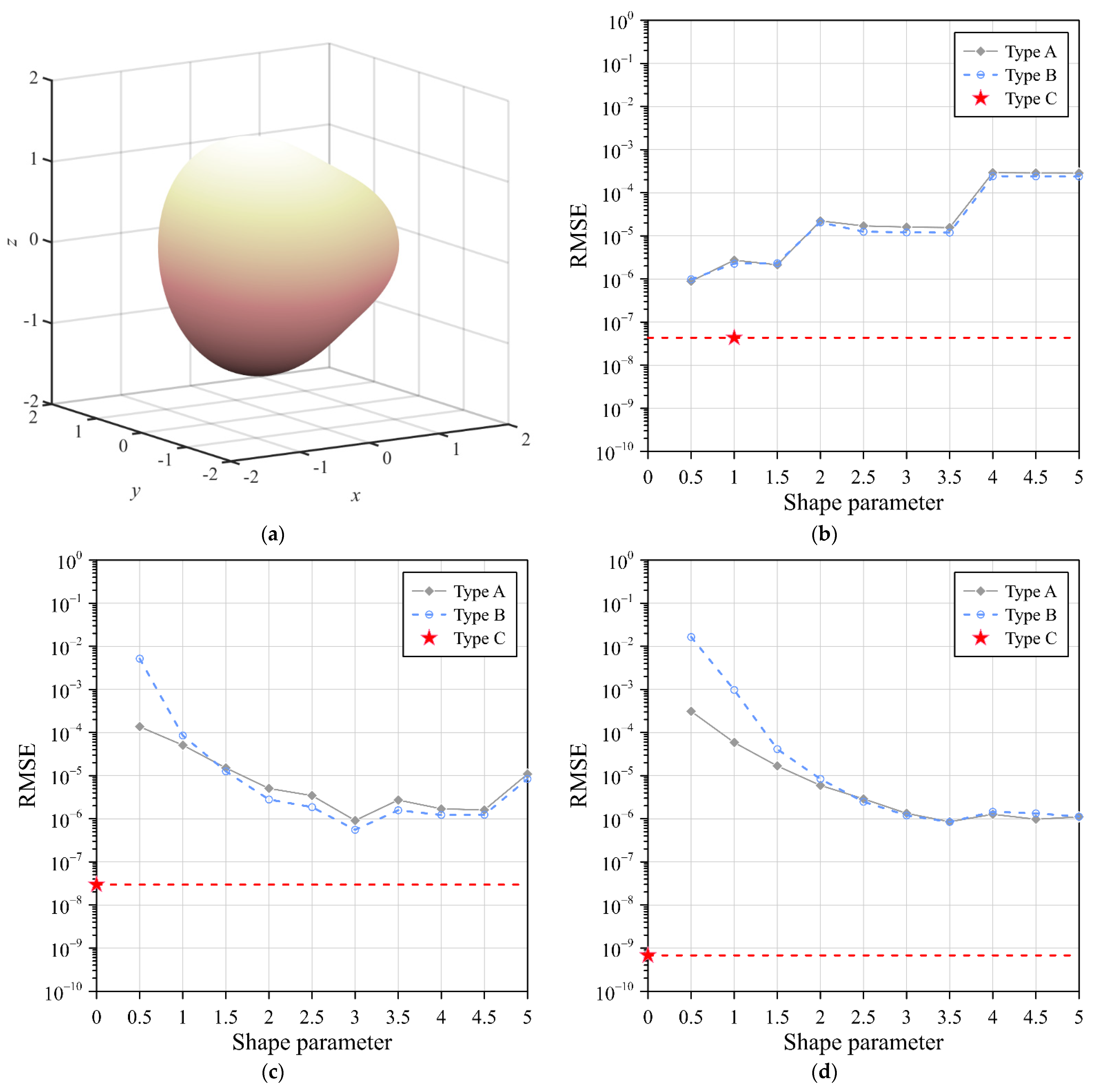
2.3.2. Discretization in Three Dimensions
2.4. Location of Fictitious Sources
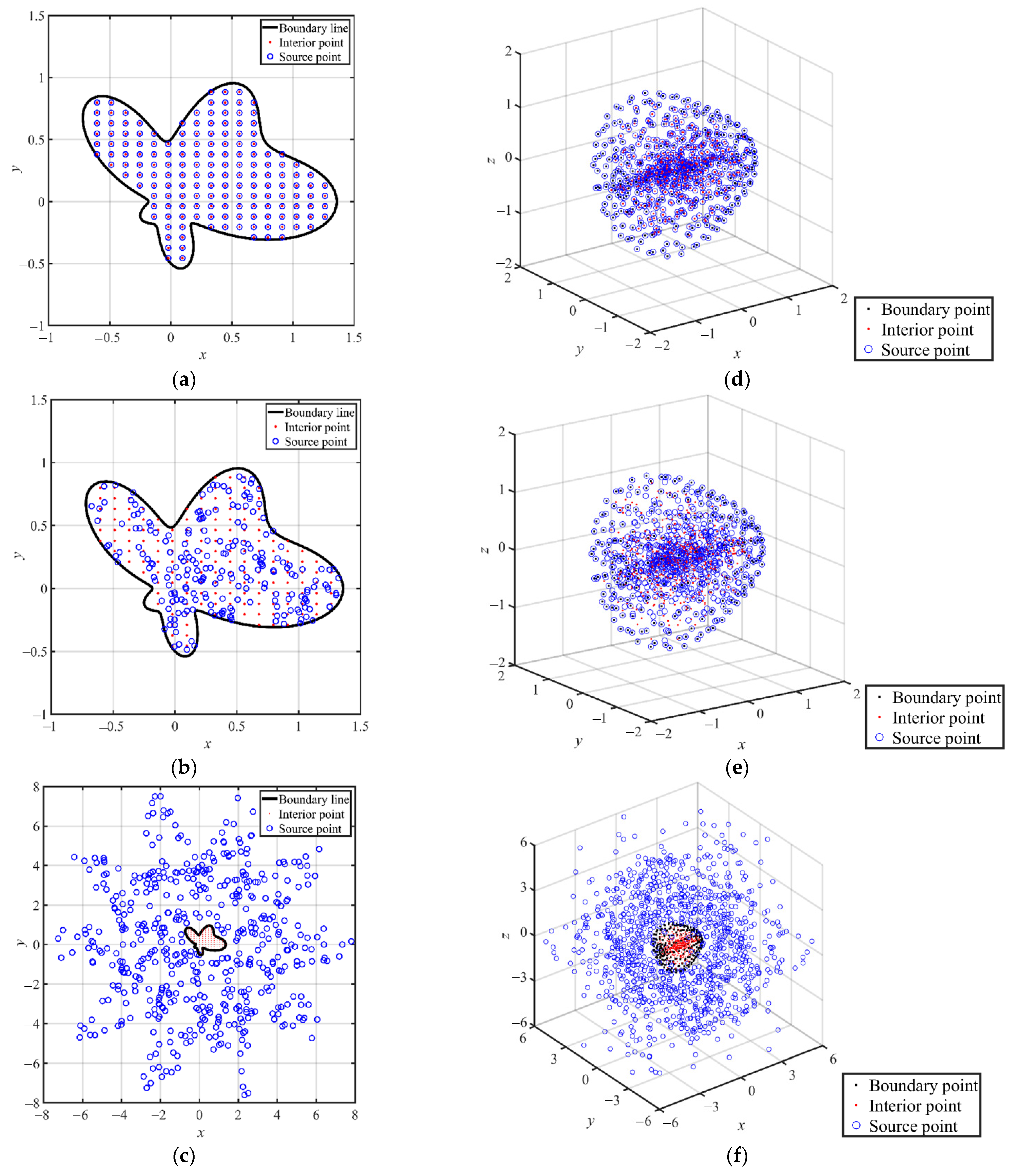
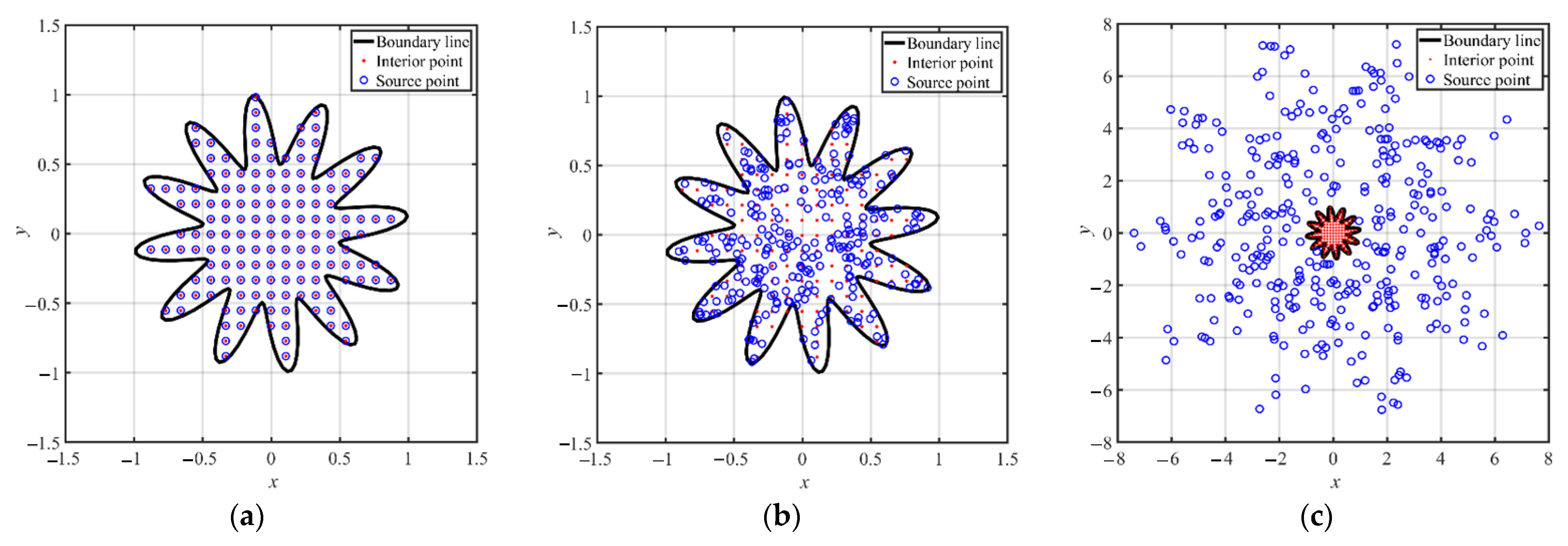
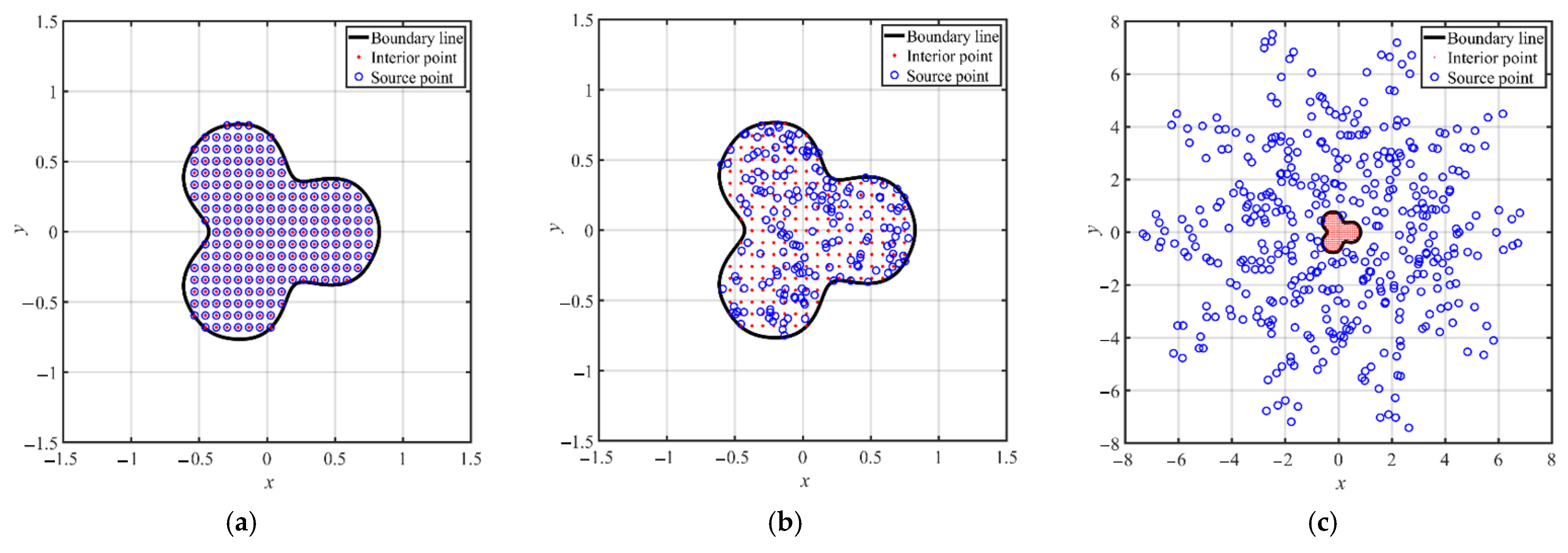
2.4.1. Type A: Uniform Centers
2.4.2. Type B: Randomly Fictitious Centers
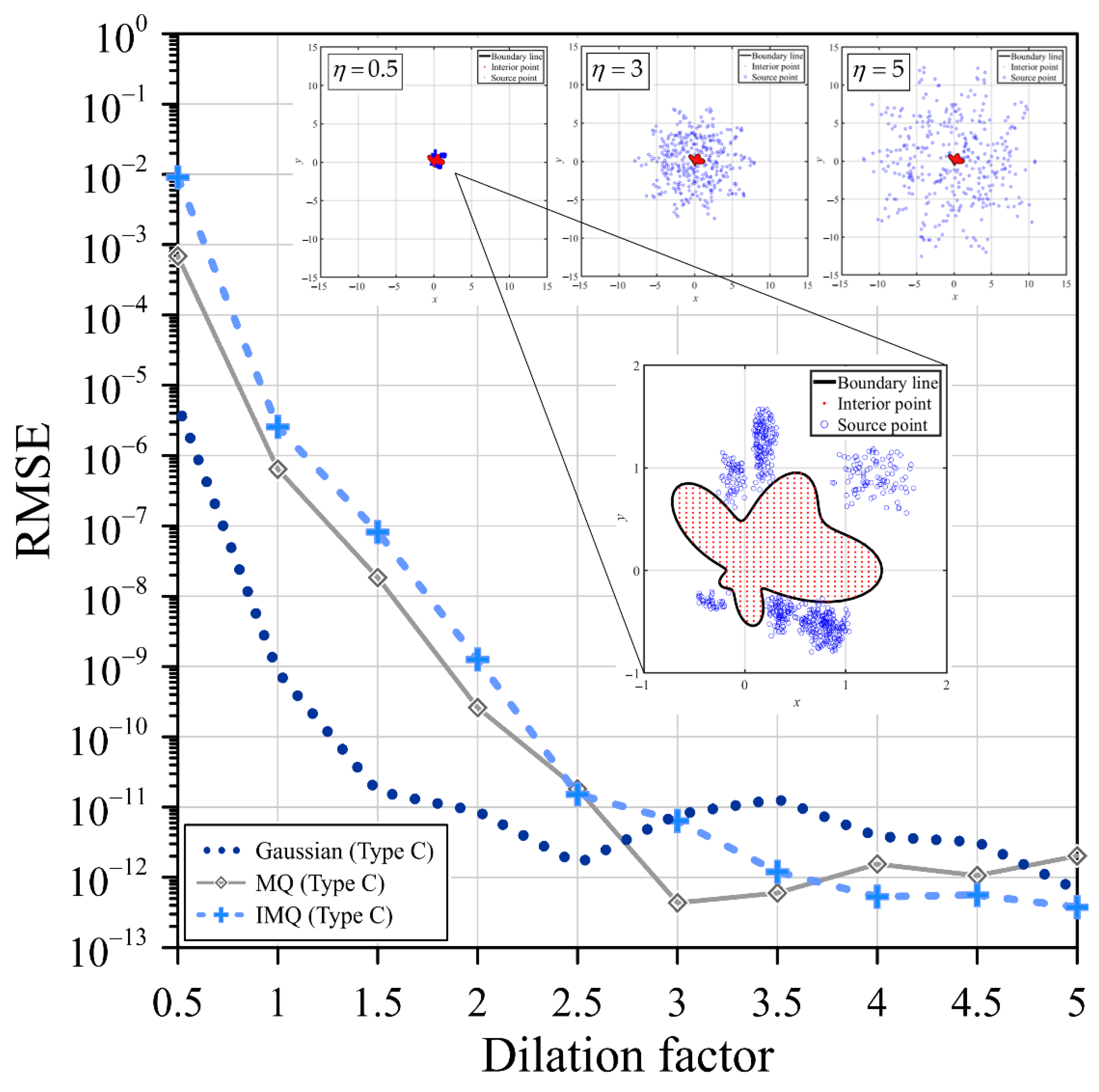
2.4.3. Type C: Exterior Fictitious Sources
3. Validation of the Methodology
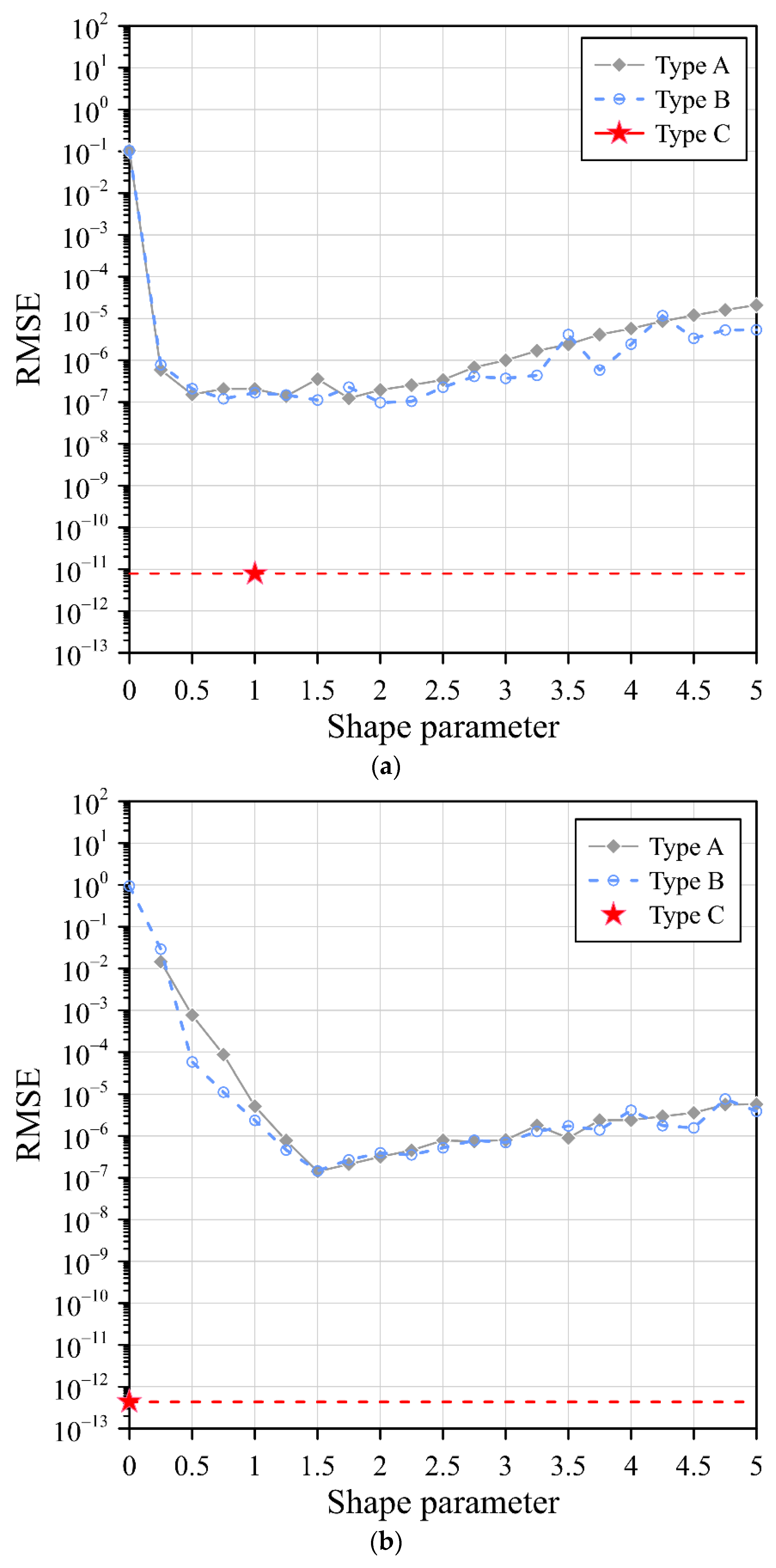
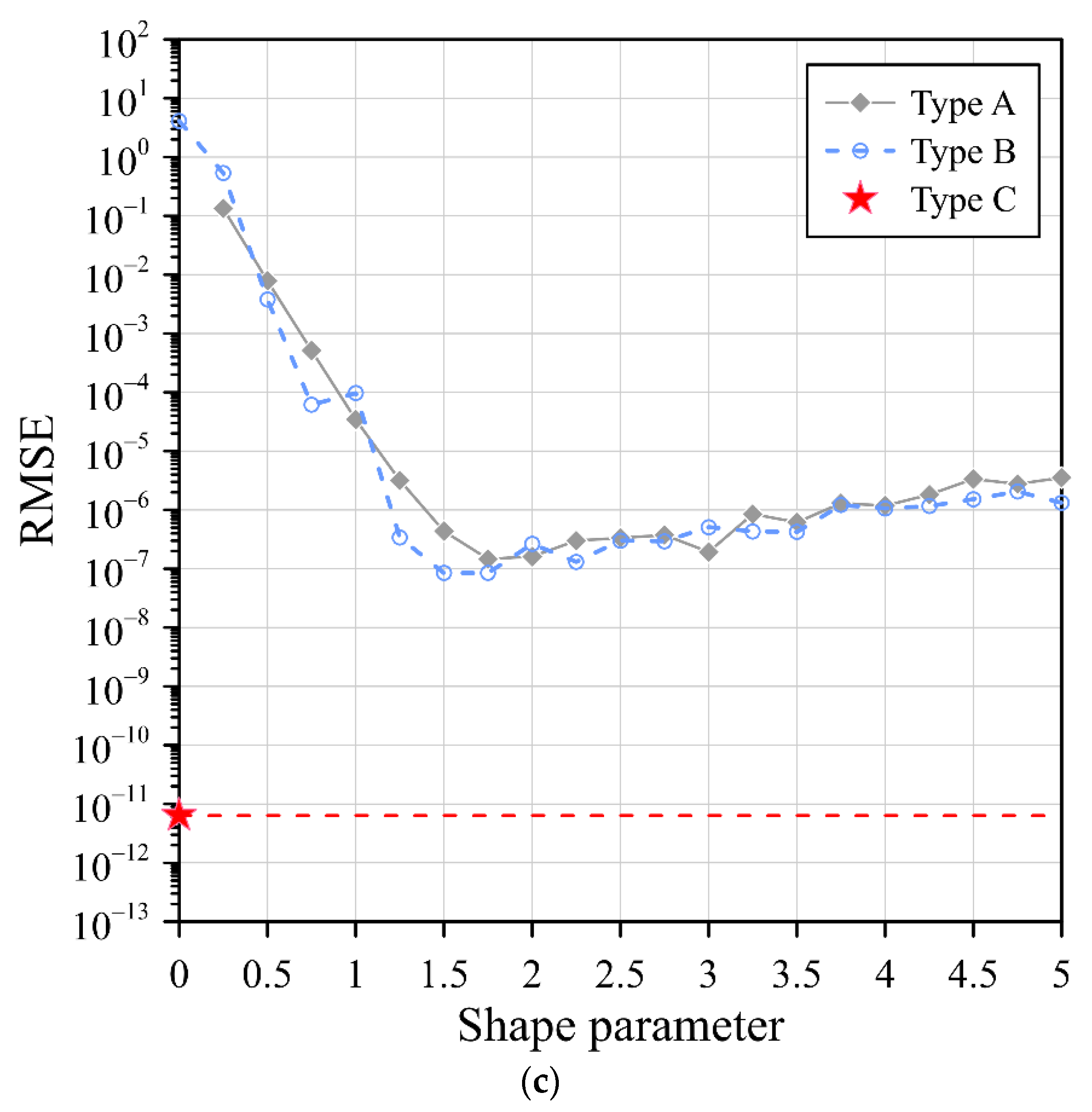
3.1. Example 1
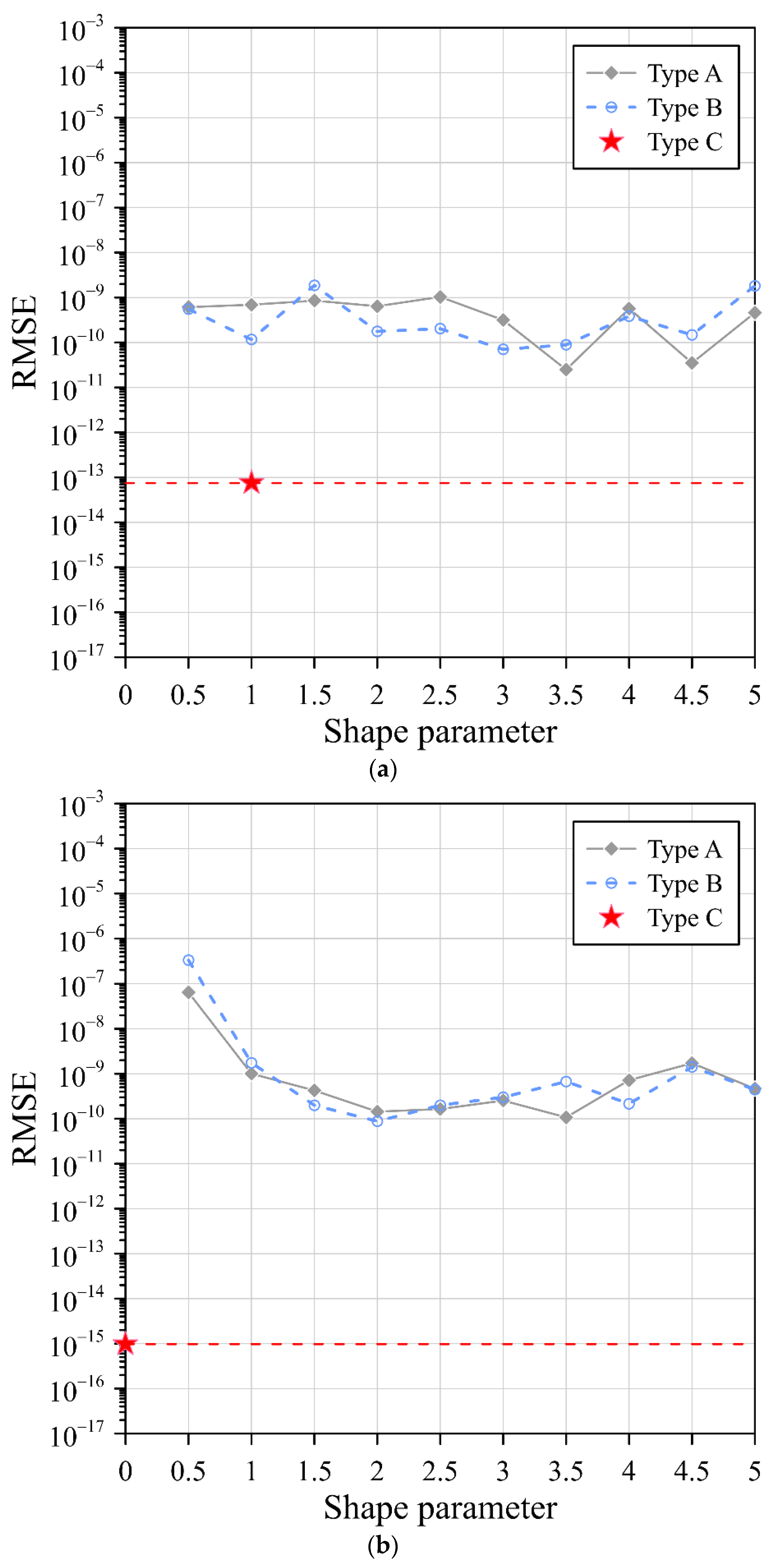
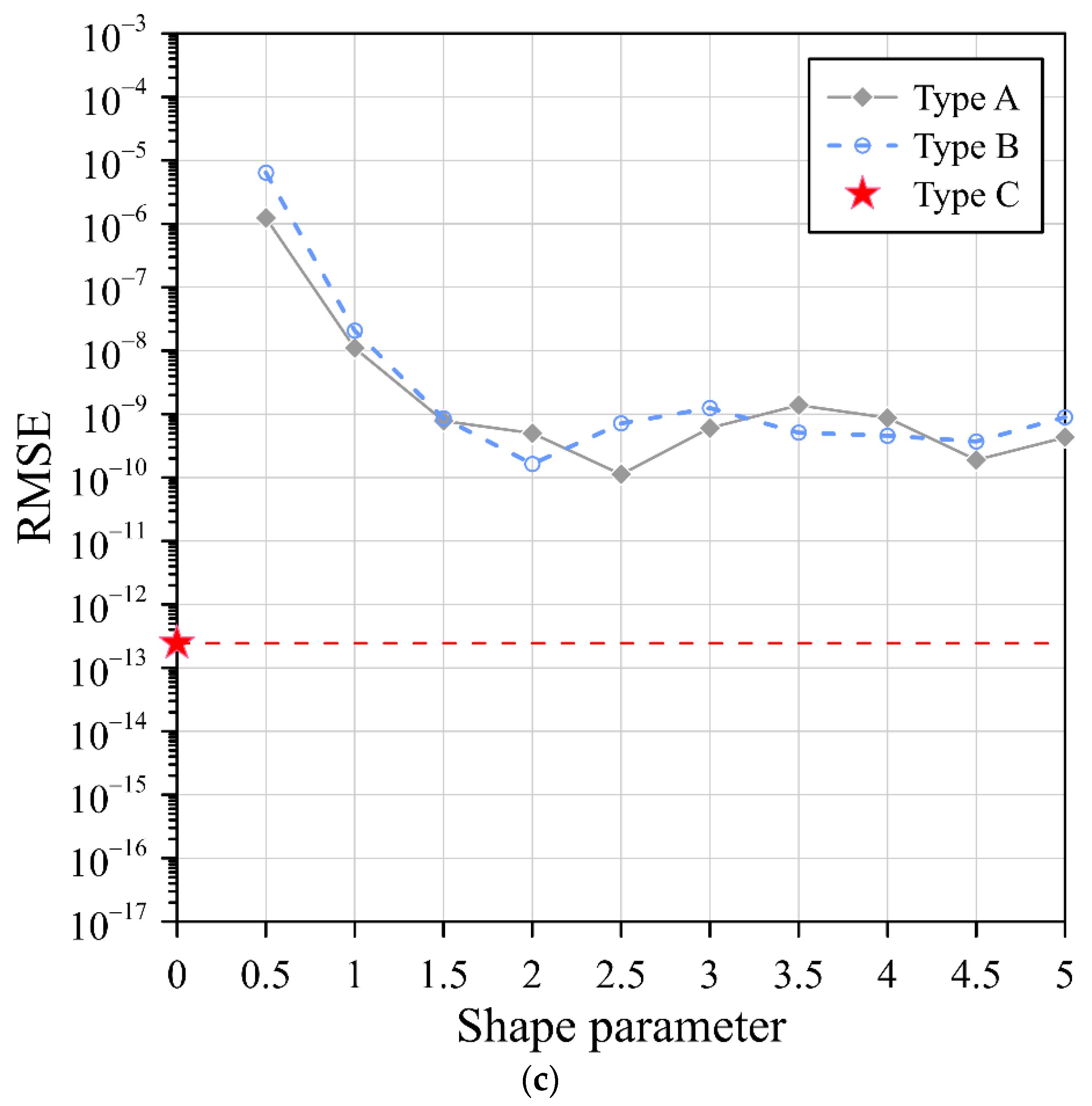
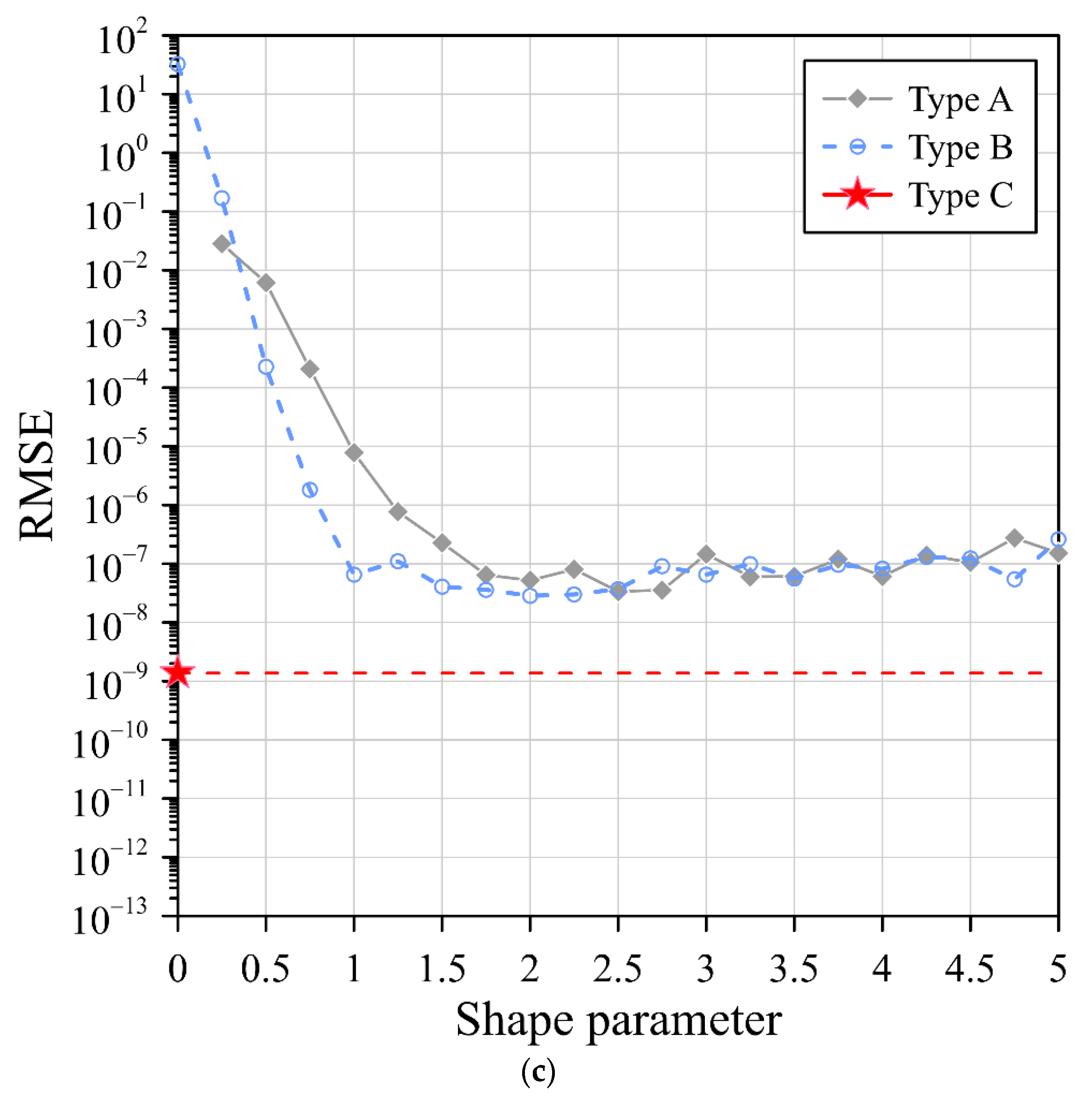
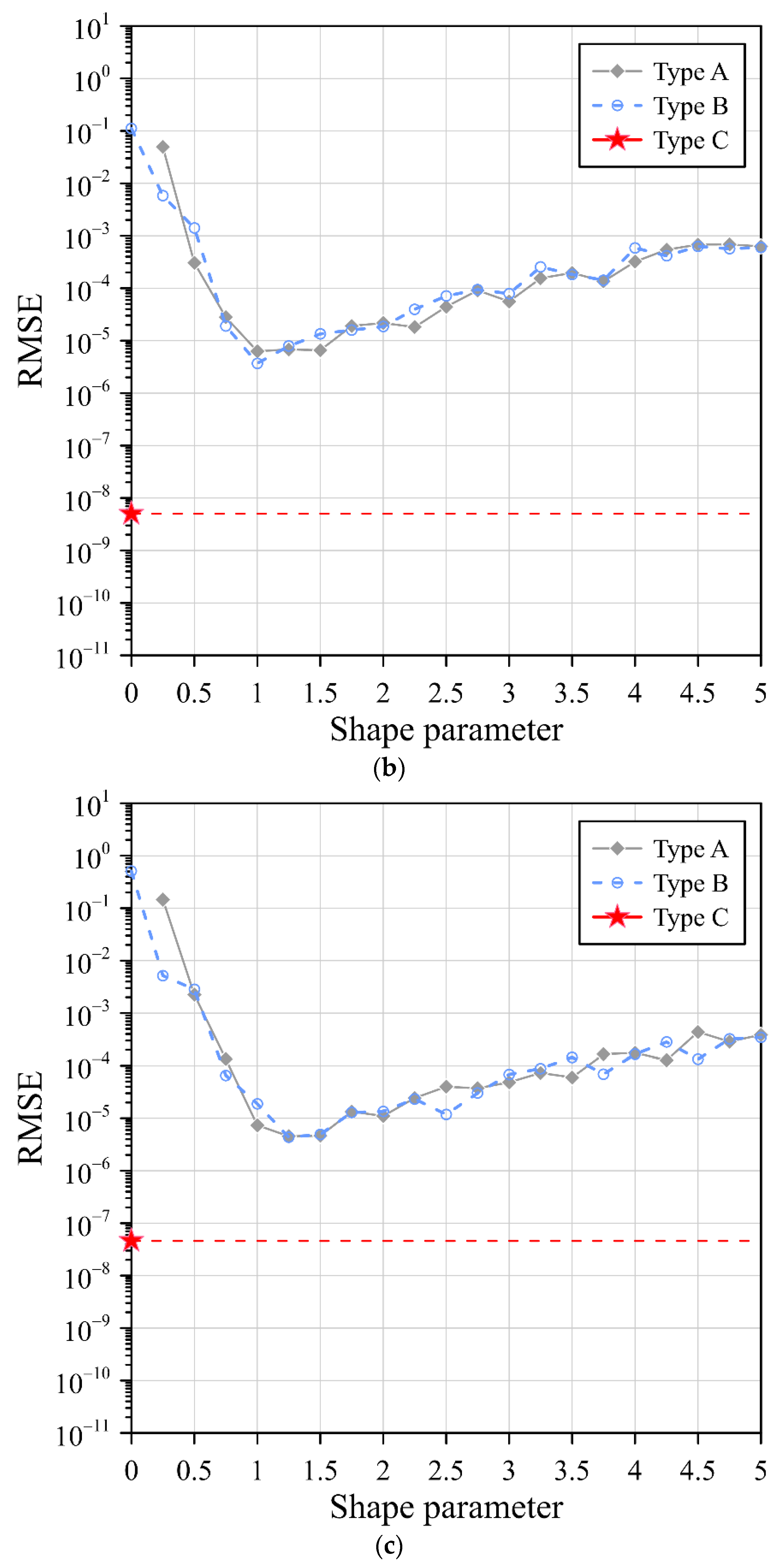
3.1.1. The Gaussian RBF
3.1.2. The MQ RBF
3.1.3. The IMQ RBF
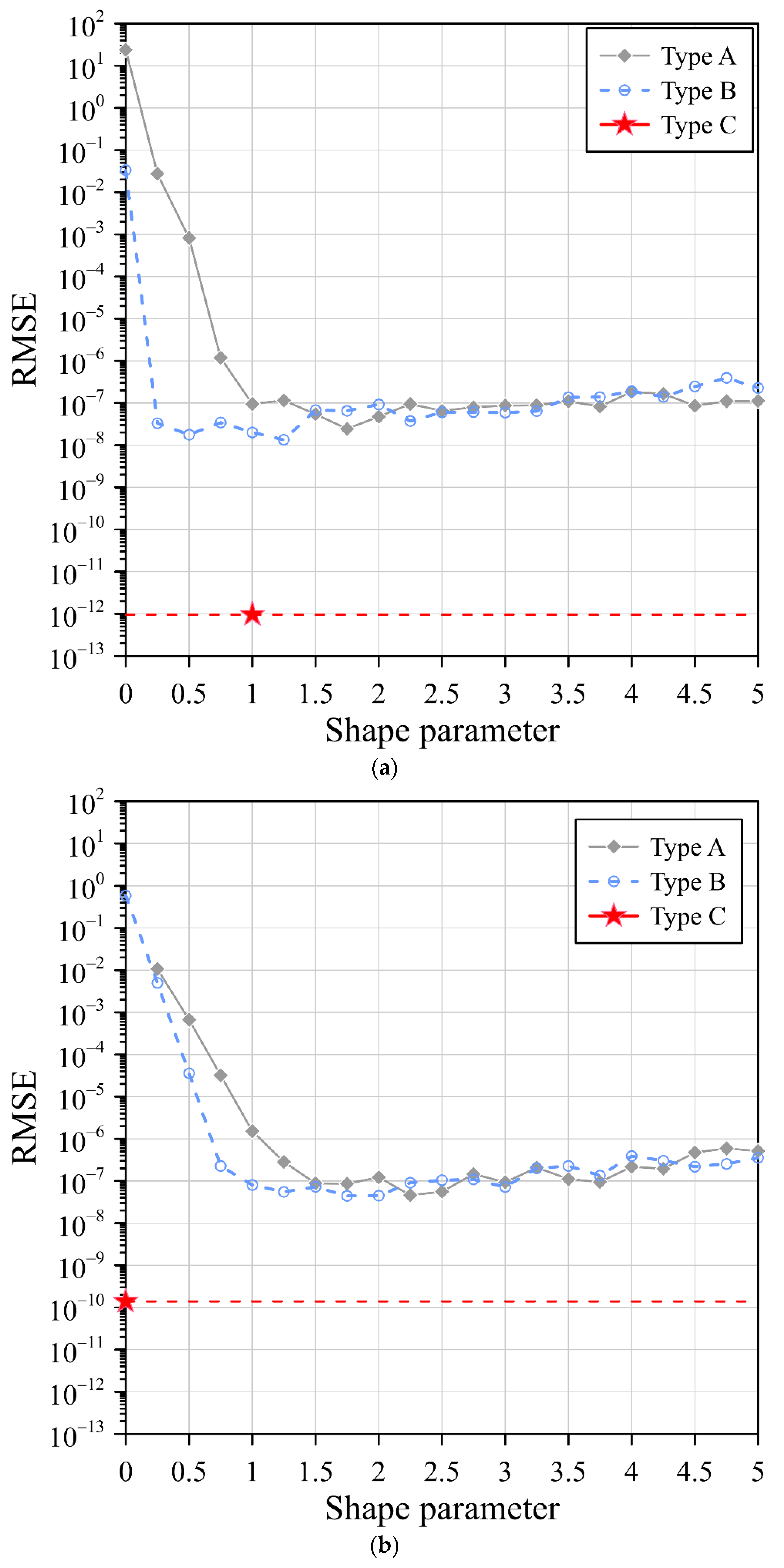
3.2. Example 2
4. Application Examples
4.1. Application Example 1
4.2. Application Example 2
4.3. Application Example 3
5. Conclusions
- (1)
- In this study, we demonstrated that the simplified RBFs, which consider many exterior fictitious sources outside the domain, can achieve accurate results to solve elliptic boundary value problems. The obtained results demonstrate that the simplified RBFs obtain a better accuracy than the original RBFs with the optimum shape parameter when solving elliptic boundary value problems.
- (2)
- Identification of the shape parameter is often very challenging and tedious in the original RBFs when solving partial differential equations. In this study, we proposed three simplified Gaussian, MQ, and IMQ RBFs without the shape parameter. The simplified RBFs have the advantages of a simple mathematical expression, high precision, and easy implementation.
- (3)
- With the consideration of many exterior fictitious sources outside the domain, we found that the radial distance is always greater than zero. The simplified Gaussian, MQ, and IMQ RBFs and their derivatives in the governing equation are always smooth and nonsingular.
- (4)
- Comparative analysis was conducted on the three different collocation types considering conventional uniform centers, randomly fictitious centers, and exterior fictitious sources. It was found that the exterior fictitious sources proposed in this study significantly improved the accuracy when solving problems.
- (5)
- Numerical examples, including elliptic BVPs in two and three dimensions, were carried out. The simplified radial basis function method with exterior fictitious sources can be applied to three-dimensional problems with ease and high accuracy.
- (6)
- In this study, we attempted to remove the shape parameter in conventional RBFs to solve partial differential equations. We achieved a promising result for three simplified Gaussian, MQ, and IMQ RBFs, especially for solving Laplace-type equations in two and three dimensions. Further studies to investigate the characteristics of the proposed method to solve different kinds of PDEs are suggested.
Author Contributions
Funding
Institutional Review Board Statement
Informed Consent Statement
Data Availability Statement
Conflicts of Interest
References
- Sanyasiraju, Y.V.S.S.; Chandhini, G. A note on two upwind strategies for RBF-based grid-free schemes to solve steady convection–diffusion equations. Int. J. Numer. Methods Fluids 2009, 61, 1053–1062. [Google Scholar] [CrossRef]
- Stevens, D.; Power, H.; Lees, M.; Morvan, H. The use of PDE centres in the local RBF Hermitian method for 3D convective-diffusion problems. J. Comput. Phys. 2009, 228, 4606–4624. [Google Scholar] [CrossRef]
- Wang, F.; Wang, C.; Chen, Z. Local knot method for 2D and 3D convection–diffusion–reaction equations in arbitrary domains. Appl. Math. Lett. 2020, 105, 106308. [Google Scholar] [CrossRef]
- Gu, Y. Meshfree methods and their comparisons. Int. J. Comput. Methods 2005, 2, 477–515. [Google Scholar] [CrossRef]
- Grabski, J.K. On the sources placement in the method of fundamental solutions for time-dependent heat conduction problems. Comput. Math. Appl. 2021, 88, 33–51. [Google Scholar] [CrossRef]
- Ku, C.Y.; Liu, C.Y.; Xiao, J.E.; Hsu, S.M.; Yeih, W. A collocation method with space–time radial polynomials for inverse heat conduction problems. Eng. Anal. Bound. Elem. 2020, 122, 117–131. [Google Scholar] [CrossRef]
- Cheng, A.H.-D. Particular solutions of Laplacian, Helmholtz-type, and polyharmonic operators involving higher order radial basis functions. Eng. Anal. Bound. Elem. 2000, 24, 531–538. [Google Scholar] [CrossRef]
- Hu, H.Y.; Li, Z.C.; Cheng, A.H.-D. Radial basis collocation methods for elliptic boundary value problems. Comput. Math. Appl. 2005, 50, 289–320. [Google Scholar] [CrossRef] [Green Version]
- Hardy, R.L. Multiquadric equations of topography and other irregular surfaces. J. Geophys. Res. 1971, 76, 1905–1915. [Google Scholar] [CrossRef]
- Kansa, E.J. Multiquadrics—A scattered data approximation scheme with applications to computational fluid-dynamics. II Solutions to parabolic, hyperbolic and elliptic partial-differential equations. Comput. Math. Appl. 1990, 19, 147–161. [Google Scholar] [CrossRef] [Green Version]
- Beatson, R.K.; Light, W.A. Fast evaluation of radial basis functions: Methods for two-dimensional polyharmonic splines. IMA J. Numer. Anal. 1997, 17, 343–372. [Google Scholar] [CrossRef]
- Santos, L.G.C.; Manzanares-Filho, N.; Menon, G.J.; Abreu, E. Comparing RBF-FD approximations based on stabilized Gaussians and on polyharmonic splines with polynomials. Int. J. Numer. Methods Eng. 2018, 115, 462–500. [Google Scholar] [CrossRef]
- Soleymani, F.; Barfeie, M.; Haghani, F.K. Inverse multiquadric RBF for computing the weights of FD method: Application to American options. Commun. Nonlinear Sci. Numer. Simul. 2018, 64, 74–88. [Google Scholar] [CrossRef]
- Liu, G. An overview on meshfree methods: For computational solid mechanics. Int. J. Comput. Methods 2016, 13, 1630001. [Google Scholar] [CrossRef]
- Uddin, M. RBF-PS scheme for solving the equal width equation. Appl. Math. Comput. 2013, 222, 619–631. [Google Scholar] [CrossRef]
- Liu, C.S.; Chang, C.W. An energy regularization of the MQ-RBF method for solving the Cauchy problems of diffusion-convection-reaction equations. Commun. Nonlinear Sci. Numer. Simul. 2019, 67, 375–390. [Google Scholar] [CrossRef]
- Ku, C.Y.; Hong, L.D.; Liu, C.Y.; Xiao, J.E. Space–time polyharmonic radial polynomial basis functions for modeling saturated and unsaturated flows. Eng. Comput. 2021, 1–14. [Google Scholar] [CrossRef]
- Fornberg, B.; Wright, G. Stable computation of multiquadric interpolants for all values of the shape parameter. Comput. Math. Appl. 2004, 48, 853–867. [Google Scholar] [CrossRef] [Green Version]
- Chen, W.; Hong, Y.; Lin, J. The sample solution approach for determination of the optimal shape parameter in the Multiquadric function of the Kansa method. Comput. Math. Appl. 2018, 75, 2942–2954. [Google Scholar] [CrossRef]
- Cavoretto, R.; De Rossi, A. Adaptive procedures for meshfree RBF unsymmetric and symmetric collocation methods. Appl. Math. Comput. 2020, 382, 125354. [Google Scholar] [CrossRef]
- Issa, K.; Humbali, K.M.; Biazar, J. An algorithm for choosing best shape parameter for numerical solution of partial differential equation via inverse multiquadric radial basis function. Open J. Math. Sci. 2020, 4, 147–157. [Google Scholar] [CrossRef]
- Zhang, J.; Wang, F.Z.; Hou, E.R. The conical radial basis function for partial differential equations. J. Math. 2020, 2020, 6664071. [Google Scholar] [CrossRef]
- Katsiamis, A.; Karageorghis, A. Kansa radial basis function method with fictitious centres for solving nonlinear boundary value problems. Eng. Anal. Bound. Elem. 2020, 119, 293–301. [Google Scholar] [CrossRef]
- Liu, C.Y.; Ku, C.Y.; Hong, L.D.; Hsu, S.M. Infinitely smooth polyharmonic RBF collocation method for numerical solution of elliptic PDEs. Mathematics 2021, 9, 1535. [Google Scholar] [CrossRef]
- Ku, C.Y.; Liu, C.Y.; Xiao, J.E.; Hsu, S.M. Multiquadrics without the shape parameter for solving partial differential equations. Symmetry 2020, 12, 1813. [Google Scholar] [CrossRef]
- Yue, X.; Jiang, B.; Xue, X.; Yang, C. A Simple, Accurate and Semi-Analytical Meshless Method for Solving Laplace and Helmholtz Equations in Complex Two-Dimensional Geometries. Mathematics 2022, 10, 833. [Google Scholar] [CrossRef]


| Type of RBFs | Original RBFs | Simplified RBFs |
|---|---|---|
| Gaussian | ||
| Multiquadric (MQ) | ||
| Inverse multiquadric (IMQ) |
| RBF | RMSE | ||
|---|---|---|---|
| Type A | Type B | Type C () | |
| Gaussian | 1.24 × 10⁻⁷ | 9.73 × 10⁻⁸ | 7.87 × 10⁻¹² |
| () | () | () | |
| (t = 5.84 s) | (t = 4.62 s) | (t = 8.11 s) | |
| MQ | 1.42 × 10⁻⁷ | 1.46 × 10⁻⁷ | 4.35 × 10⁻¹³ |
| () | () | () | |
| (t = 5.78 s) | (t = 5.75 s) | (t = 7.96 s) | |
| IMQ | 1.47 × 10⁻⁷ | 8.46 × 10⁻⁸ | 6.37 × 10⁻¹² |
| () | () | () | |
| (t = 6.12 s) | (t = 6.28 s) | (t = 8.51 s) | |
| RBF | RMSE | ||
|---|---|---|---|
| Type A | Type B | Type C () | |
| Gaussian | 2.45 × 10⁻⁸ | 1.33 × 10⁻⁸ | 9.50 × 10⁻¹³ |
| () | () | () | |
| (t = 3.82 s) | (t = 7.02 s) | (t = 8.81 s) | |
| MQ | 4.61 × 10⁻⁸ | 4.41 × 10⁻⁸ | 1.39 × 10⁻¹⁰ |
| () | () | () | |
| (t = 3.80 s) | (t = 6.90 s) | (t = 8.77 s) | |
| IMQ | 3.38 × 10⁻⁸ | 2.85 × 10⁻⁸ | 1.37 × 10⁻⁹ |
| () | () | () | |
| (t = 3.80 s) | (t = 6.99 s) | (t = 8.83 s) | |
| RBF | RMSE | ||
|---|---|---|---|
| Type A | Type B | Type C ( | |
| Gaussian | 1.18 × 10⁻⁶ | 1.61 × 10⁻⁶ | 2.76 × 10⁻¹¹ |
| () | () | () | |
| (t = 7.24 s) | (t = 9.47 s) | (t = 12.57 s) | |
| MQ | 6.28 × 10⁻⁶ | 3.70 × 10⁻⁶ | 5.04 × 10⁻⁹ |
| () | () | () | |
| (t = 7.28 s) | (t = 10.34 s) | (t = 13.01 s) | |
| IMQ | 4.54 × 10⁻⁶ | 4.32 × 10⁻⁶ | 4.59 × 10⁻⁸ |
| () | () | () | |
| (t = 7.24 s) | (t = 11.67 s) | (t = 12.67 s) | |
Publisher’s Note: MDPI stays neutral with regard to jurisdictional claims in published maps and institutional affiliations. |
© 2022 by the authors. Licensee MDPI, Basel, Switzerland. This article is an open access article distributed under the terms and conditions of the Creative Commons Attribution (CC BY) license (https://creativecommons.org/licenses/by/4.0/).
Share and Cite
Liu, C.-Y.; Ku, C.-Y. A Simplified Radial Basis Function Method with Exterior Fictitious Sources for Elliptic Boundary Value Problems. Mathematics 2022, 10, 1622. https://doi.org/10.3390/math10101622
Liu C-Y, Ku C-Y. A Simplified Radial Basis Function Method with Exterior Fictitious Sources for Elliptic Boundary Value Problems. Mathematics. 2022; 10(10):1622. https://doi.org/10.3390/math10101622
Chicago/Turabian StyleLiu, Chih-Yu, and Cheng-Yu Ku. 2022. "A Simplified Radial Basis Function Method with Exterior Fictitious Sources for Elliptic Boundary Value Problems" Mathematics 10, no. 10: 1622. https://doi.org/10.3390/math10101622