Article

Largest Lyapunov Exponent Parameter of Stiffened Carbon Fiber Reinforced Epoxy Composite Laminated Plate Due to Critical Buckling Load Using Average Logarithmic Divergence Approach

Department of Mechanical Engineering, San Diego State University, 5500 Campanile Drive, San Diego, CA 92182-1323, USA
Mathematics 2022, 10(12), 2020; https://doi.org/10.3390/math10122020
Submission received: 12 April 2022 / Revised: 2 June 2022 / Accepted: 7 June 2022 / Published: 11 June 2022

Abstract

:
The purpose of this study is to calculate the bending deflection which is used to investigate the largest Lyapunov exponent due to buckling load. The design methodology is to calculate the largest Lyapunov exponent parameter at different thickness ratios and different fiber volume fractions using one and two stiffeners in order to reduce the chaotic phenomenon. The practical implication is to find the bending deflection using a strain gauge through a strain meter, in which this bending deflection is used in the algorithm of average logarithmic divergence to calculate the largest Lyapunov exponent experimentally. The experiment set up is carried out using Southwell plot when the upper head of the servo hydraulic cylinder moves downward. There are no limitations to this research, since it works on all kinds of composite materials, different thickness ratios, and different number of layers, different fiber volume fractions, and different boundary conditions. The findings of this work will allow us to detect the chaotic phenomenon in a stiffened carbon fiber reinforced epoxy composite laminated plate using the conception of the largest Lyapunov exponent parameter. The higher order shear deformation theory (HOSDT) of plates is used to analytically calculate the set of data of the bending deflection against time. All the systems used in this paper have non-periodic motion and chaos because the value of the Lyapunov parameter is above zero. The originality of this paper is the use of the algorithm code of average logarithmic divergence to investigate the value of the largest Lyapunov exponent parameter in the presence of stiffeners based on the bending deflection of a carbon epoxy composite laminated plate.

1. Introduction

The nonlinear dynamics phenomenon is the most critical mode for failure; predicting the buckling loads of thin carbon fiber reinforced epoxy composite plates is extremely important in parametric design. The application of this work can be used in spaceships and steam boilers. Lal et al. presented thermal post buckling in a sandwich composite laminated plate using shape memory alloys under uniform temperature distribution. They used the higher order shear deformation theory with von Karman nonlinear kinematics by the finite element method to investigate the critical buckling temperature [1]. Yousuf studied the nonlinear dynamics behavior of the bending deflection in a composite laminated plate using the conception of the largest Lyapunov exponent parameter. The non-periodic motion and chaos was investigated using Fast Fourier Transform (FFT) at different fiber volume fractions and different aspect ratios. He concluded that the non-periodic motion of the bending deflection decreases with the increase in aspect ratios, while the non-periodic motion of the bending deflection is increased with the increase in fiber volume fractions [2]. Mondal and Ramachandra computed the dynamic buckling load using Tsai-Wu quadratic criterion, in which the nonlinear dynamics phenomena is investigated at different pulse type of buckling. The response of the delaminated composite plate is calculated at different types of pulse loading such as sinusoidal, exponential and rectangular [3]. Keshav and Patel studied the nonlinear dynamic buckling of a laminated composite curved panel under dynamic in-plane axial compressive load using the finite element method. They studied the effect of aspect ratio, radius of curvature and thickness on the dynamic buckling load [4]. Moreover, Keshav et al. calculated the dynamic buckling load using Volmir’s criterion, while the nonlinear dynamic equations were solved using the finite element method [5]. Balkan et al. studied the effect of the sandwich stiffener on the nonlinear dynamic behavior of the composite laminated plate under non-uniform blast load. They calculated the displacement, strain and stress in order to investigate the dynamic response of the stiffener after solving the nonlinear coupled equations using the NDSOLVE function of Mathematica Software, [6]. Yousuf reduced the nonlinear linear dynamics behavior of the composite laminated plate using a beam stiffener. The combined loading included the in-plane compression mechanical load and shear force. He concluded that all the values of the largest Lyapunov exponent were positive, indicating non-periodic motion and chaos [7]. Many studies have not taken into consideration the use of the largest Lyapunov exponent parameter of the algorithm of average logarithmic divergence and Fast Fourier Transform of power density function in the investigation of non-periodic motion and chaos. The aim of this article is to study the nonlinear dynamics behavior of a stiffened carbon fiber reinforced epoxy composite laminated plate due to critical buckling load. The largest Lyapunov exponent is calculated for the composite plate, with and without stiffeners, at different thickness ratios and different fiber volume fractions.

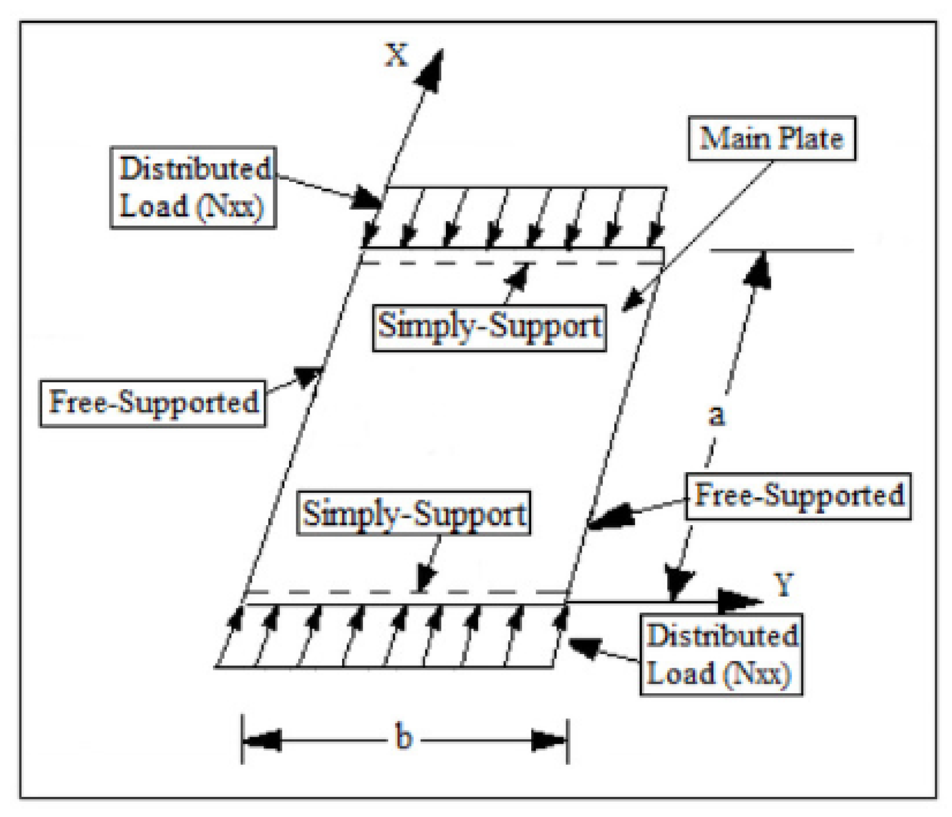
2. Analytic Solution of the Bending Deflection

The higher order shear deformation plate theory assumes that the straight line (perpendicular to the mid surface) before deformation becomes a curve line after deformation [8]:
u ( x , y , z , t ) = u o ( x , y , t ) + z   x ( x , y , t ) 4 3 h 2 z 3 ( x + w 0 x )
v ( x , y , z , t ) = v o ( x , y , t ) + z   y ( x , y , t ) 4 3 h 2 z 3 ( y + w 0 y )
w ( x , y , z , t ) =   w o ( x , y , t )
The transformed stress–strain relations of an orthotropic lamina in a plane state of stress for the un-stiffened plate are illustrated in the following equation [8]:
{ σ xx σ yy σ xy } k = [ Q ¯ 11 Q ¯ 12 Q ¯ 16 Q ¯ 12 Q ¯ 22 Q ¯ 26 Q ¯ 16 Q ¯ 26 Q ¯ 66 ] k { ε xx   ε yy γ xy }
{ σ yz σ xz } k = [ Q ¯ 44 Q ¯ 45 Q ¯ 45 Q ¯ 55 ] { γ yz γ xz }
where:
{ ε xx ε yy γ xy } = { ε xx ( 0 ) ε yy ( 0 ) γ xy ( 0 ) } + z   { ε xx ( 1 ) ε yy ( 1 ) γ xy ( 1 ) } +   z 3 { ε xx ( 3 ) ε yy ( 3 ) γ xy ( 3 ) }
{ γ yz γ xz } = { γ yz ( 0 ) γ xz ( 0 ) } + z { γ yz ( 1 ) γ xz ( 1 ) } +   z 2 { γ yz ( 2 ) γ xz ( 2 ) }
The stress–strain relations for the stiffeners are as shown below [9]:
σ xx ) st   =   E x st · Ԑ xx σ yy ) st   =   E y st · Ԑ yy τ xy )   st = 0 τ yz )   st = G y st · γ yz τ xz )   st = G x st · γ xz    
where:
σ xx , σ yy : Normal stress of the stiffeners in the (x) and (y) directions.
τ xy , τ yz , τ xz : Shear stresses of the stiffeners in (xy), (yz), and (xz) planes.
Ԑ xx , Ԑ yy : Strains of the stiffeners along (x) and (y) directions.
E x st , E y st : Modulus of elasticity of the stiffeners along (x) and (y) directions.
G x st . and G y st . are the shear modulus of elasticity of stiffeners along (x and y) directions.
γ yz , γ xz : Shear strain of the stiffeners along (x) and (y) directions.
The force and moment relations of the plate in the presence of the stiffener are indicated in the following equation:
[ N M P ] = [ N M P ] unst + [ N M P ] st
[ Q R ] = [ Q R ] unst + [ Q R ] st
where:
{ N xx N yy N xy } unst . = [ A 11 A 12 A 16 A 12 A 22 A 26 A 16 A 26 A 66 ] { ε xx 0 ε yy 0 γ xy 0 } + [ B 11 B 12 B 16 B 12 B 22 B 26 B 16 B 26 B 66 ] { ε xx 1 ε yy 1 γ xy 1 } c 1 [ E 11 E 12 E 16 E 12 E 22 E 26 E 16 E 26 E 66 ] { ε xx ( 3 ) ε yy ( 3 ) γ xy ( 3 ) }
and,
{ M xx M yy M xy } unst . = [ B 11 B 12 B 16 B 12 B 22 B 26 B 16 B 26 B 66 ] { ε xx 0 ε yy 0 γ xy 0 } + [ D 11 D 12 D 16 D 12 D 22 D 26 D 16 D 26 D 66 ] { ε xx 1 ε yy 1 γ xy 1 }   c 1 [ F 11 F 12 F 16 F 12 F 22 F 26 F 16 F 26 F 66 ] { ε xx ( 3 ) ε yy ( 3 ) γ xy ( 3 ) }
Also
{ P xx P yy P xy } unst . = [ E 11 E 12 E 16 E 12 E 22 E 26 E 16 E 26 E 66 ] { ε xx 0 ε yy 0 γ xy 0 } + [ F 11 F 12 F 16 F 12 F 22 F 26 F 16 F 26 F 66 ] { ε xx 1 ε yy 1 γ xy 1 } c 1 [ H 11 H 12 H 16 H 12 H 22 H 26 H 16 H 26 H 66 ] { ε xx ( 3 ) ε yy ( 3 ) γ xy ( 3 ) }
{ Q yz Q xz }   unst . = [ A 44 A 45 A 45 A 55 ] { γ yz ( 0 ) γ xz ( 0 ) } c 2 [ D 44 D 45 D 45 D 55 ] { γ yz ( 2 ) γ xz ( 2 ) } { R yz R xz }   unst . = [ D 44 D 45 D 45 D 55 ] { γ yz ( 0 ) γ xz ( 0 ) } c 2 [ F 44 F 45 F 45 F 55 ] { γ yz ( 2 ) γ xz ( 2 ) }
where
A ij ,   B ij ,   D ij ,   E ij ,   F ij ,   H ij = k = 1 N z k z k   + 1 Q ¯ ij ( k ) ( 1 ,   z ,   z 2 , z 3 , z 4 , z 6 )   dz
For the stiffened plate, the force and moment are illustrated in the following equations [8]:
[ N xx N yy M xx M yy P x P y ] st = [ A 11 st 0 0 A 22 st B 11 st 0 0   B 22 st E 11 st 0 0 E 22 st ] [ ε xx ε yy ]
[ Q yz Q xz R yz R xz ] st = [ A 44 st 0 0 A 55 st D 44 st 0 0 D 55 st ] [ γ yz γ xz ]
where:
( A 11 st , B 22 st , D 11 st , E 11 st ) = Zi 1 ) x st Zi ) x st tx bx     Ex st     ( 1 , Z , Z 2 , Z 3 ) · dZ      
( A 11 st , B 22 st , D 11 st , E 11 st ) = Zi 1 ) y st Zi ) y st ty by     Ey st     ( 1 , Z , Z 2 , Z 3 ) · dZ      
and
A 44 st = Zi 1 ) y st Zi ) y st Gy st     ty by     dZ
A 55 st = Zi 1 ) x st Zi ) x st   Gx st     tx bx     dZ
D 44 st = Zi 1 ) y st Zi ) y st Gy st     ty by     Z 2   dZ
D 55 st = Zi 1 ) x st Zi ) x st   Gx st     tx bx     Z 2     dZ

3. Equations of Motion

The Euler-Lagrange equations are obtained by setting the coefficient of (δ u o , δ v o , δ w o , δ Ø x and δ Ø y ) to zero separately [8]:
N xx x + N xy y = 0  
N xy x + N yy y = 0
Q x x c 2 R x x + Q y y c 2 R y y +   c 1   ( 2 P xx x 2 + 2 2 P xy x   y + 2 P yy y 2 ) + N ^ xx 2 w x 2 + N ^ yy 2 w y 2 + 2 N ^ xy 2 w x y = 0  
M xx x c 1 P xx x + M xy y c 1 P xy y Q x +   c 2 R x = 0
M xy x c 1 P xy x + M yy y c 1 P yy y Q y +   c 2 R y = 0
The loading and boundary conditions can be seen in Figure 1, while the composite plate with different stiffeners is indicated in Figure 2.

4. Solution of Analytic Equation of Motion

The general solution is illustrated in the following equation:
[ K ] [ Δ ] = [ F ]
where:
[ K ] = [ L Unstiffened ] + [ L stiffened ]
[ Δ ] = [ u o , v o ,   w o , Q x   , Q y ]
[ F ] = [ 0 , 0 , 0 , 0 , 0 ]
The system of equations may be converted to the first order differential operator form:
Z X =   A     Z
Z   =   e AX     K
K is the column vector of constants to be determined from the edge conditions.
e AX = [ S ] [ e λ 1 X 0 0 e λ n X ] [ S ] 1
where:
n = 12.
λ ns is the Eigen value of [ A s ].
[S] is the matrix of Eigen vector of [ A s ].

4.1. Solution of Equation of Motion of Unstiffened Plate

The Lagrange coefficients of the stiffness matrix due to δ u o , δ v o , δ w o , δ Ø x and δ Ø y for unstiffened plate are as in below:
L 11 =   A 11 2 x 2 + 2 A 16 2 x y   + A 66 2 y 2 ,   L 12 = A 12 2 x y   +   A 16 2 x 2 + A 26 2 y 2 + A 66 2 x y ,   L 13   = c 1 [ E 11 3 x 3 + ( E 12 + 2 E 66 ) 2 y 2 x + ( 3 E 16 ) 2 x 2 y + E 26 3 y 3 ] L 14 = B 11 2 x 2 + B 16 2 x y c 1 E 11 2 x 2 2 c 1 E 16 2 x y + B 16 2 x y + B 66 2 y 2 c 1 E 16 2 x y c 1 E 66 2 y 2 ,   L 15 = B 12 2 x y + B 16 2 x 2 c 1 E 12 2 x y c 1 E 16 2 x 2 + B 26 2 y 2 + B 66 2 x y c 1 E 26 2 y 2 c 1 E 66 2 x y ,   L 22 = A 66 2 x 2 + A 22 2 y 2 + 2 A 26 2 x y ,   L 23 = c 1 E 16 3 x 3 3 c 1 E 26 2 y 2 x ( 2 c 1 E 66 + c 1 E 12 ) 2 x 2 y c 1 E 22 3 y 3 ,   L 24 = L 15 ,   L 25 = B 66 2 x 2 + B 26 2 x y c 1 E 26 2 x y c 1 E 66 2 x 2 + B 22 2 y 2 + B 26 2 x y c 1 E 22 2 y 2 c 1 E 26 2 x y , L 33   =   A 45 2 x y   +   A 55 2 x 2   c 2 D 45 2 x y   c 2 D 55 2 x 2   c 2 x ( D 45 y   + D 55 x   c 2 F 45 y   c 2 F 55 x )   + A 44 2 y 2   + A 45 2 x y   c 2 D 44 2 y 2   c 2 D 45 2 x y   c 2 y ( D 44 y   + D 45 x   c 2 F 44 y   c 2 F 45 x ) c 1 2 x 2 ( c 1 H 11 2 x 2   c 1 H 12 2 y 2     2 c 1 H 16 2 x y )   2 c 1 2 x y ( c 1 H 16 2 x 2   c 1 H 26 2 y 2     2 c 1 H 66 2 x y )   + c 1 2 y 2 ( c 1 H 12 2 x 2   c 1 H 22 2 y 2     2 c 1 H 26 2 x y ) + N xx 2 x 2   + N yy 2 y 2 L 34   =   A 55 x     2 c 2 D 55 x   + c 2 2 F 55 x   + A 45 y     2 c 2 D 45 y   + c 2 2 F 45 y   c 1 F 11 3 x 3   c 1 F 16 2 x 2 y   + c 1 2 H 11 3 x 3   + c 1 2 H 16 2 x 2 y     2 c 1 2 x y ( F 16 x   + F 66 y   c 1 H 16 x   c 1 H 66 y ) c 1 2 y 2 ( F 12 x   + F 26 y   c 1 H 12 x   c 1 H 26 y ) L 35   = A 45 x   c 2 D 45 x   c 2 x ( D 45   c 2 F 45 )   + A 44 y   c 2 D 44 y   c 2 y ( D 44   c 2 F 44 )   c 1 2 x 2 ( F 12 y   + F 16 x   c 1 H 12 y   c 1 H 16 x ) 2 c 1 2 x y ( F 26 y   + F 66 x   c 1 H 26 y   c 1 H 66 x )   c 1 2 y 2 ( F 22 y   + F 26 x   c 1 H 22 y   c 1 H 26 x ) L 44   =   x ( D 11 x   + D 16 y   c 1 F 11 x   c 1 F 16 y )   c 1 x ( F 11 x   + F 16 y   c 1 H 11 x c 1 H 16 y )   +   y ( D 16 x   + D 66 y   c 1 F 16 x   c 1 F 66 y )   c 1 y ( F 16 x   + F 66 y   c 1 H 16 x   c 1 H 66 y )   + A 55     2 c 2 D 55   + c 2 2 F 55 L 45   =   x ( D 12 y   + D 16 x   c 1 F 12 y   c 1 F 16 x )   c 1 x ( F 12 y   + F 16 x   c 1 H 12 y   c 1 H 16 x )   +   y ( D 26 y   + D 66 x   c 1 F 26 y   c 1 F 66 x )   c 1 y ( F 26 y   + F 66 x   c 1 H 26 y   c 1 H 66 x )   + A 45     2 c 2 D 45   + c 2 2 F 45 L 55   =   x ( D 26 y   + D 66 x   c 1 F 26 y   c 1 F 66 x )   c 1 x ( F 26 y   + F 66 x   c 1 H 26 y   c 1 H 66 x )   +   y ( D 22 y   + D 26 x   c 1 F 22 y   c 1 F 26 x )   c 1 y ( F 22 y   + F 26 x   c 1 H 22 y   c 1 H 26 x )   + A 44     2 c 2 D 44   + c 2 2 F 44 L 11 = A 11 x + A 66 y + 2 A 16 2 x y ,   L 12 = ( A 12 + A 66 ) 2 x y + A 16 x + A 26 y L 13 = c 1 [ E 11 3 x 3 + ( E 12 + 2 E 66 ) x 2 y 2 + 3 E 16 y 2 x 2 +   E 26 3 y 3 ] L 14 = ( B 11   c 1 E 11 ) 2 x 2 + ( B 66   c 1 E 66 ) 2 y 2 + 2 ( B 16   c 1 E 16 ) 2 x y L 15 = ( B 12   c 1 E 12 ) 2 x y + ( B 66   c 1 E 66 ) 2 x y + ( B 16   c 1 E 16 ) 2 x 2 + ( B 26   c 1 E 26 ) 2 y 2 L 22 =   A 66 2 x 2 +   A 22 2 y 2 + 2 A 26 2 x y L 23 = [ 2 c 1 E 66 +   c 1 E 12 ] 2 x 2 y   c 1 E 22 3 y 3   c 1 E 12 3 x 3 3 c 1 E 26 2 y 2 x L 24 = L 15 L 25 = ( B 66 c 1 E 66 ) 2 x 2 + ( B 22 c 1 E 22 ) 2 y 2 + 2 ( B 26 c 1 E 26 ) 2 x y

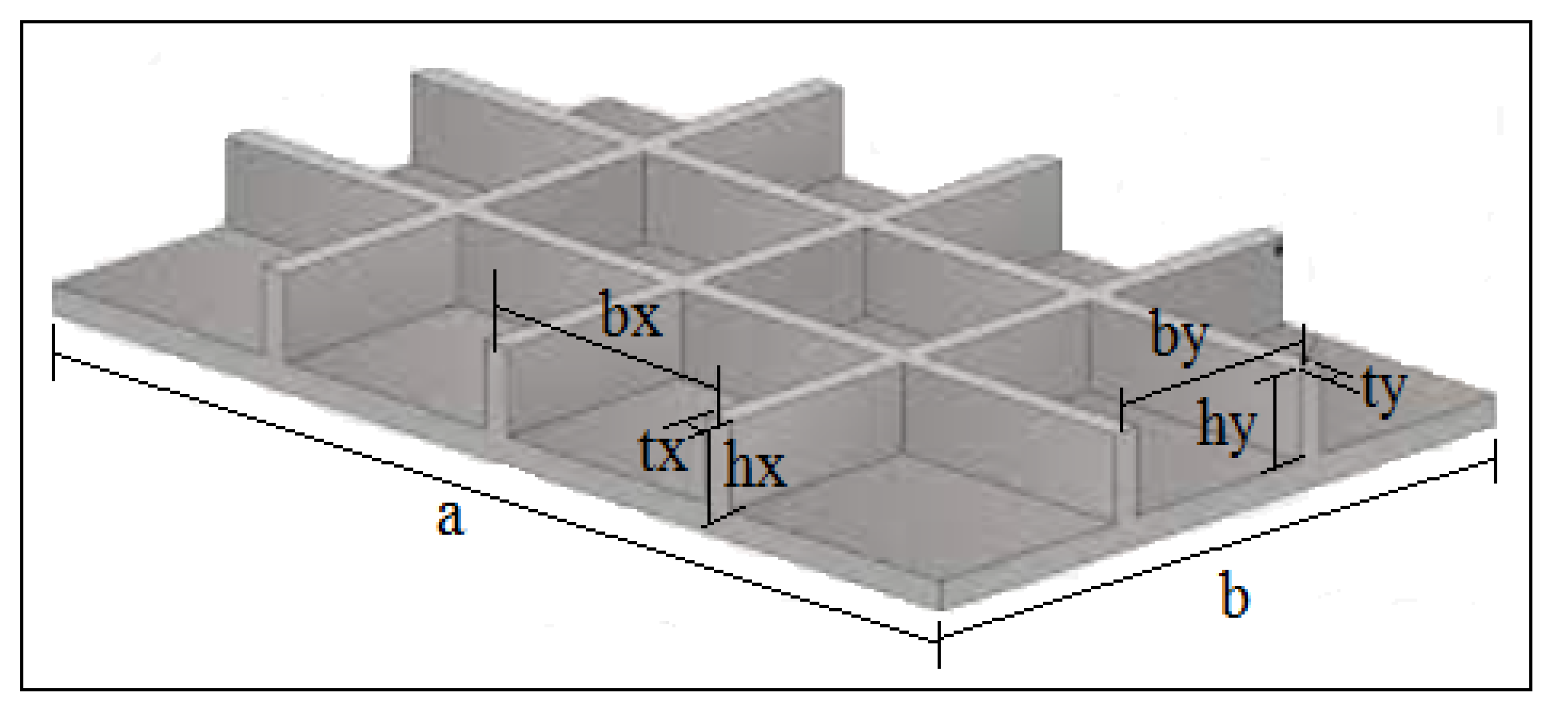
4.2. Solution of Equation of Motion of Stiffener
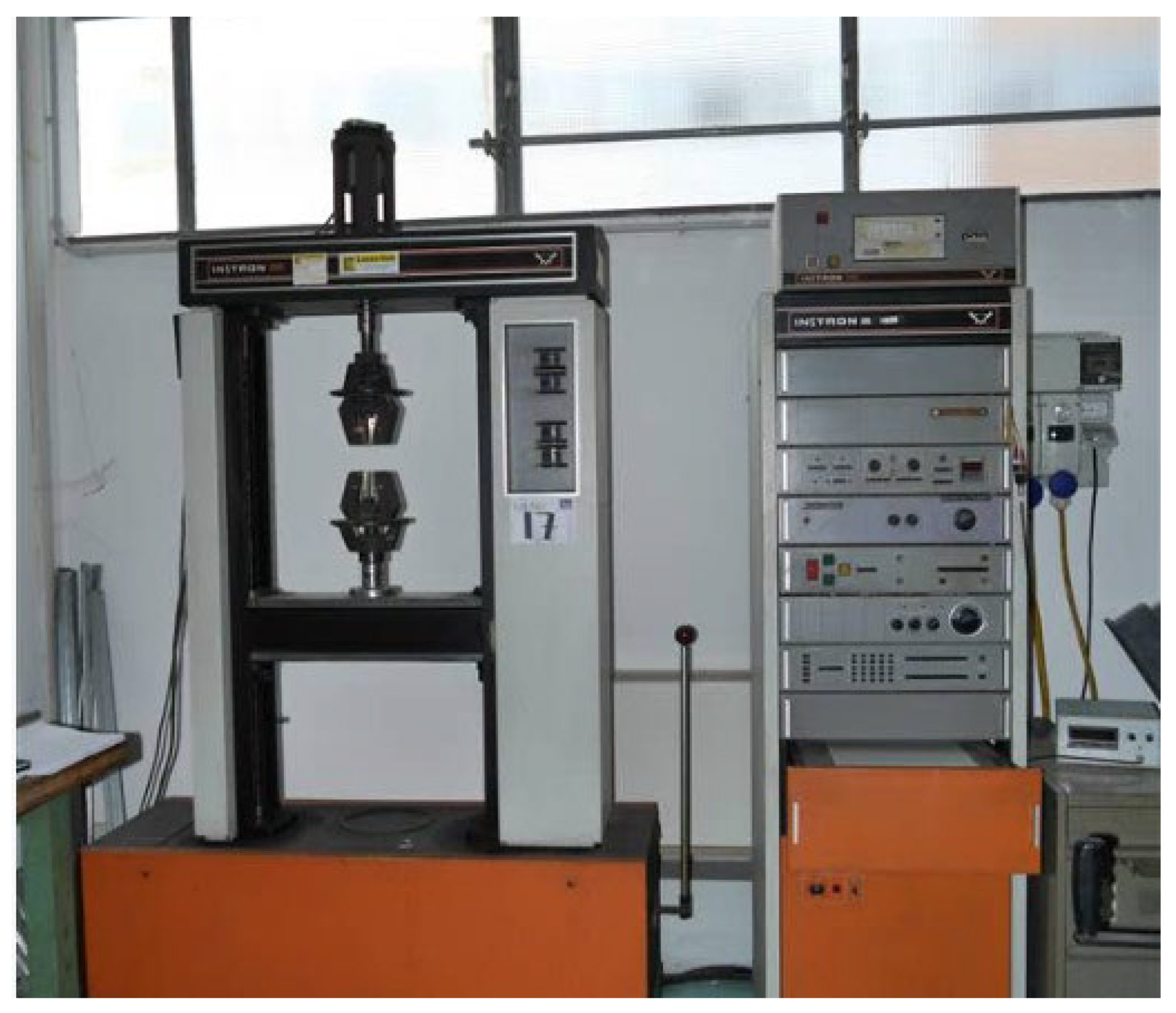
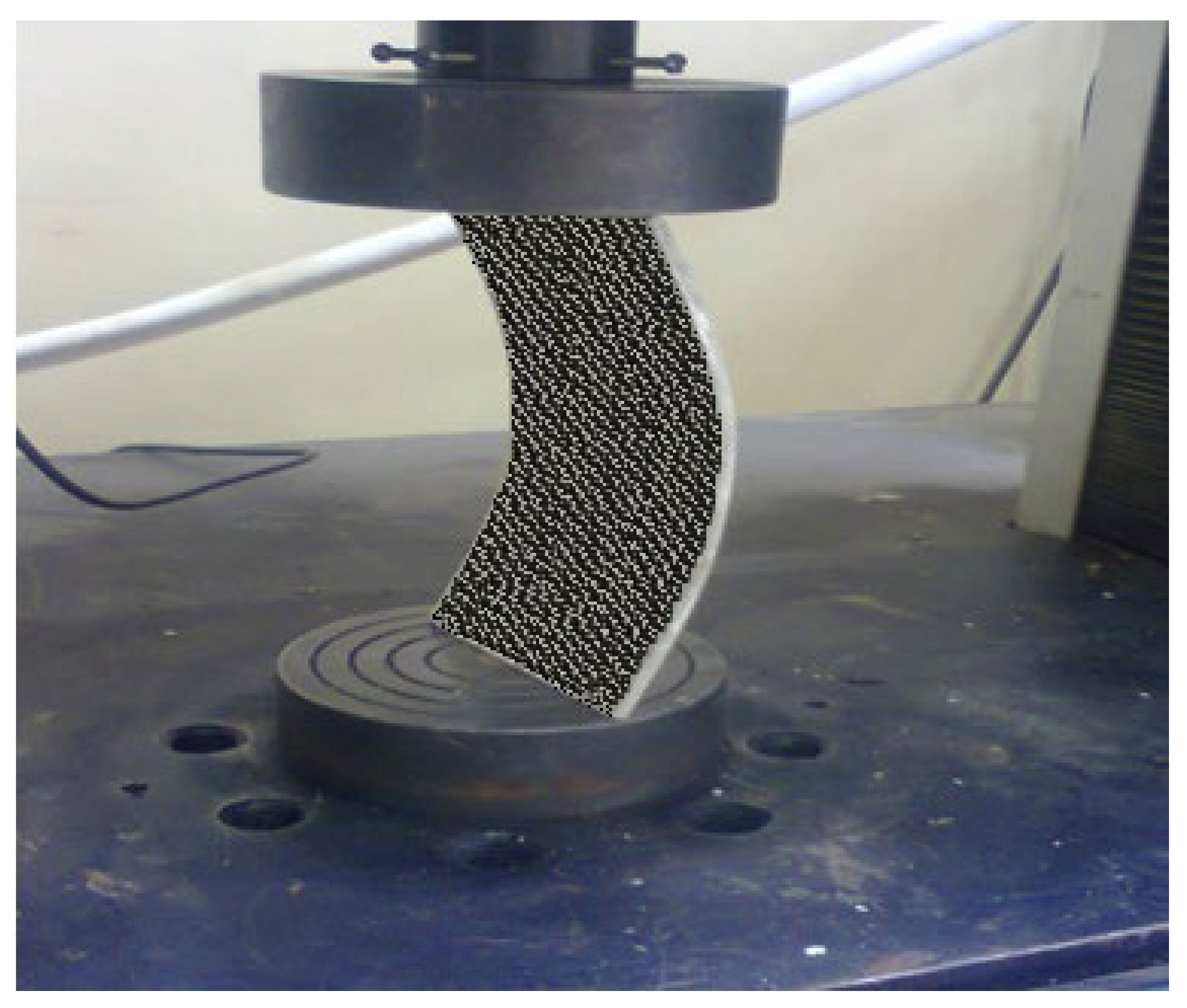
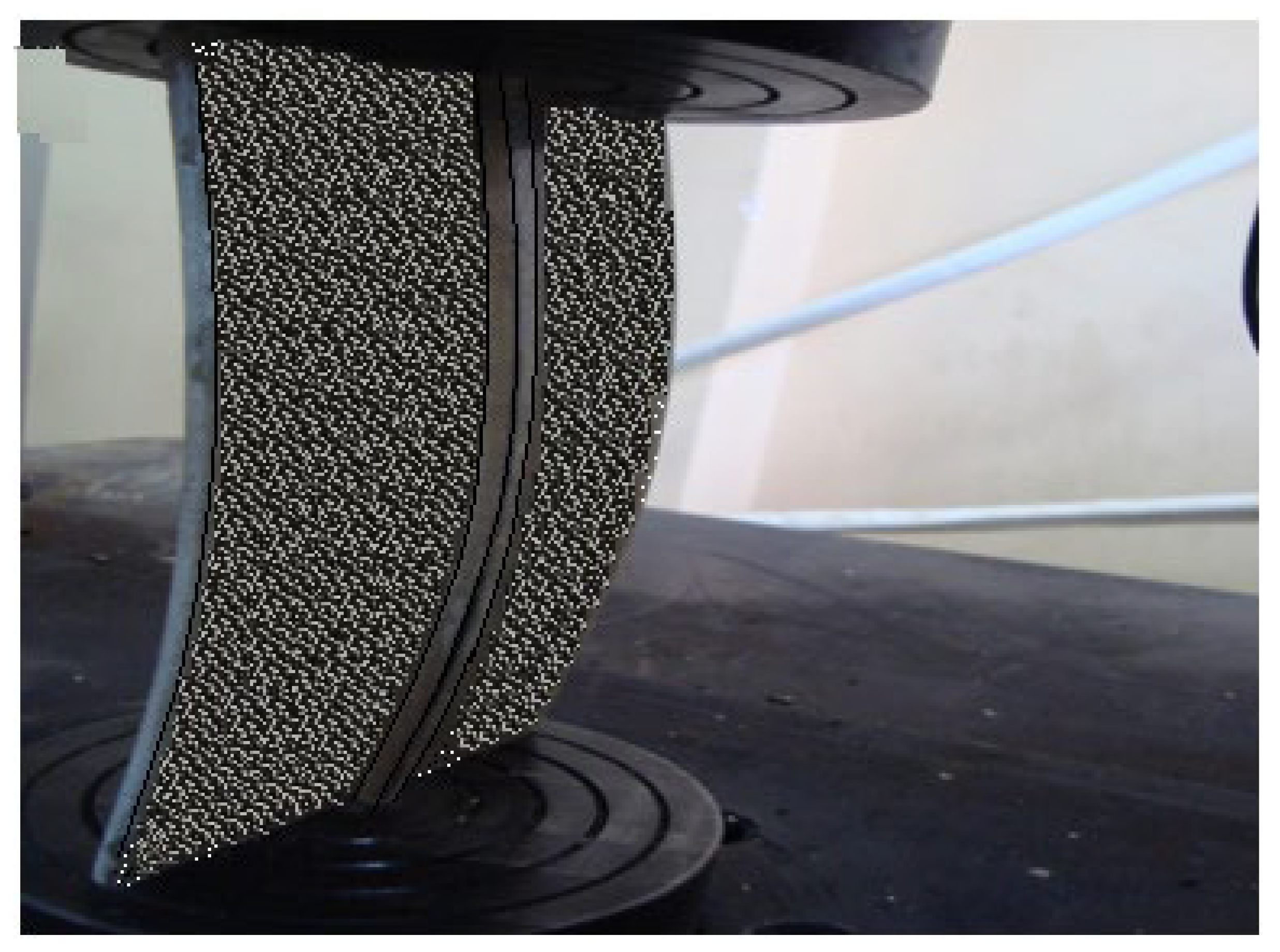
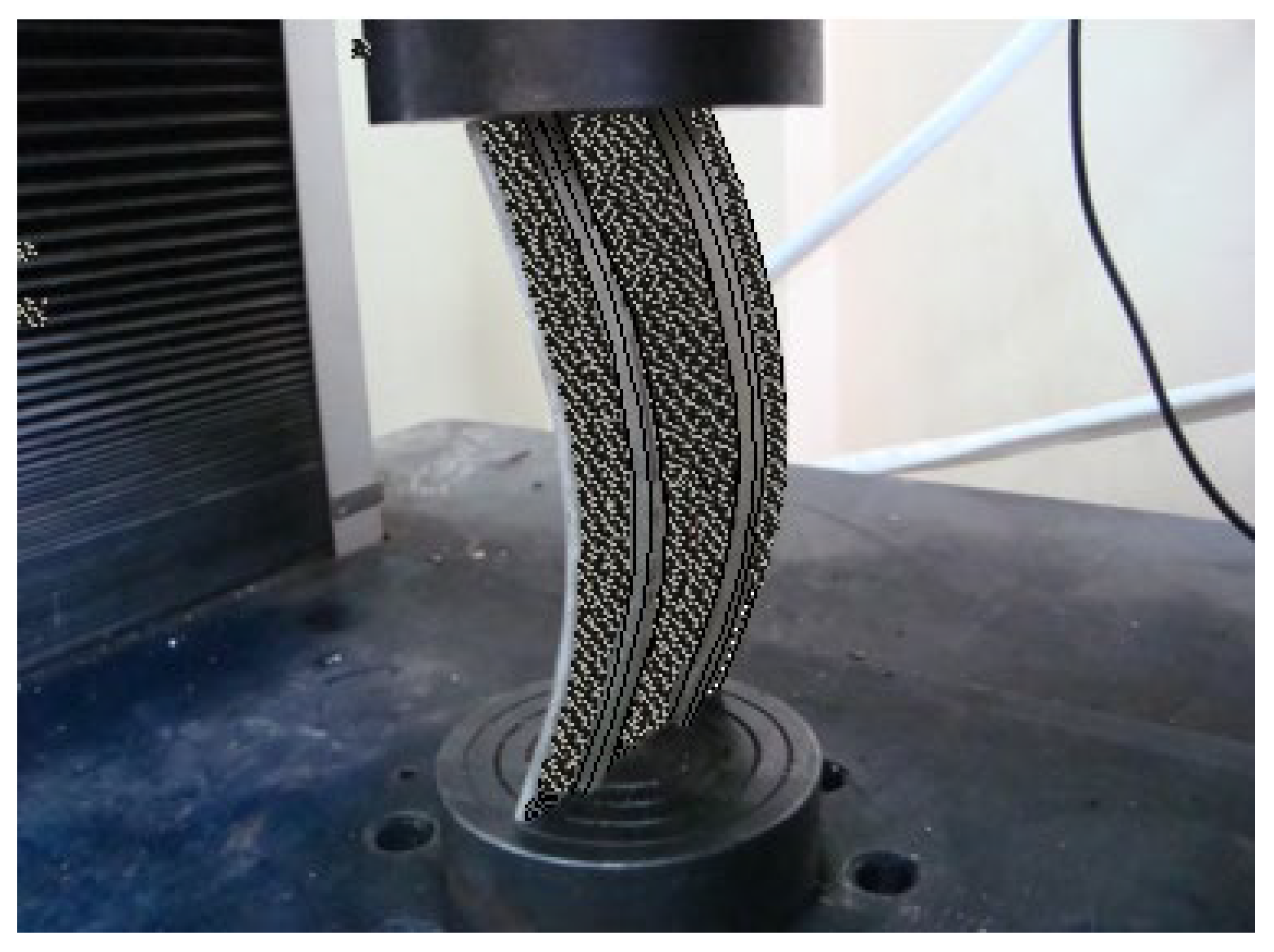
The Lagrange coefficients of the stiffness matrix due to δ u o , δ v o , δ w o , δ Ø x and δ Ø y for stiffener are as in below:
L 11 = A 11 2 x 2 ,   L 12 = 0 ,   L 13 = D 11 c 1 3 x 3 ,   L 14 =   B 11 2 x 2   c 1 D 11 2 x 2 L 22 =   A 22 2 y 2 ,   L 23 = c 1 D 22 3 y 3 ,   L 24 = 0 ,   L 25 = ( B 22   c 1 D 22 ) 2 y 2 L 33 = ( A 55 2 c 2 B 55   c 2 2 C 55 +   N xx ) 2 x 2 + ( A 44 2 c 2 B 44 +   c 2 2 C 44 +   N yy ) 2 y 2 c 1 2 H 11 4 x 4 c 1 2 H 22 4 y 4 L 34 = ( A 55 2 c 2 B 55 + c 2 2 C 55 ) x + ( c 1 E 11 c 1 2 H 11 ) 3 x 3 L 35 = ( A 44 2 c 2 B 44 + c 2 2 C 44 ) y + ( c 1 E 22 c 1 2 H 22 ) 3 y 3 L 44 = ( D 11 2 c 1 E 11 +   c 1 2 H 11 ) 2 x 2   A 55 + 2 c 2 B 55 c 2 2 C 55 ,   L 45 = 0 L 55 = ( C 22 2 c 1 E 22 +   c 1 2 H 22 )   2 y 2   A 44 + 2 c 2 B 44   c 2 2 C 44  
where: C 22 =   A 22 z 2 ,   C 44 =   B 44 z 2 ,   C 55 =   B 55 z 2 .

5. Experiment Setup

The plate with a length of (200 mm), width (100 mm) and thickness (4 mm) is manufactured to be the main plate. The width and depth for the stiffeners are (6 mm) and (4 mm), respectively. The orientation angle for the stiffener is special orthotropic, while the orientation angle of the main plate is cross ply. The dimension in ASTM E1876 is used to manufacture the specimen used in the buckling test [10]. An axial compression machine is used in the buckling test in which the vertical load is (200 KN), as shown in Figure 3.
The speed of the axial compression machine is constant (5 mm/min), in which the specimen is compressed slowly until buckling occurs. A simply supported boundary condition is considered from both sides through the axial compression, while the other two sides are assumed to be free. The buckling test for the un-stiffened plate, plates with one and stiffeners are shown in Figure 4, Figure 5 and Figure 6.
The specimen is inserted into the middle of two circular stiff heads while the upper head is moved slowly towards the fixed lower head using a hydraulic servomotor cylinder. The sensor of the strain gauge is inserted through the plate thickness in the z-direction, in which the strain gauge is connected to a strain meter device. The voltage of the deflection is caught by the strain meter device due to compression axial load. The interface between the buckling machine and the strain meter is calculated to track the deflection. The values of the deflection were saved in a spreadsheet file using Microsoft excel and after the data were treated using a MatLab program.
The deflection through the z-direction is determined as shown below:
δ zz =   ε zz     h
Southwell scheme is a histogram between the compression axial load and the deflection [11]. The compression axial load is easy to read from the screen of the test buckling machine, which has the values (100 N, 150 N, 200 N, 250 N, 300 N, 350 N, 400 N, 450 N, and 500 N). A Southwell plot is a straight line between the bending deflection and in-plane compression mechanical load, in which the slope reflects the critical buckling load. The Southwell plot is shown in Figure 7 for the un-stiffened plate and the plate with one and two stiffeners.

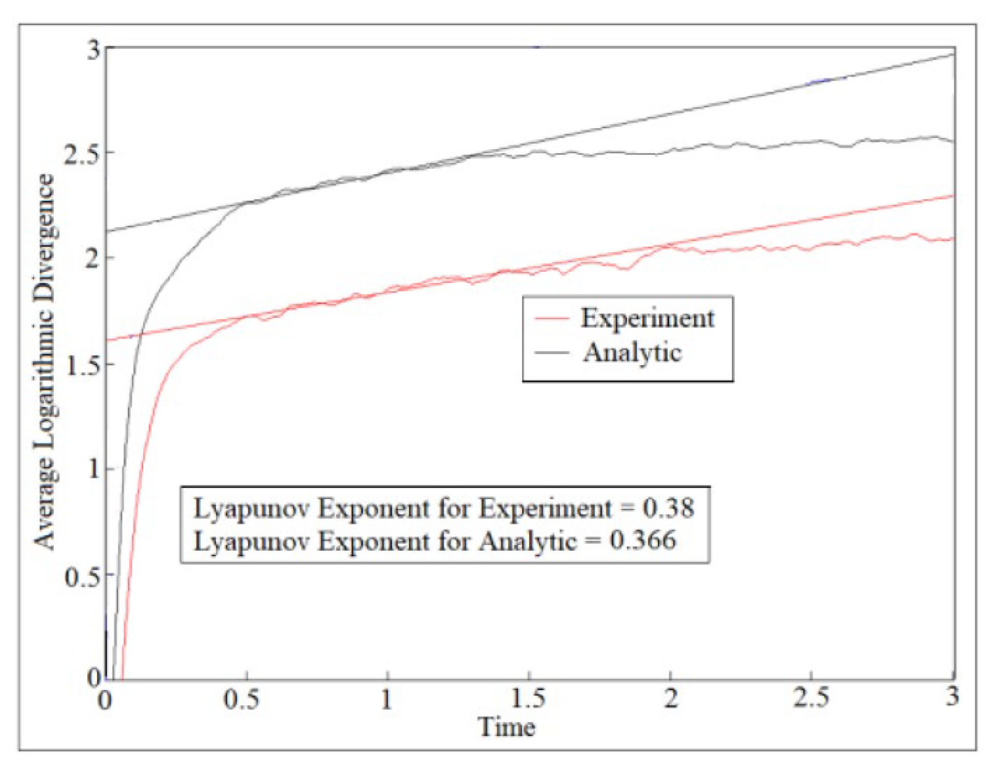
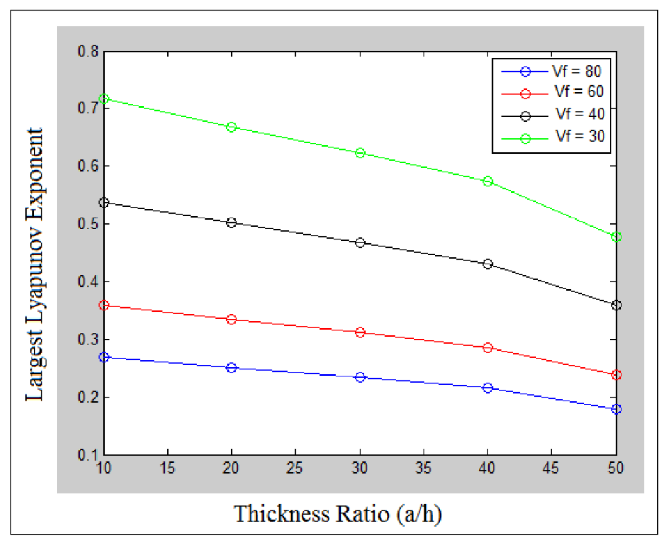
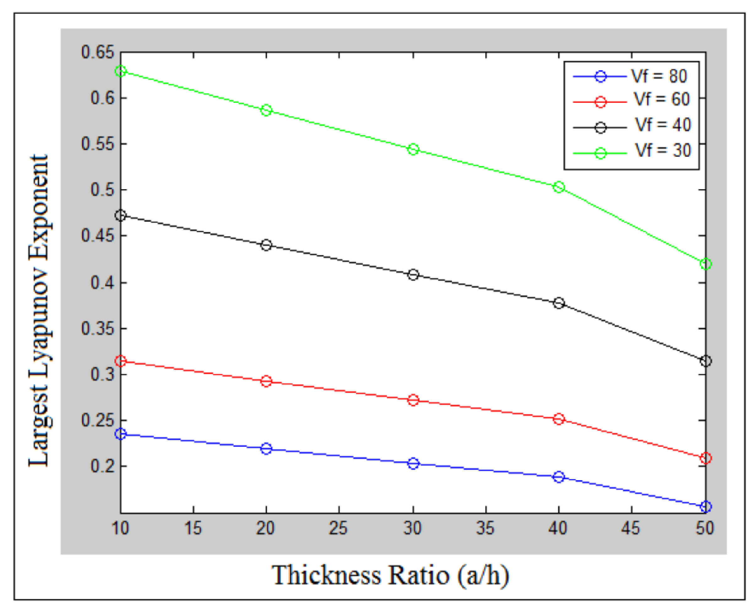
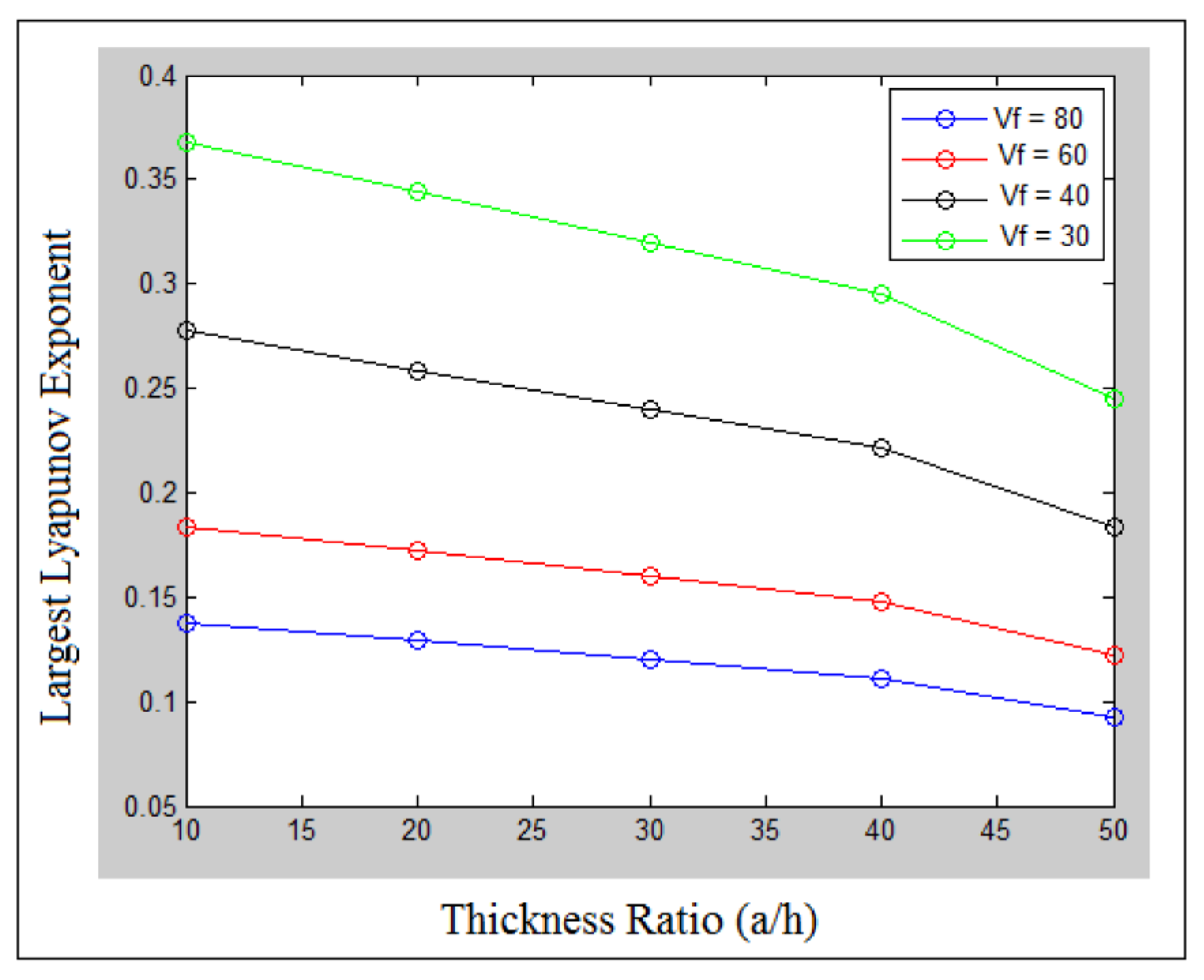
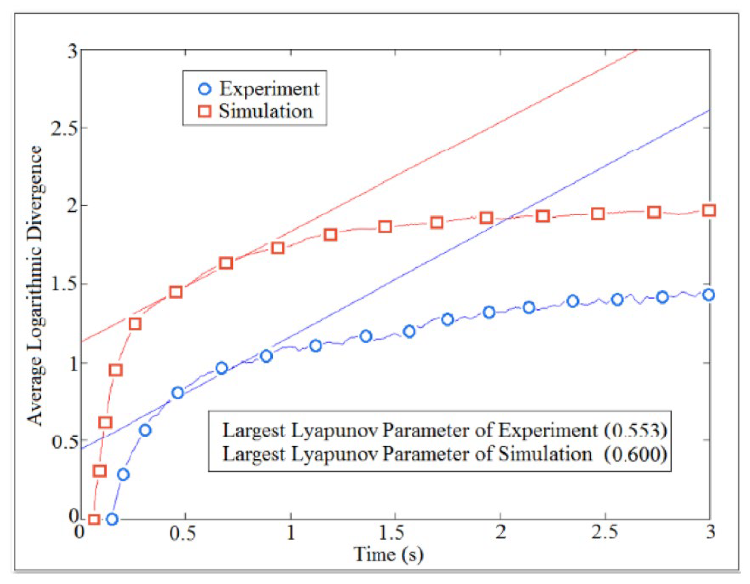
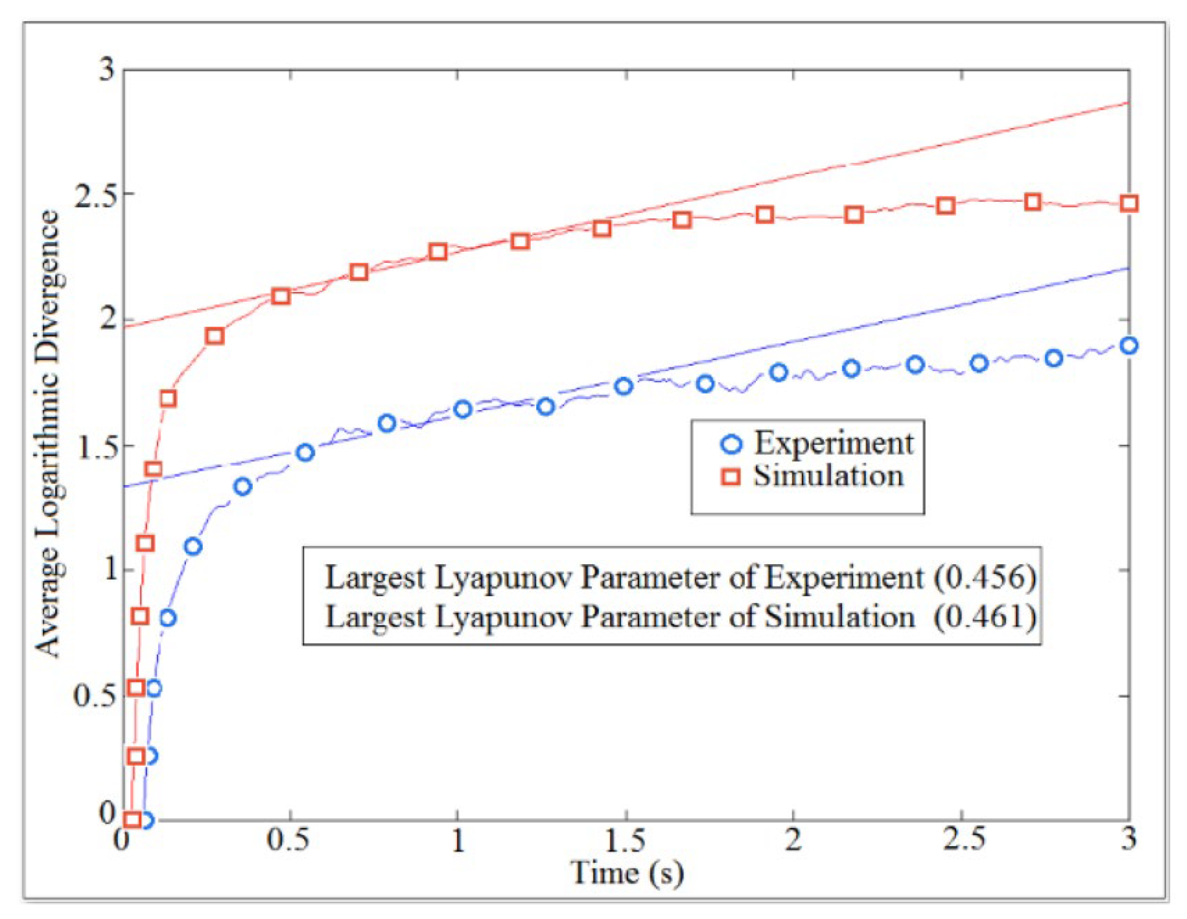
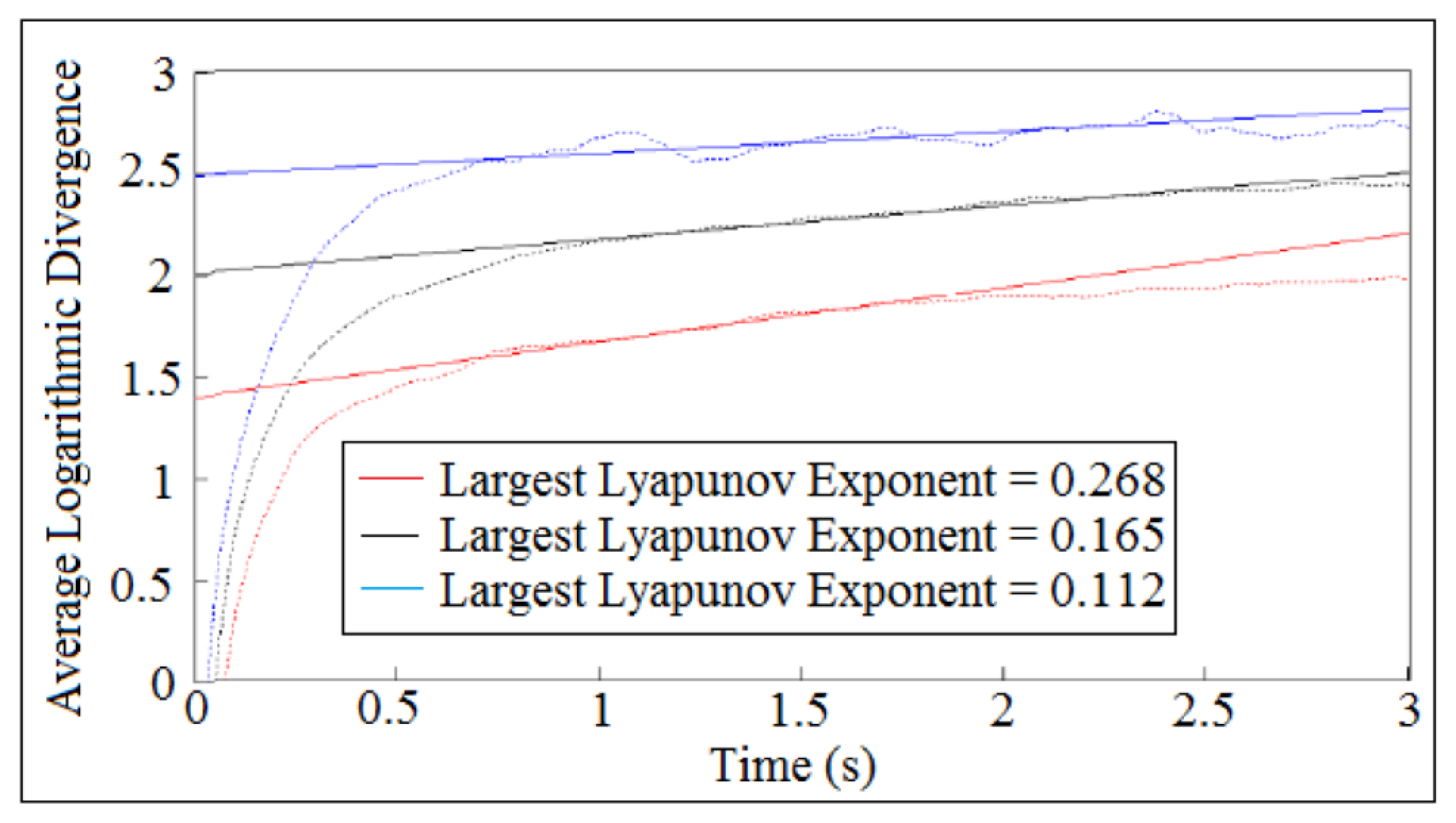
6. Largest Lyapunov Exponent Parameter

The largest Lyapunov exponent is an indicator to chaotic motion. When the Lyapunov parameter of the deflection is above zero it means that the motion of the stiffened plate is chaotic. The Wolf algorithm code based on the average logarithmic divergence is used to extract the values of the largest Lyapunov exponent parameter. The straight line represents the curve fitting of the logarithmic function of the bending deflection which reflects the value of the Lyapunov exponent parameter. The nonlinear curve in an average logarithmic divergence diagram represents the logarithm function of the bending deflection. Equations (13) and (14) are used to build the Wolf algorithm code of the dynamic tool [12]:
d ( t ) =   D     e λ t
y ( i ) = 1 Δ t [ lnd j ( i ) ]
The values of the time delay and embedding dimensions reveal [13,14] the average logarithmic divergence code. Figure 8 shows the comparison of the average logarithmic divergence of bending deflection against time due to critical buckling load at fiber volume fraction (80%) and aspect ratio (2.5). The analytic value of the largest Lyapunov exponent of the bending deflection is calculated using the higher order shear deformation of plates theory. The value of the deflection is tracked experimentally through the z-direction using a strain meter device. The state space of Eigen value problem is used to calculate the bending deflection analytically against time, using the higher order shear deformation theory in the presence of boundary conditions with the aid of MatLab software. The dataset of the bending deflection against time is used in the algorithm code of the average logarithmic divergence to extract the value of the largest Lyapunov exponent parameter.

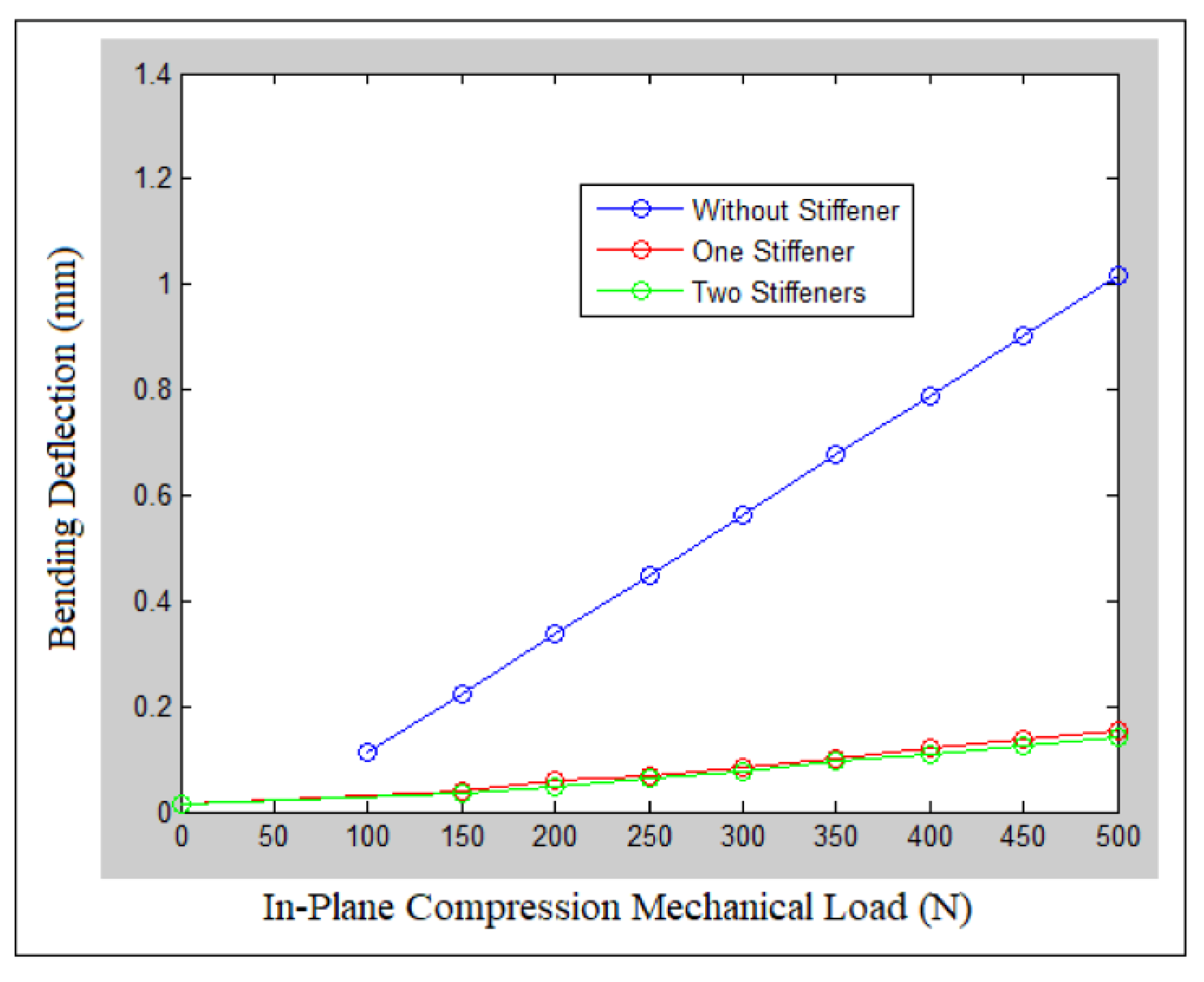
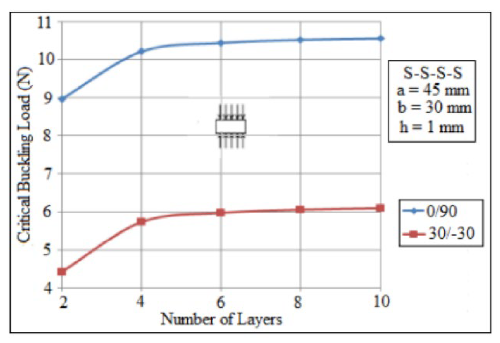
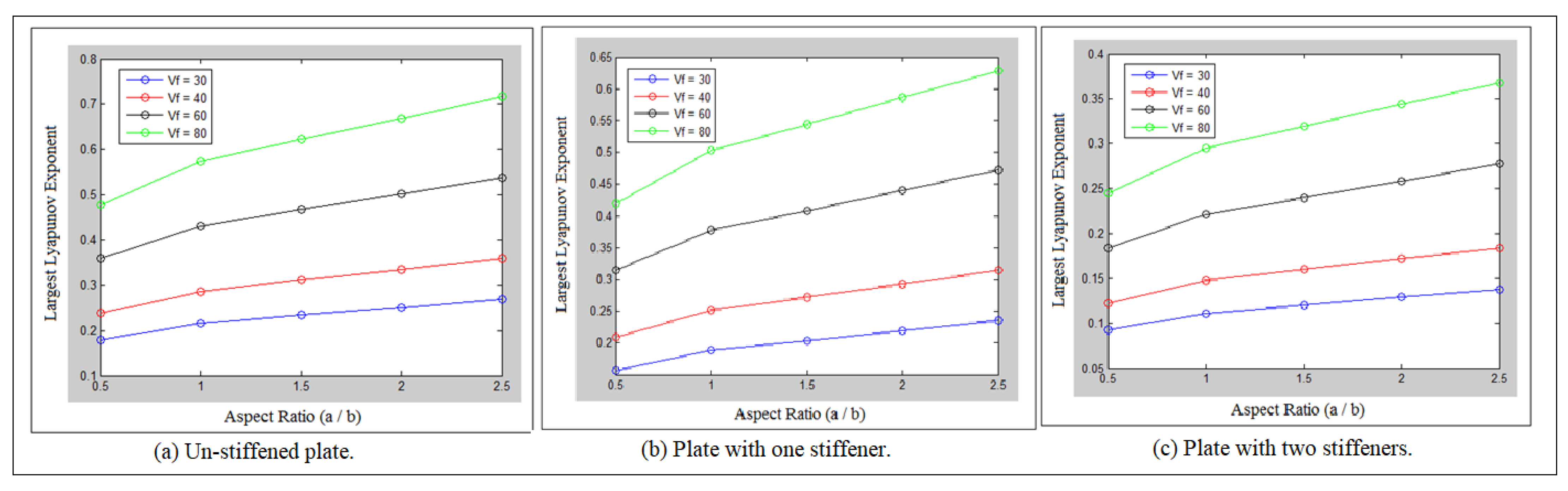
7. Results and Discussions

Figure 9 shows the Lyapunov parameter against the thickness ratio for the un-stiffened plate at different fiber volume fractions. The Lyapunov parameter value declined with the increase in thickness ratio, in which the nonlinear dynamics of the carbon fiber reinforced epoxy composite laminated plate is decreased with the increase in thickness ratio. The value of the largest Lyapunov exponent decreased with the increase in fiber volume fractions. One column of the bending deflection through the plate thickness is used in the average logarithmic divergence approach to quantify the value of the largest Lyapunov exponent. All Lyapunov parameters are above zero, reflecting the chaos motion for the un-stiffened plate.
Figure 10 and Figure 11 show the largest Lyapunov exponent against the thickness ratio at different fiber volume fractions for the plate with one and two stiffeners, in which the stiffeners distribute along the x-axis to reduce the nonlinear dynamics phenomenon in the stiffened composite laminate plate due to critical buckling load. The value of the largest Lyapunov exponent decreased with the increase in fiber volume fractions for the plates with one and two stiffeners while the value of the largest Lyapunov exponent decreased with the increase in the number of stiffeners. Based on the values of the plate dimensions, thickness ratio, number of stiffeners, all the values of the largest Lyapunov exponent are positive, indicating the chaotic motion of the bending deflection.
Figure 12 shows the comparison of the logarithmic function of the bending deflection against time for the plate with one stiffener at a thickness ratio of (20) and a fiber volume fraction of (30%). Experimentally, the bending deflection is calculated along the plate thickness using a strain gauge through a strain meter. Analytically, the bending deflection is determined using the higher order shear deformation theory. Moreover, Figure 13 shows the comparison of the Lyapunov exponent against time for the un-stiffened plate at a thickness ratio of (30) and a fiber volume fraction of (40%). In both figures, the average logarithmic divergence approach is used to calculate the largest Lyapunov exponent parameter. The nonlinear curve of the average logarithmic divergence approach represents the logarithmic value of the bending deflection, while the straight line indicates the Least Squares Curve Fitting of the logarithmic function of the bending deflection.
Figure 14 shows the critical buckling load against the number of layers for the simply supported carbon fiber reinforced epoxy composite laminated plate. The fiber stacking sequence orientation of anti-symmetric cross and angle plies are considered in the simulation. The values of the critical buckling load increased with the increase in the number of layers for both anti-symmetric cross and angle plies. The critical buckling load in both cases settled down at the number of layers (6). The value of the critical buckling load for the anti-symmetric cross ply is higher than the value of the critical buckling load for the anti-symmetric angle ply.
Table 1 shows the comparison of the critical buckling load at different boundary conditions for an anti-symmetric cross laminated plate. The increment of the clamped edges increases the critical buckling load, while the critical buckling load is decreased with the increase in the number of free edges. The thickness ratio for all systems is equal to (50).
Figure 15 shows the logarithmic function of the bending deflection against time for the un-stiffened plate, plate with one and two stiffeners. The un-stiffened plate with a thickness ratio of (20) and a fiber volume fraction of (80%) and the plate with one stiffener at a thickness ratio of (45) and a fiber volume fraction of (80%) are selected, respectively, to quantify the value of the largest Lyapunov exponent. The system with a thickness ratio of (45) and a fiber volume fraction of (80%) is selected to quantify the largest Lyapunov exponent for the plate with two stiffeners.
Figure 16 shows the largest Lyapunov exponent against the aspect ratios for the un-stiffened plate and the plate with one and two stiffeners at different fiber volume fractions for E-glass and polyester resin. The nonlinear dynamic behavior of the bending deflection increased with the increase in aspect ratios and fiber volume fractions. All the values of the largest Lyapunov exponent are positive and above zero, which means that the motion of the bending deflection is non-periodic. The nonlinear dynamic phenomena is decreased with the use of beam stiffeners. The system with an aspect ratio of (2.5) and a fiber volume fraction of ( υ f = 80 % ) for the un-stiffened plate is more chaotic than the other systems, as indicated in Figure 16a. The nonlinear dynamic phenomena is very low for the system with an aspect ratio of (2.5) and a fiber volume fraction of ( υ f = 80 % ) after using the plate with two stiffeners, as shown in Figure 16b. The ANSYS program was used to calculate the bending deflection.

8. Conclusions

This paper discusses the nonlinear dynamics phenomenon of a carbon fiber epoxy composite laminated plate in the presence of stiffeners. All the values of the largest Lyapunov exponent are positive and decrease with the increase in the thickness ratio, while they decrease with the increase in fiber volume fractions. One and two stiffeners are used to decrease the nonlinear dynamics phenomena in the composite laminated plate, since the largest Lyapunov exponent value is decreased. The critical buckling load increased with the increase in the number of clamped edges, since the shear force increases the bending deflection, while the critical buckling load decreases with the increase in the number of free edges, since there is no shear force.

Funding

This research received no external funding.

Institutional Review Board Statement

Not applicable.

Informed Consent Statement

Not applicable.

Data Availability Statement

Not applicable.

Acknowledgments

I want to thank my colleague at the Department of Mechanical Engineering at the University of Baghdad.

Conflicts of Interest

The author declares there is no conflict of interest.

Nomenclatures

aLength of the large span of the rectangular plate, m
bLength of the small span of the rectangular plate, m
hThickness of the un-stiffened composite laminated plate, m
uo, vo, woDisplacement components in the 3-D coordinate system
QijReduced stiffness elements, N/m2
woMid plane deflection along the z-direction, m
tx, hx, bxThickness, depth, distance between stiffeners when the stiffener is placed along the x-axis, mm
ty, hy, byThickness, depth, distance between stiffeners when the stiffener is placed along the y-axis, mm
εzzthe experiment strain through the composite plate thickness
δzzthe experiment bending deflection through the composite plate thickness
λThe largest Lyapunov exponent parameter

References

  1. Lal, A.; Parghi, A.; Markad, K. Post-buckling nonlinear analysis of sandwich laminated composite plate. J. Mater. Today Proc. 2021, 44, 4934–4939. [Google Scholar] [CrossRef]
  2. Yousuf, L.S. Nonlinear dynamics investigation of flexural stiffness of composite laminated plate under the effect of temperature and combined loading using Lyapunov exponent parameter. Compos. Part B Eng. 2021, 219, 108926. [Google Scholar] [CrossRef]
  3. Mondal, S.; Ramachandra, L.S. Nonlinear dynamic pulse buckling of imperfect laminated plate with delamination. Int. J. Solids Struct. 2020, 198, 170–182. [Google Scholar] [CrossRef]
  4. Keshav, V.; Patel, S.N. Non-linear dynamic pulse buckling of laminated composite curved panels. Int. J. Struct. Eng. Mech. 2020, 73, 181–190. [Google Scholar]
  5. Keshav, V.; Patel, S.; Kumar, R. Nonlinear dynamic buckling and failure study of laminated composite plates subjected to axial impulse loads. In Advances in Fluid Mechanics and Solid Mechanics; Springer: Berlin/Heidelberg, Germany, 2020; pp. 281–295. [Google Scholar]
  6. Balkan, D.; Demir, Ö.; Arıkoğlu, A. Dynamic analysis of a stiffened composite plate under blast load: A new model and experimental validation. Int. J. Impact 2020, 143, 103591. [Google Scholar] [CrossRef]
  7. Yousyf, L.S. Nonlinear Dynamics Suppression of Bending Deflection in a Composite Laminated Plate Using a Beam Stiffener Due to Critical Buckling Load and Shear Force. J. Appl. Sci. 2022, 12, 1204. [Google Scholar] [CrossRef]
  8. Reddy, J.N. Mechanics of Laminated Composite Plates and Shells: Theory and Analysis; CRC press: Boca Raton, FL, USA, 2003. [Google Scholar]
  9. Troitsky, M.; Hoppmann, W. Stiffened plates: Bending, stability and vibrations. J. Appl. Mech. 1977, 44, 516. [Google Scholar] [CrossRef]
  10. Gopalan, V.; Suthenthiraveerappa, V.; David, J.S.; Subramanian, J.; Annamalai, A.R.; Jen, C.-P. Experimental and numerical analyses on the buckling characteristics of woven flax/epoxy laminated composite plate under axial compression. Polymers 2021, 13, 995. [Google Scholar] [CrossRef] [PubMed]
  11. Sun, C.-T.; Adnan, A. Mechanics of Aircraft Structures; John Wiley & Sons: Hoboken, NJ, USA, 2021. [Google Scholar]
  12. Terrier, P.; Reynard, F. Maximum lyapunov exponent revisited: Long-term attractor divergence of gait dynamics is highly sensitive to the noise structure of stride intervals. Gait Posture 2018, 66, 236–241. [Google Scholar] [CrossRef] [PubMed]
  13. Hussain, V.S.; Spano, M.L.; Lockhart, T.E. Effect of data length on time delay and embedding dimension for calculating the lyapunov exponent in walking. J. R. Soc. Interface 2020, 17, 20200311. [Google Scholar] [CrossRef] [PubMed]
  14. Matilla-García, M.; Morales, I.; Rodríguez, J.M.; Marín, M.R. Selection of embedding dimension and delay time in phase space reconstruction via symbolic dynamics. Entropy 2021, 23, 221. [Google Scholar] [CrossRef]
Figure 1. Loading and boundary condition of rectangular plate.
Mathematics 10 02020 g001
Figure 2. Stiffened plate with different stiffeners along x and y directions.
Mathematics 10 02020 g002
Figure 3. Buckling test machine.
Mathematics 10 02020 g003
Figure 4. Rectangular plate without stiffeners.
Mathematics 10 02020 g004
Figure 5. Rectangular plate with one stiffener.
Mathematics 10 02020 g005
Figure 6. Rectangular plate with two stiffeners.
Mathematics 10 02020 g006
Figure 7. Buckling deflection.
Mathematics 10 02020 g007
Figure 8. Comparison of Lyapunov exponent parameter.
Mathematics 10 02020 g008
Figure 9. Largest Lyapunov exponent against thickness ratio for un-stiffened plate.
Mathematics 10 02020 g009
Figure 10. Largest Lyapunov exponent against thickness ratio for plate with one stiffener.
Mathematics 10 02020 g010
Figure 11. Largest Lyapunov exponent against thickness ratio for plate with two stiffeners.
Mathematics 10 02020 g011
Figure 12. Largest Lyapunov exponent against time for plate with one stiffener.
Mathematics 10 02020 g012
Figure 13. Largest Lyapunov exponent against time for un-stiffened plate.
Mathematics 10 02020 g013
Figure 14. Critical buckling load against number of layers.
Mathematics 10 02020 g014
Figure 15. Largest Lyapunov exponent against time for un-stiffened plate, and plate with one and two stiffeners.
Mathematics 10 02020 g015
Figure 16. Largest Lyapunov exponent for unstiffened plate and plate with one and two stiffeners.
Mathematics 10 02020 g016
Table 1. Comparison of critical buckling load for different boundary conditions.
Boundary ConditionsAnalytic (N)Numerical (N)Error (%)
S-F-S-F16.42617.5336.317
S-F-S-S17.02318.1156.032
S-F-S-C19.38920.4685.272
S-S-S-S35.23236.3513.078
S-S-S-C59.28860.4091.855
Publisher’s Note: MDPI stays neutral with regard to jurisdictional claims in published maps and institutional affiliations.

