Article

Numerical Stability and Performance of Semi-Explicit and Semi-Implicit Predictor–Corrector Methods

1
Ecole Polytechnique de Louvain, Université Catholique de Louvain, 1348 Louvain-la-Neuve, Belgium
2
Department of Computer-Aided Design, Saint Petersburg Electrotechnical University “LETI”, 197376 Saint Petersburg, Russia
3
Youth Research Institute, Saint Petersburg Electrotechnical University “LETI”, 197376 Saint Petersburg, Russia
4
Institute of Mechanics, Materials and Civil Engineering (IMMC), Université Catholique de Louvain, L4.05.02, 1348 Louvain-la-Neuve, Belgium
*
Author to whom correspondence should be addressed.
Mathematics 2022, 10(12), 2015; https://doi.org/10.3390/math10122015
Submission received: 21 May 2022 / Accepted: 9 June 2022 / Published: 11 June 2022
(This article belongs to the Section Computational and Applied Mathematics)

Abstract

:
Semi-implicit multistep methods are an efficient tool for solving large-scale ODE systems. This recently emerged technique is based on modified Adams–Bashforth–Moulton (ABM) methods. In this paper, we introduce new semi-explicit and semi-implicit predictor–corrector methods based on the backward differentiation formula and Adams–Bashforth methods. We provide a thorough study of the numerical stability and performance of new methods and compare their stability with semi-explicit and semi-implicit Adams–Bashforth–Moulton methods and their performance with conventional linear multistep methods: Adams–Bashforth, Adams–Moulton, and BDF. The numerical stability of the investigated methods was assessed by plotting stability regions and their performances were assessed by plotting error versus CPU time plots. The mathematical developments leading to the increase in numerical stability and performance are carefully reported. The obtained results show the potential superiority of semi-explicit and semi-implicit methods over conventional linear multistep algorithms.

1. Introduction

Using systems of ordinary differential equations (ODE) is a common approach for describing dynamical systems. It is a natural way of expressing the evolution of a system whether it is a mechanical [1], electrical [2], chemical [3], or biological system [4], etc. From a more contemporary perspective, the solution of ODEs is proving crucial in modeling epidemics [5]. Simulating dynamical systems on discrete computers requires the discretization of ODEs, which is usually performed by numerical integration methods [6]. The requirements for numerical methods increase with the rapid growth of complexity and stiffness of the simulated systems. Therefore, the development of new computationally efficient and stable numerical methods is of certain interest. One of the main classes of ODE solvers are linear multistep methods which efficiently solve ODE systems using a single evaluation of the right-hand function at each integration step. Within this family, some methods are implicit, such as the backward differentiation formula (BDF) or the Adams–Moulton method, while others are explicit, such as the Adams–Bashforth method, which has been applied to the population dynamics model by H. Jafari et al. [7]. Implicit methods possess better numerical stability than the explicit ones but require performing Newton’s method iterations on each step and are therefore more computationally expensive [8]. Moreover, explicit methods require smaller step sizes and may lose the order of accuracy in some cases such as stiff equations [9,10]. On the other hand, there are also explicit Runge–Kutta methods which require more function evaluations, and implicit Runge–Kutta methods which are A-stable but require greater computational effort than the linear multistep methods due to a bigger system to solve. However, Hairer et al. showed in [6] that an explicit Runge–Kutta method can be faster than a multistep method. Moreover, some Runge–Kutta methods are designed to be efficient such as SIRK and DIRK methods [11], but Runge–Kutta methods have another advantage: they are parallelizable [12,13]. On top of that, a predictor–corrector method, Adams–Bashforth–Moulton (ABM), was proposed as a compromise between explicit and implicit linear multistep methods. The idea is to predict the integration step by Adams–Bashforth and correct it with Adams–Moulton. Thus, computations are entirely explicit and this technique has better numerical stability than Adams–Bashforth [14]. Recently, efficient semi-explicit and semi-implicit modifications of the ABM have been proposed in [15] as a trade-off between the efficiency of explicit methods and the accuracy of the implicit ones.
In this paper, we develop the mathematical expressions needed to investigate the numerical stability of semi-explicit and semi-implicit ABM and BDF (PEC) methods in Section 2. In Section 3, we use the mathematical developments to plot the stability regions of the two methods. Finally, a discussion of the obtained results is given in the last section.

2. Materials and Methods

Semi-explicit and semi-implicit modifications of the ABM methods were developed to gain computational efficiency and numerical stability. First, the semi-explicit modification aims to keep the computational efficiency of the explicit scheme while extending its numerical stability [16]. For the semi-implicit modification, the goal is to keep good numerical stability while reducing the computational cost. Indeed, a fully implicit scheme requires solving at each step a large-scale system for each variable while the semi-implicit modification will solve each equation separately for one variable at a time.
Let us consider the semi-explicit and semi-implicit modifications of the predictor–corrector Adams–Bashforth–Moulton formula as described in [15]. In this section, we use the same methodology as in [17]. In the original ABM integration, all calculations are explicit. Furthermore, the stability of such an integration technique is higher than that of the explicit Adams–Bashforth method [15]. Note that all abbreviations are listed at the end of the article.

2.1. Semi-Explicit and Semi-Implicit ABM Methods

Following [17], we apply the two methods on a sample ODE system:
x ˙   =   f ( x , y , t ) y ˙   =   g ( x , y , t )
The way that these equations are treated defines the unique properties of these methods: decreasing computations costs while attaining greater numerical stability.
The semi-explicit and semi-implicit methods are predictor–corrector methods (like the initial ABM method) and their predictor stage is computed with the Adams–Bashforth method:
x n + 1 p =   x n + h i = 1 k B i f ( x n i , y n i , t n i ) y n + 1 p =   y n + h i = 1 k B i g ( x n i , y n i , t n i ) ,
where B i are the coefficients of the Adams–Bashforth method. For the corrector stage, we use the predicted value and the values obtained during this step to obtain the solution.

2.1.1. General Description of Semi-Explicit and Semi-Implicit BDF (PEC) Methods

Well-known backward differentiation formula (BDF) is a family of A ( α ) -stable linear multistep methods. Using this formula as a corrector allows increasing the stability of the resulting method. The equation of the corrector stage in the semi-explicit variant of the BDF-predictor–corrector (BDF PEC) method reads:
x n + 1   +   i = 1 k α i x n + 1 i =   β 0 f ( x n + 1 p , y n + 1 p , t n + 1 ) y n + 1   +   i = 1 k α i y n + 1 i =   β 0 g ( x n + 1 , y n + 1 p , t n + 1 ) ,
where α i and β 0 are coefficients of the BDF method.
Backward differentiation formula can be transformed into a semi-implicit variant of the BDF (PEC) method. Then, the BDF (PEC) semi-implicit corrector formula reads:
x n + 1   +   i = 1 k α i x n + 1 i =   β 0 f ( x n + 1 , y n + 1 p , t n + 1 ) y n + 1   +   i = 1 k α i y n + 1 i =   β 0 g ( x n + 1 , y n + 1 , t n + 1 ) ,
where α i and β 0 are the coefficients of the BDF method.
In Table 1, we present a set of coefficients for the BDF (PEC) methods.

2.1.2. Semi-Explicit ABM Method

The corrector of the semi-explicit scheme is given by:
x n + 1 =   x n   +   h M 1 f ( x n + 1 p , y n + 1 p , t n + 1 )   +   h i = 1 k M i + 1 f ( x n i , y n i , t n i ) y n + 1 =   y n   +   h M 1 g ( x n + 1 , y n + 1 p , t n + 1 )   +   h i = 1 k M i + 1 g ( x n i , y n i , t n i ) ,
where M i denotes the coefficients of the Adams–Moulton method, k denotes the number of stages, h denotes the integration step, and t denotes the time moment. Note that x p and y p are the predicted values of x and y computed using Equation (2). Observe that all computations are explicit because there is no equation to solve since x n + 1 p , y n + 1 p and x n are known in the first equation of system (5). For the second equation, we use the already obtained and corrected value x n + 1 . Therefore, the considered method is a semi-explicit integrator.

2.1.3. Semi-Implicit ABM Method

On the other hand, the semi-implicit method requires an implicit calculation using Newton’s method for each equation. Its corrector is as follows:
x n + 1 =   x n   +   h M 1 f ( x n + 1 , y n + 1 p , t n + 1 )   +   h i = 1 k M i + 1 f ( x n i , y n i , t n i ) y n + 1 =   y n + h M 1 g x n + 1 , y n + 1 , t n + 1   +   h i = 1 k M i + 1 g ( x n i , y n i , t n i ) .
Note that with this method, one does not need to compute the first predictor stage (in this case x n + 1 p in (2)) which can be an advantage if f is a computationally expensive function. Finally, observe that the method is semi-implicit since all equations must be solved for the associated variable. As in the previous case, the second equation uses the already obtained x n + 1 .

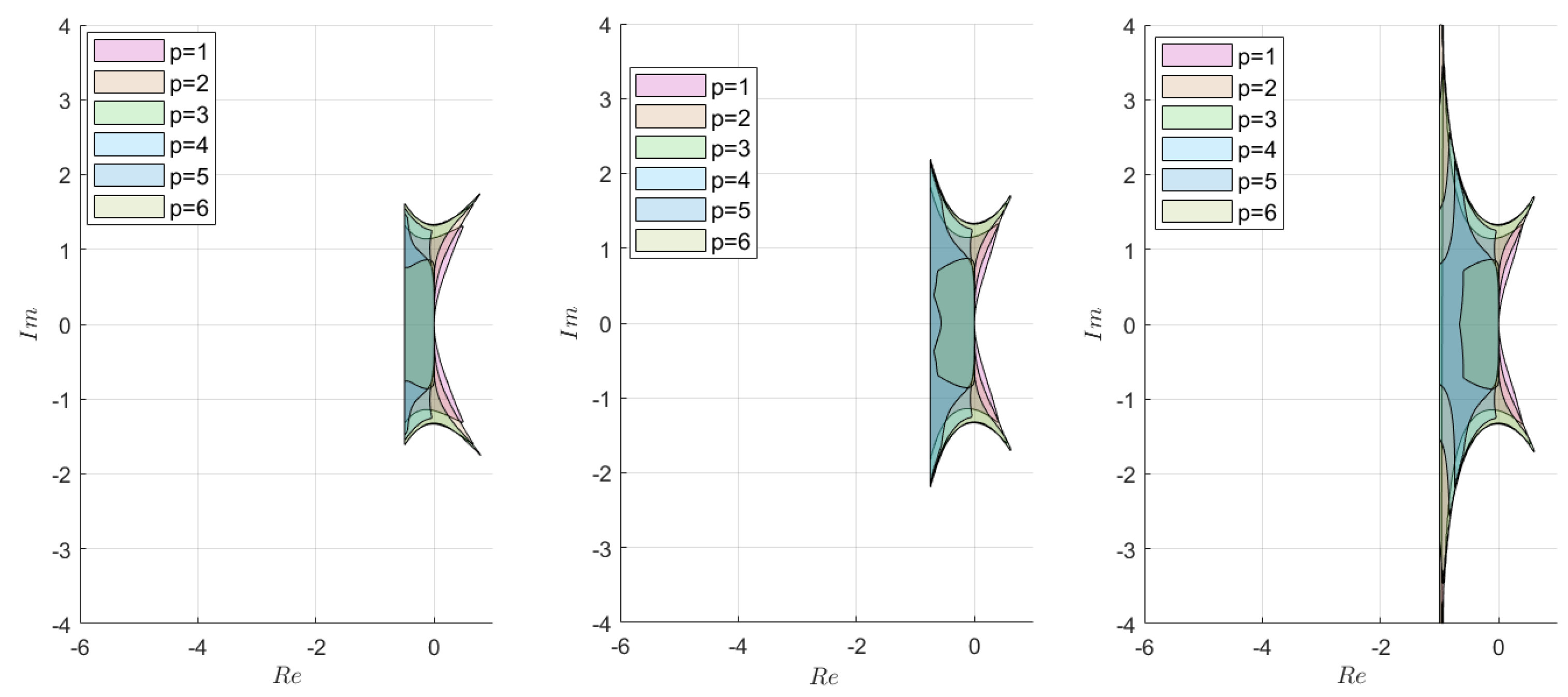
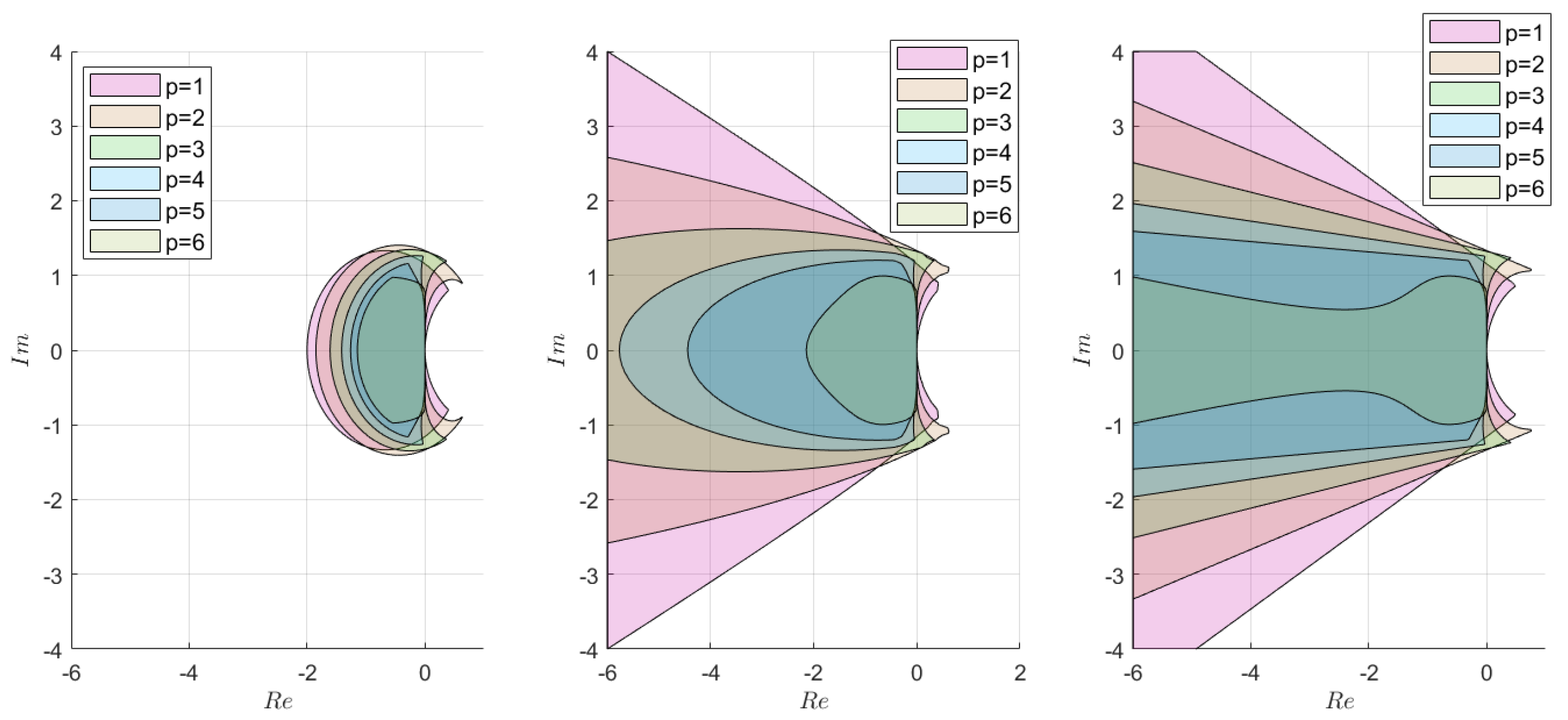
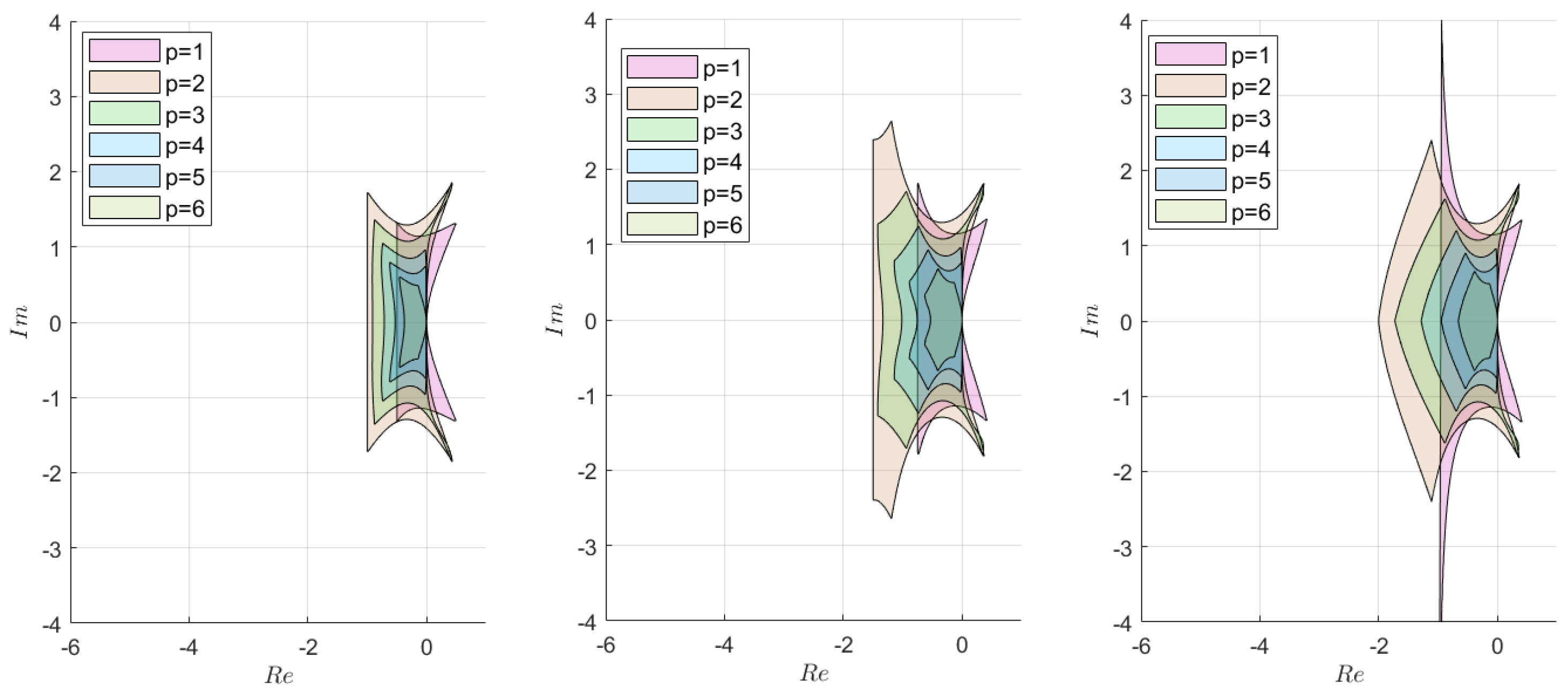
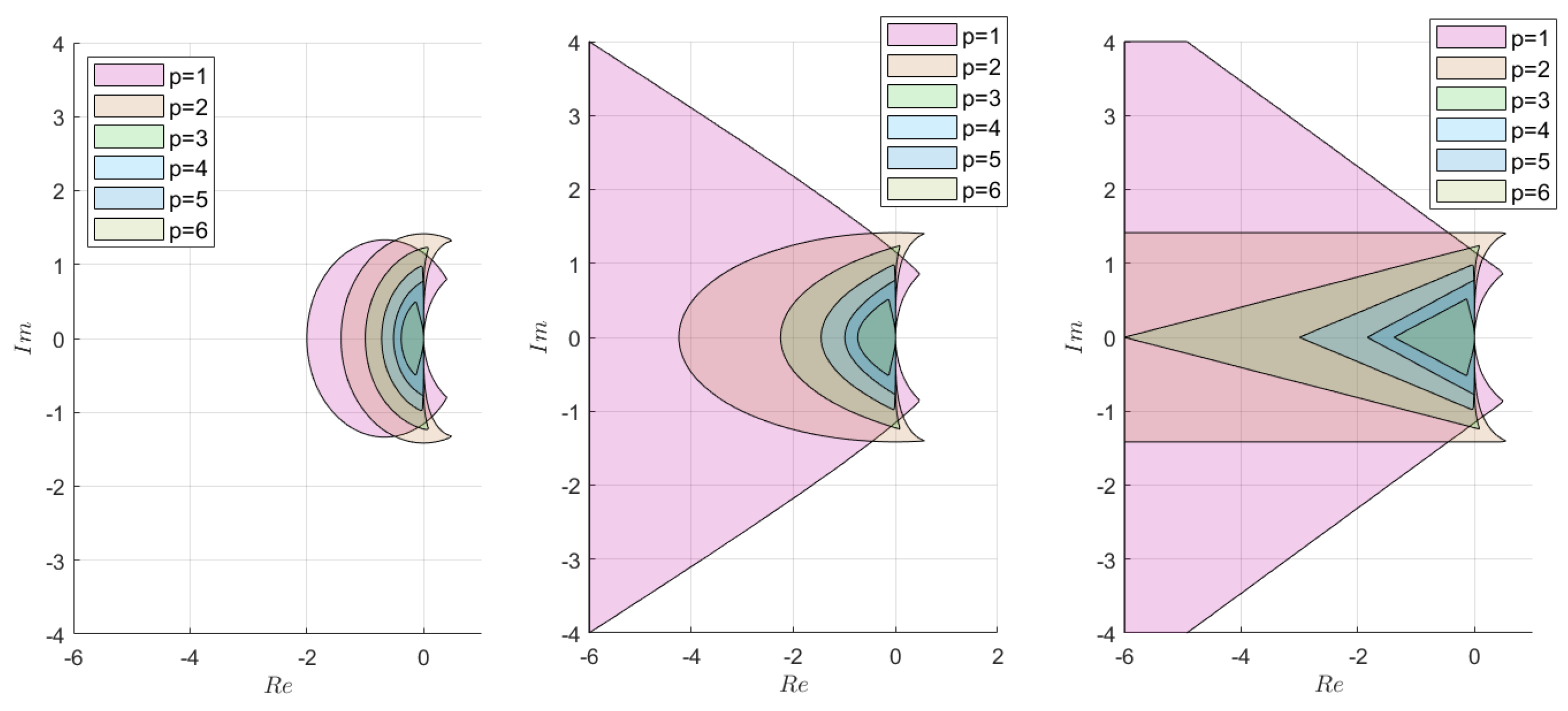
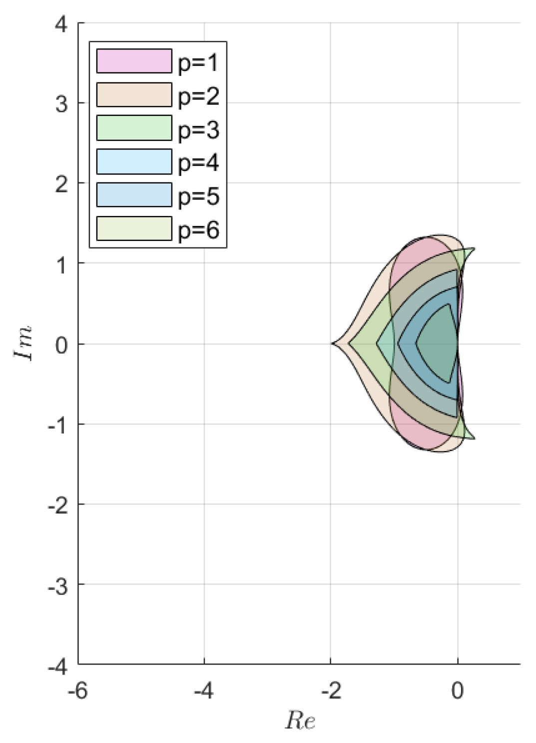
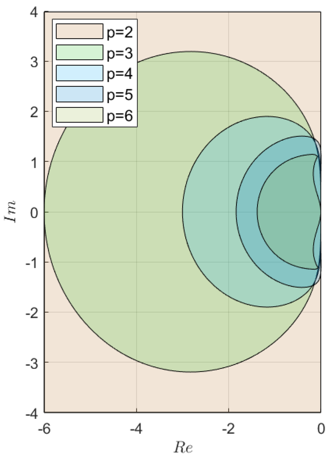
2.2. Stability Analysis

Since semi-explicit methods do not exist for ODEs with less than two dimensions, we cannot use Dahlquist’s first-order test equation. Instead, we choose the similar approach used in [17] that applies a two-dimensional test problem. Let us compose a matrix A of dimension 2   ×   2 for the studied problem:
x ˙   =   A x   =   A 11 A 12 A 21 A 22 x ,
where x   =   x y . We suppose that this matrix A has two conjugate eigenvalues λ 1 , 2   =   σ   ±   j ω .
This subsection aims to form the polynomial matrix characterizing the stability of the methods and extract its eigenvalues. Let us define this matrix as
P ( z )   =   P 11 ( z ) P 12 ( z ) P 21 ( z ) P 22 ( z )
with z as the delay operator.
To begin, one has to study the stability of the predictor which is used in both semi-explicit and semi-implicit ABM methods. We can form the matrix polynomial of the predictor p ( z ) as
p ( z )   =   ( I + B 1 h A ) z p 1   +   B 2 h A z p 2   + + B 6 h A z p 6   =   p 11 ( z ) p 12 ( z ) p 21 ( z ) p 22 ( z )
where I is the identity matrix, h is the integration step and we take the terms with a non-negative power of z according to the order p. Recall that B is the vector of coefficients of the Adams–Bashforth method while M is the vector of coefficients of the Adams–Moulton method, and p denotes the lengths of B and M. In other words, p is the order of the method considered. Formula (9) is common to the stability analysis of both methods.

2.2.1. Semi-Explicit ABM Method

One can rewrite the first equation of system (5) as:
x n + 1   =   1 + M 2 h A 12 M 2 h A 11 x n   +   M 3 h A 11 A 12 x n   + + M 6 h A 11 A 12 x n 4   +   M 1 h A 11 A 12 x n + 1 p
Recall that x   =   x y and x n + 1 p   =   x n + 1 p y n + 1 p . According to order p, we take the terms in which the index of M is not greater than p. This leads to:
P 11 ( z ) =   ( 1 + M 2 h A 11 ) z p 1   +   M 3 h A 11 z p 2   + + M 6 h A 11 z p 5   +   M 1 h ( A 11 p 11 + A 12 p 21 ) P 12 ( z ) =   M 2 h A 12 z p 1   +   M 3 h A 12 z p 2 + + M 6 h A 12 z p 5   +   M 1 h ( A 11 p 12 + A 12 p 22 )
in which we keep the terms with the non-negative power of z. Following the same idea, we can write the second equation of system (5) as follows:
y n + 1   =   M 2 h A 21 1 + M 2 h A 22 x n   +   M 3 h A 21 A 22 x n 1 + + M 6 h A 21 A 22 x n 4   +   M 1 h 0 A 22 x n + 1 p   +   M 1 h A 21 0 x n + 1
Note that, in this equation, we reuse x n + 1 —which we just computed—such that the computation is explicit. From this equation, we obtain matrix P ( z ) of Equation (8) as:
P 21 ( z ) =   M 2 h A 21 z p 1   +   M 3 h A 21 z p 2 + + M 6 h A 21 z p 5   +   M 1 h ( A 21 P 11 + A 22 p 21 ) P 22 ( z ) =   ( 1 + M 2 h A 22 ) z p 1   +   M 3 h A 22 z p 2 + + M 6 h A 22 z p 5   +   M 1 h ( A 21 P 12 + A 22 p 22 )
with P 11 and P 12 already computed.

2.2.2. Semi-Implicit ABM Method

From the first equation of system (6), we can write:
( 1 M 1 h A 11 ) x n + 1   =   1 + M 2 h A 11 M 2 h A 12 x n   +   M 3 h A 11 A 12 x n 1 + + M 6 h A 11 A 12 x n 4   +   M 1 h 0 A 12 x n + 1 p
This leads to the expressions of P 11 ( z ) and P 12 ( z )
P 11 ( z ) =   ( ( 1 + M 2 h A 11 ) z p 1 + M 3 h A 11 z p 2 + + M 6 h A 11 z p 5 + M 1 h A 12 p 21 ) ( 1 M 1 h A 11 ) 1 P 12 ( z ) =   ( M 2 h A 12 z p 1 + M 3 h A 12 z p 2 + + M 6 h A 12 z p 5 + M 1 h A 12 p 22 ) ( 1 M 1 h A 11 ) 1
Following the same idea, we can write the second equation of system (6) as follows:
( 1 M 1 h A 22 ) y n + 1   =   M 2 h A 21 1 + M 2 h A 22 x n   +   M 3 h A 21 A 22 x n 1 + + M 6 h A 21 A 22 x n 4   +   M 1 h A 21 0 x n + 1 p
This leads to the expressions of P 21 ( z ) and P 22 ( z ) :
P 21 ( z ) =   ( M 2 h A 21 z p 1 + M 3 h A 21 z p 2 + + M 6 h A 21 z p 5 + M 1 h A 21 P 11 ( z ) ) ( 1 M 1 h A 22 ) 1 P 22 ( z ) =   ( ( 1 + M 2 h A 22 ) z p 1 + M 3 h A 22 z p 2 + + M 6 h A 22 z p 5 + M 1 h A 21 P 12 ( z ) ) ( 1 M 1 h A 22 ) 1

2.2.3. Semi-Explicit BDF (PEC) Method

Using the same technique, formulas for stability matrices are obtained for the semi-explicit BDF (PEC) method (3):
P 11 ( z ) =   α 1 z p 1   +   α 2 z p 2 + + β 0 h ( A 11 p 11 ( z ) + A 12 p 21 ( z ) ) P 12 ( z ) =   β 0 h ( A 11 p 12 ( z ) + A 12 p 22 ( z ) ) P 21 ( z ) =   β 0 h ( A 21 P 11 ( z )   +   A 22 p 21 ( z ) ) P 22 ( z ) =   α 1 z p 1   +   α 2 z p 2 + + β 0 h ( A 21 P 12 ( z ) + A 22 p 22 ( z ) ) .

2.2.4. Semi-Implicit BDF (PEC) Method

Stability matrices for the semi-implicit BDF (PEC) method (4) read in a similar way:
P 11 ( z ) =   ( α 1 z p 1 + α 2 z p 2 + + β 0 h A 12 p 21 ( z ) ) ( 1 β 0 h A 11 ) 1 P 12 ( z ) =   β 0 h A 12 p 22 ( z ) ( 1 β 0 h A 11 ) 1 P 21 ( z ) =   β 0 h A 21 P 11 ( z ) ( 1 β 0 h A 22 ) 1 P 22 ( z ) =   ( α 1 z p 1 + α 2 z p 2 + + β 0 h A 21 P 12 ( z ) ) ( 1 β 0 h A 22 ) 1 .

2.3. Test Problem for Estimating Method Stability

Following the ideas of [17] and particularly [18] for a two-dimensional problem, matrix A of the test problem is built such that the conjugate eigenvalues λ 1 , 2 defined in Section 2.2 are the eigenvalues of this matrix A. This will allow us to study the same stability regions with values R ( | λ 1 , 2 | ) . Moreover, the matrix A is built such that every possible 2   ×   2 matrix with those two conjugate eigenvalues must be easily derived. In order to obtain such a matrix, we must first ensure that A 12   =   A 21 . Then, all those two-dimensional matrices can be described by a ratio between the first entry of the diagonal and the second one. There exist two extreme cases for such matrices: an asymmetric triangular matrix and the symmetric one with respect to the diagonal elements. Indeed, for 2   ×   2 matrices, we have two diagonal entries such that we can express the first one as a multiple of the second one.
Taking into account those considerations, we obtain the following coefficients of the test matrix for problem (7):
A 11 =   k A 22 A 12 =   λ 2 ( 1 + k ) A 22 λ + k A 22 2 A 21 =   A 12 A 22 =   2 σ 1 + k
where we define k   =   A 11 / A 22 , called the symmetry coefficient. This matrix was developed such that every matrix with conjugate eigenvalues can be expressed by this factor k with the two extreme cases. On the one hand, the coefficient k can be 0 or ∞ for an asymmetric triangular matrix (Frobenius normal form). On the other hand, for a matrix in Jordan normal form, coefficient k is equal to 1. All the other matrices that do not have one of these two forms have an intermediate value of k. The two extreme cases can be viewed as limits for stability functions.
Finally, in order to study the stability regions of the two methods, we need to take the largest eigenvalue of P ( z ) in the modulus. We can do this with the characteristic polynomial of P ( z ) given by ( h λ P 11 ( z ) ) ( h λ P 22 ( z ) ) P 21 ( z ) P 12 ( z ) . These roots must be less than 1 in modulus to make the method stable.

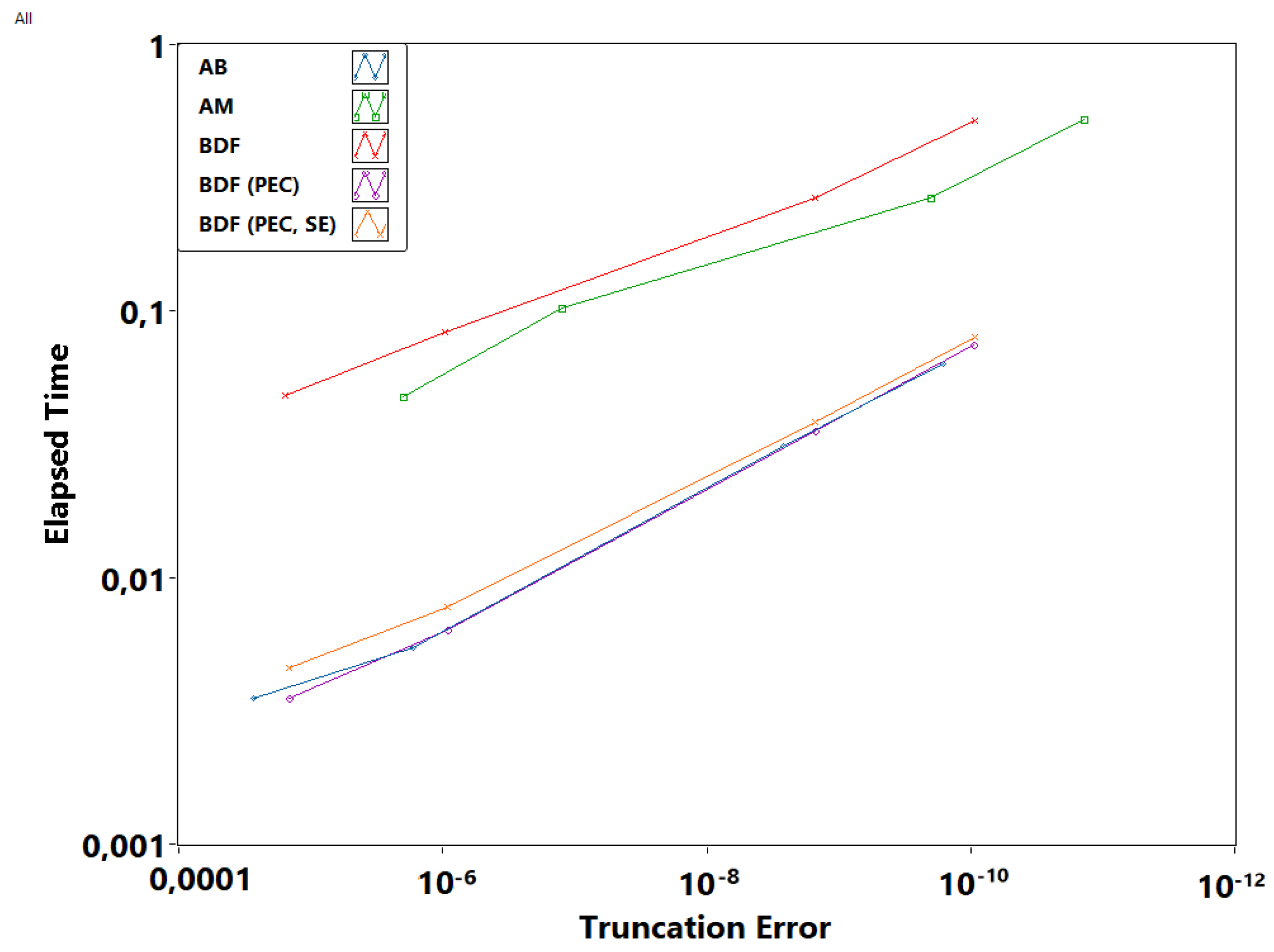
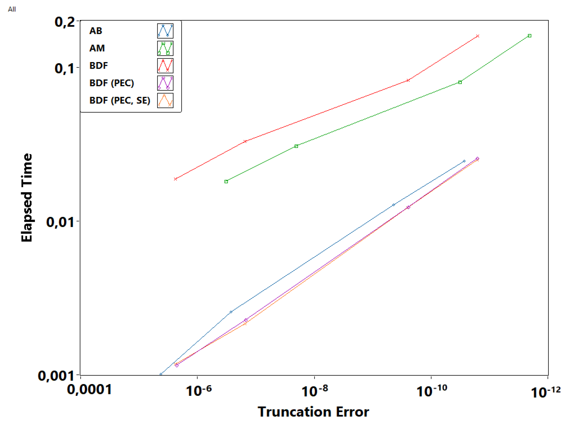
2.4. Test Problems for Estimating Method Performance

We use well-known test problems for estimating the method performance. The following methodology is used. The test ODE is solved with a given time step. In the final point of the simulation, an error is estimated through a comparison with a higher-order method, and the corresponding CPU time is measured. Experiments in several points give the line describing the method performance allowing the comparison with the other methods. More efficient methods are distinguished by a simple criterion: the lower the line lies, the more efficient the method is. We use DOPRI8 as the high-order method for obtaining a reference solution. All investigated algorithms are of the order 4. In order to avoid the influence of the operating system processes during CPU time measurements, this time was averaged over 10 independent simulations. The following methods are compared: Adams–Bashforth (AB), Adams–Moulton (AM), BDF, semi-implicit predictor–corrector BDF (BDF (PEC)), semi-explicit predictor–corrector BDF (BDF (PEC, SE)).
The first investigated test problem is the renown Rössler chaotic Equation [19]:
x ˙ =   y     z , y ˙ =   x   +   a y , z ˙ =   b   +   z ( x c ) ,
In our experiments, we used the classical parameters of the Rössler system a = 0.2 , b = 0.2, c = 5.7 . Initial conditions are ( 0.1 , 0 , 0.1 ) . The period of simulation is 50 s. The stepsizes under investigation are { 5 × 10 4 , 10 3 , 5 × 10 3 , 0.01 } s.
The second investigated test problem is the Nosé–Hoover chaotic Equation [20]:
x ˙ =   y , y ˙ =   x     a y z , z ˙ =   b ( y 2 1 ) ,
The parameters used are a   =   1 ,   b   =   1   and   c   =   5.7 . The initial conditions are ( 0.1 , 0 , 0.1 ) . The period of simulation lasted 15 s. The stepsizes under investigation are { 5 × 10 4 , 10 3 , 5 × 10 3 , 0.01 } s.
The third test problem is the van der Pol oscillator Equation [21]:
x ˙ =   y , y ˙ =   μ ( 1 x 2 ) y     x ,
The parameter used is μ   =   55 . Initial conditions are ( 1 , 0 ) . The period of simulation lasted 15 s. Stepsizes under investigation are { 10 5 , 5 × 10 5 , 10 4 , 5 × 10 4 } s.

3. Results

In this section, we provide the stability regions of the semi-explicit, semi-implicit ABM and BDF (PEC) predictor–corrector methods for k   =   [ 0 , 0.5 , 1 ] . In each figure, the stability regions of the methods of order 1–6 are depicted. Figure 1 shows the Adams–Bashforth–BDF predictor–corrector semi-explicit method stability regions, and Figure 2 shows the Adams–Bashforth–BDF predictor–corrector semi-implicit method stability regions.
In Figure 3, one can see that the region of stability for the semi-explicit method is smaller for the order 1 than the order 2 near the real axis. The method is, therefore, less interesting to be used in the order 1. The region decreases as the order of accuracy increases and the higher-order regions are included in the smaller order ones (except for p   =   1 ).
For the semi-implicit method, it seems that order 1 covers the negative real axis or at least large negative numbers in absolute value for k   =   0.5 , 1 . Contrary to the previous method, the first order of the semi-implicit ABM method has a greater stability region than the following orders. However, it retains some common characteristics: from order 4, the stability region does not include the positive real part. Moreover, the stability region decreases when the order of the method increases, and the stability region of an order is included in the one of the previous order. These characteristics are common to all three methods, which is due the semi-explicit (Figure 3) and semi-implicit (Figure 4) methods modifying the ABM method (Figure 5).
Note that the stability region of the semi-implicit method is strictly included in the stability region of the implicit AM method (Figure 6) in the left part of the complex plane (i.e., for stable problems).
Similar conclusions can be drawn for k   =   0 and k   =   0.5 , as can be seen in Figure 3 for the semi-explicit method and Figure 4 for the semi-implicit method. Moreover, based on the stability regions for those three values of k, we can stress that k   =   0.5 is an intermediate case between k   =   0 and k   =   1 . Finally, comparing the two extreme cases shows that case k   =   0 is the worst case for the numerical stability of the two modifications of ABM, whereas k   =   1 is the best case. Obviously, the ABM method is not impacted by the value of k.
The stability regions of the BDF (PEC) semi-explicit method are given in Figure 1. Its size in the imaginary axis is sufficiently greater than the size of any other investigated method which makes it more feasible for moderately stiff problems. The BDF (PEC) semi-implicit method with the stability region shown in Figure 2 has an approximately similar size in the imaginary axis as its semi-explicit counterpart has a much greater size in real axes. Thus, among all considered semi-explicit and semi-implicit methods, a family of semi-implicit BDF (PEC) methods has the largest stability regions, and for high orders, they are even greater than the stability regions of Adams–Moulton methods.
Performance tests show that on the test problems described above, the semi-implicit predictor–corrector BDF (BDF (PEC)) and semi-explicit predictor–corrector BDF (BDF (PEC, SE))) show the best error-to-CPU time ratio in comparison with conventional multistep methods: Adams–Bashforth (AB), Adams–Moulton (AM), and backward differentiation formula (BDF). The first test on the Rössler test problem (Figure 7) shows that the BDF and AB methods are the best for the problem. This is due to the low stiffness of the problem and using constant stepsizes. The Nosé–Hoover test problem (Figure 8) is a type of conservative chaotic problem. While the AB method preserved its high performance, the proposed predictor–corrector BDF methods have the advantage over it and other methods. The van der Pol oscillator (Figure 9) with μ   =   15 is moderately stiff but it also allows BDF PEC methods with constant stepsizes to outperform all the other methods.

4. Discussion and Conclusions

In this paper, a stability analysis of the semi-implicit and semi-explicit predictor–corrector methods was performed. We clearly show that the semi-explicit and semi-implicit ABM and BDF (PEC) methods expand the stability regions over the conventional ABM method and thus have better numerical stability. As one can see in Figure 2 and Figure 3, for the test problem with a matrix in the Jordan normal form ( k   =   1 ), the stability regions of all considered methods are wider in the complex plane than those of the ABM method regardless of the order or method. For the intermediate case ( k   =   0.5 ), we observe a similar situation. For the worst case, i.e., k   =   0 when the matrix is in the Frobenius form, then this is not true. For example, in Figure 3, the semi-explicit ABM method obtains a smaller stability region than the ABM method. In a similar case, k   =   0 the semi-implicit ABM method obtains stability regions relatively comparable to that of ABM.
It is well-known that the original BDF is A ( α ) -stable, while this stability is bought by the high costs of fully implicit computation involving Newton’s method. In the case of the semi-explicit method, no truly implicit computation is needed, while the stability regions are almost as wide in imaginary directions as the stability regions of the AM methods for p     3 . This allows using the BDF (PEC) semi-explicit method in many problems where the conventional AM method is used, with less computational efforts. As for the semi-implicit BDF (PEC) method, it has a very large negative real part of stability regions in the case of values of k close to 1, which make it especially attractive for the problems with symmetric Jacobian matrices. It should be noted that using the DF (PEC) methods requires twice the amount of memory compared to using ABM. However, these algorithms can be further optimized using the approach given in [17].
For the problems at the boundary of stability, when the eigenvalues are purely imaginary, the ABM methods are interesting up to the order of 5 and BDF (PEC) is interesting up to the order of 6 because they have a part of the imaginary axis in their region of stability. A simple example of the problem with purely imaginary eigenvalues is the pendulum without friction. However, a key difference in the stability of the semi-explicit and semi-implicit methods is that BDF is not stable for orders greater than 6, while Adams–Bashforth and Adams–Moulton methods can be used with much higher orders with sufficiently small stepsizes.
The overall results show that, in the worst case, we lose less stability than we can gain in the intermediate and best cases, which is evidence of the potential superiority of the semi-explicit and semi-implicit methods over conventional AM and ABM algorithms.
In terms of computational efficiency, ref. [17] showed that semi-explicit and semi-implicit ABM methods are efficient methods compared to other linear multistep methods (such as ABM and BDF). Furthermore, it was shown in [17] that semi-explicit and semi-implicit ABM methods are sufficiently flexible to optimize the computations according to the problem features. The comparison of the error-to-CPU time ratio of the semi-explicit and semi-implicit predictor–corrector BDF methods was performed in the current paper with the other multistep methods. It was shown that these methods have a superior error-to-CPU time ratio in the experiments with constant stepsize, and this superiority could be even more valuable for variable stepsizes. Further investigation is needed to compare variable stepsize implementations.
The motivation of semi-implicit computation is that each equation can be solved separately, so implicit algebraic equations must be solved for one variable, and the computation of the full Hessian matrix in the Newton method is not required. Moreover, some one-dimensional variants of root-finding algorithms can also be used such as Brent’s method or Steffensen’s method. Note that, in some cases, the computational cost can be further optimized. For instance, ref. [15] described a problem for which an equation of the corrector can be solved independently of the previous computations of the corrector. Furthermore, for the semi-implicit method, the predictor of the first variable does not need to be computed; therefore, one can choose the order of the equations in the system (1) to decrease the computational cost excluding the computationally “heavy” right-hand side function evaluation.
Finally, applying the semi-explicit and semi-implicit methods to other problems such as fractional-order differential equations could be one of the possible directions for further investigations. Numerical approaches to solving this type of problem studied in [7,22,23] applied the Adams–Bashforth explicit method. Thus, using the semi-explicit and semi-implicit modified ABM methods may be a new application in the continuation of these articles.

Author Contributions

Conceptualization, A.T. and D.B.; methodology, D.B.; software, A.T., L.B. and O.C.; validation, A.T., D.B., L.B., O.C. and V.L.; formal analysis, D.B.; investigation, A.T.; resources, A.T.; data curation, A.T.; writing—original draft preparation, L.B., O.C. and D.B.; writing—review and editing, A.T. and V.L.; visualization, L.B. and O.C.; supervision, V.L.; project administration, D.B. All authors have read and agreed to the published version of the manuscript.

Funding

This study was supported by the grant of the Russian Science Foundation (RSF), project 22-19-00573.

Institutional Review Board Statement

Not applicable.

Informed Consent Statement

Not applicable.

Data Availability Statement

Not applicable.

Conflicts of Interest

The authors declare no conflict of interest.

Abbreviations

The following abbreviations are used in this manuscript:
ODEOrdinary differential equations
BDFBackward differentiation formula
SIRKSingly implicit Runge–Kutta
DIRKDiagonally implicit Runge–Kutta
ABMAdams–Bashforth–Moulton
AMAdams–Moulton

References

  1. Awrejcewicz, J. Ordinary Differential Equations and Mechanical Systems; Springer: Cham, Switzerland, 2014. [Google Scholar]
  2. Cardelli, L.; Tribastone, M.; Tschaikowski, M. From electric circuits to chemical networks. Nat. Comput. 2020, 19, 237–248. [Google Scholar] [CrossRef]
  3. Cardelli, L. From Processes to ODEs by Chemistry. In Proceedings of the Fifth IFIP International Conference On Theoretical Computer Science—TCS 2008, IFIP International Federation for Information Processing, Milano, Italy, 7–10 September 2008; Ausiello, G., Karhumäki, J., Mauri, G., Ong, L., Eds.; Springer: Boston, MA, USA, 2008. [Google Scholar]
  4. Polynikis, A.; Hogan, S.J.; Di Bernardo, M. Comparing different ODE modelling approaches for gene regulatory networks. J. Theor. Biol. 2009, 261, 511. [Google Scholar] [CrossRef] [PubMed]
  5. Keeling, M.; Rohani, P. Modeling Infectious Diseases in Humans and Animals; Princeton University Press: Princeton, NJ, USA, 2008. [Google Scholar]
  6. Hairer, E.; Nørsett, S.P.; Wanner, G. Solving Ordinary Differential Equations I: Nonstiff Problems, 2nd ed.; Springer: Berlin, Germany, 1993; pp. 427–429. [Google Scholar]
  7. Jafari, H.; Ganji, R.M.; Nkomo, N.S.; Lv, Y.P. A numerical study of fractional order population dynamics model. Results Phys. 2021, 27, 104456. [Google Scholar] [CrossRef]
  8. Faleichik, B.V. Minimal residual multistep methods for large stiff non-autonomous linear problems. J. Comput. Appl. Math. 2019, 389, 112498. [Google Scholar] [CrossRef]
  9. Karimov, A.I.; Butusov, D.N.; Tutueva, A.V. Adaptive explicit-implicit switching solver for stiff ODEs. In Proceedings of the IEEE Conference of Russian Young Researchers in Electrical and Electronic Engineering (EIConRus), St. Petersburg and Moscow, Russia, 1–3 February 2017; pp. 440–444. [Google Scholar]
  10. Lopez, S. A predictor-corrector time integration algorithm for dynamic analysis of nonlinear systems. Nonlinear Dynynamics 2020, 101, 1365–1381. [Google Scholar] [CrossRef]
  11. Hairer, E.; Wanner, G. Solving Ordinary Differential Equations II: Stiff and Differential-Algebraic Problems, 2nd ed.; Springer: Berlin, Germany, 1993; pp. 91–100, 128–130. [Google Scholar]
  12. Rauber, T.; Rünger, G. Parallel Implementations of Iterated Runge-Kutta Methods. Int. J. Supercomput. Appl. High Perform. Comput. 1996, 10, 62–90. [Google Scholar] [CrossRef]
  13. Liu, C.; Wu, H.; Feng, L.; Yang, A. Parallel Fourth-Order Runge-Kutta Method to Solve Differential Equations. In Proceedings of the ICICA 2011: Information Computing and Applications, Qinhuangdao, China, 28–31 October 2011; Lecture Notes in Computer Science. Springer: Berlin, Germany, 2011; Volume 7030. [Google Scholar]
  14. Press, W.H.; Teukolsky, S.A.; Vetterling, W.T.; Flannery, B.P. The Art of Scientific Computing, 3rd ed.; Cambridge University Press: Cambridge, UK, 2007. [Google Scholar]
  15. Tutueva, A.; Karimov, T.; Butusov, D. Semi-Implicit and Semi-Explicit Adams-Bashforth-Moulton Methods. Mathematics 2020, 8, 780. [Google Scholar] [CrossRef]
  16. Cellier, F.E.; Kofman, E. Continuous System Simulation; Springer: Berlin/Heidelberg, Germany, 2006. [Google Scholar]
  17. Tutueva, A.; Butusov, D. Stability Analysis and Optimization of Semi-Explicit Predictor–Corrector Methods. Mathematics 2021, 9, 2463. [Google Scholar] [CrossRef]
  18. Butusov, D.; Karimov, A.; Andreev, V.; Ostrovskii, V. Semi-Explicit Composition Methods in Memcapacitor Circuit Simulation. Int. J. Embed. Real-Time Commun. Syst. 2019, 10, 37–52. [Google Scholar] [CrossRef]
  19. Rössler, O.E. An equation for continuous chaos. Phys. Lett. A 1976, 57, 397–398. [Google Scholar] [CrossRef]
  20. Posch, H.A.; Hoover, W.; Vesely, F.J. Canonical dynamics of the Nosé oscillator: Stability, order, and chaos. Phys. Rev. A 1986, 33, 4253–5265. [Google Scholar] [CrossRef]
  21. van der Pol, B. The nonlinear theory of electric oscillations. Proc. Inst. Radio Eng. 1934, 22, 1051–1086. [Google Scholar] [CrossRef]
  22. Zhang, A.; Ganji, R.M.; Jafari, H.; Ncube, M.N.; Agamalieva, L. Numerical Solution of Distributed-Order Integro-Differential Equations. Fractals 2021. [Google Scholar] [CrossRef]
  23. Kadkhoda, N.; Jafari, H.; Ganji, R.M. A numerical solution of variable order diffusion and wave equations. Int. J. Nonlinear Anal. Appl. 2021, 12, 27–36. [Google Scholar]
Figure 1. Stability regions of Adams–Bashforth–BDF semi-explicit methods with k   =   [ 0 , 0.5 , 1 ] (from left to right).
Mathematics 10 02015 g001
Figure 2. Stability regions of Adams–Bashforth–BDF semi-implicit methods with k   =   [ 0 , 0.5 , 1 ] (from left to right).
Mathematics 10 02015 g002
Figure 3. Stability regions of the semi-explicit ABM method with k   =   [ 0 , 0.5 , 1 ] (from left to right).
Mathematics 10 02015 g003
Figure 4. Stability regions of the semi-implicit ABM method for k   =   [ 0 , 0.5 , 1 ] (from left to right).
Mathematics 10 02015 g004
Figure 5. Stability regions of the Adams–Bashforth–Moulton predictor–corrector method.
Mathematics 10 02015 g005
Figure 6. Stability regions of the Adams–Moulton method.
Mathematics 10 02015 g006
Figure 7. Comparison of the error versus elapsed time for the family of investigated methods on the test Rössler problem.
Mathematics 10 02015 g007
Figure 8. Comparison of the error versus elapsed time for the family of investigated methods on the Nosé–Hoover problem.
Mathematics 10 02015 g008
Figure 9. Comparison of the error versus elapsed time for the family of investigated methods on the van der Pol oscillator problem.
Mathematics 10 02015 g009
Table 1. Coefficients of the Adams–Bashforth–backward differentiation method.
B 1 B 2 B 3 B 4 B 5 B 6
100000
3/2−1/20000
23/12−16/125/12000
55/24−59/2437/24−9/2400
1901/720−2774/7202616/720−1274/720251/7200
4277/1440−7923/14409982/1440−7298/14402877/1440−475/1440
α 1 α 2 α 3 α 4 α 5 α 6
−100000
−4/31/30000
−18/119/11−2/11000
−48/2536/25−16/253/2500
−300/137300/137−200/13775/137−12/1370
−360/147450/147−400/147225/147−72/14710/147
β 1 β 2 β 3 β 4 β 5 β 6
12/36/1112/2560/13760/147
Publisher’s Note: MDPI stays neutral with regard to jurisdictional claims in published maps and institutional affiliations.

