Author Contributions
Conceptualization, J.V.-E., J.C.-R. and I.U.-M.; Formal analysis, J.V.-E., J.C.-R. and I.U.-M.; Investigation, J.V.-E., J.C.-R., V.G.-P. and I.U.-M.; Methodology, J.V.-E., J.C.-R. and I.U.-M.; Software, J.V.-E., J.C.-R., V.G.-P. and I.U.-M.; Supervision, J.V.-E., J.C.-R. and I.U.-M.; Validation, J.V.-E. and I.U.-M.; Writing—original draft, J.V.-E., J.C.-R. and I.U.-M.; Writing—review & editing, J.V.-E., J.C.-R., V.G.-P. and I.U.-M. All authors have read and agreed to the published version of the manuscript.
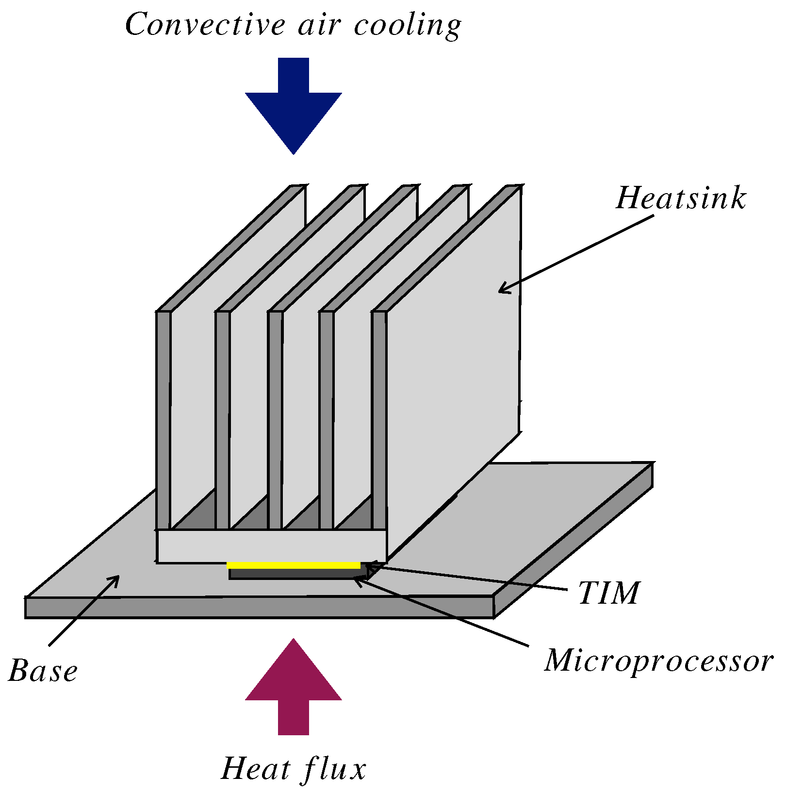
Figure 1.
Typical low heat generation microelectronic packaging architecture.
Figure 1.
Typical low heat generation microelectronic packaging architecture.
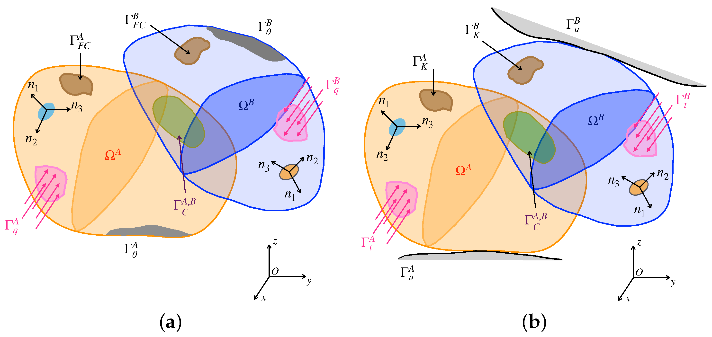
Figure 2.
(a) Schema of the thermal problem. (b) Schema of the elastic problem.
Figure 2.
(a) Schema of the thermal problem. (b) Schema of the elastic problem.
Figure 3.
(a) Equivalent thermal contact resistance model for no TIM consideration. (b) Equivalent thermal contact resistance model for TIM consideration.
Figure 3.
(a) Equivalent thermal contact resistance model for no TIM consideration. (b) Equivalent thermal contact resistance model for TIM consideration.
Figure 4.
General thermal contact illustration and the schematic temperature distribution along the two bodies’ contact surfaces.
Figure 4.
General thermal contact illustration and the schematic temperature distribution along the two bodies’ contact surfaces.
Figure 5.
Local coordinate system of each pair of elements in contact.
Figure 5.
Local coordinate system of each pair of elements in contact.
Figure 6.
(a) Proposed geometry and initial boundary conditions. (b) New elastic boundary conditions.
Figure 6.
(a) Proposed geometry and initial boundary conditions. (b) New elastic boundary conditions.
Figure 7.
Discretization influence on the normal contact traction and temperature values at the nodes located at the diagonal of the contact zone for: elements, elements and elements.
Figure 7.
Discretization influence on the normal contact traction and temperature values at the nodes located at the diagonal of the contact zone for: elements, elements and elements.
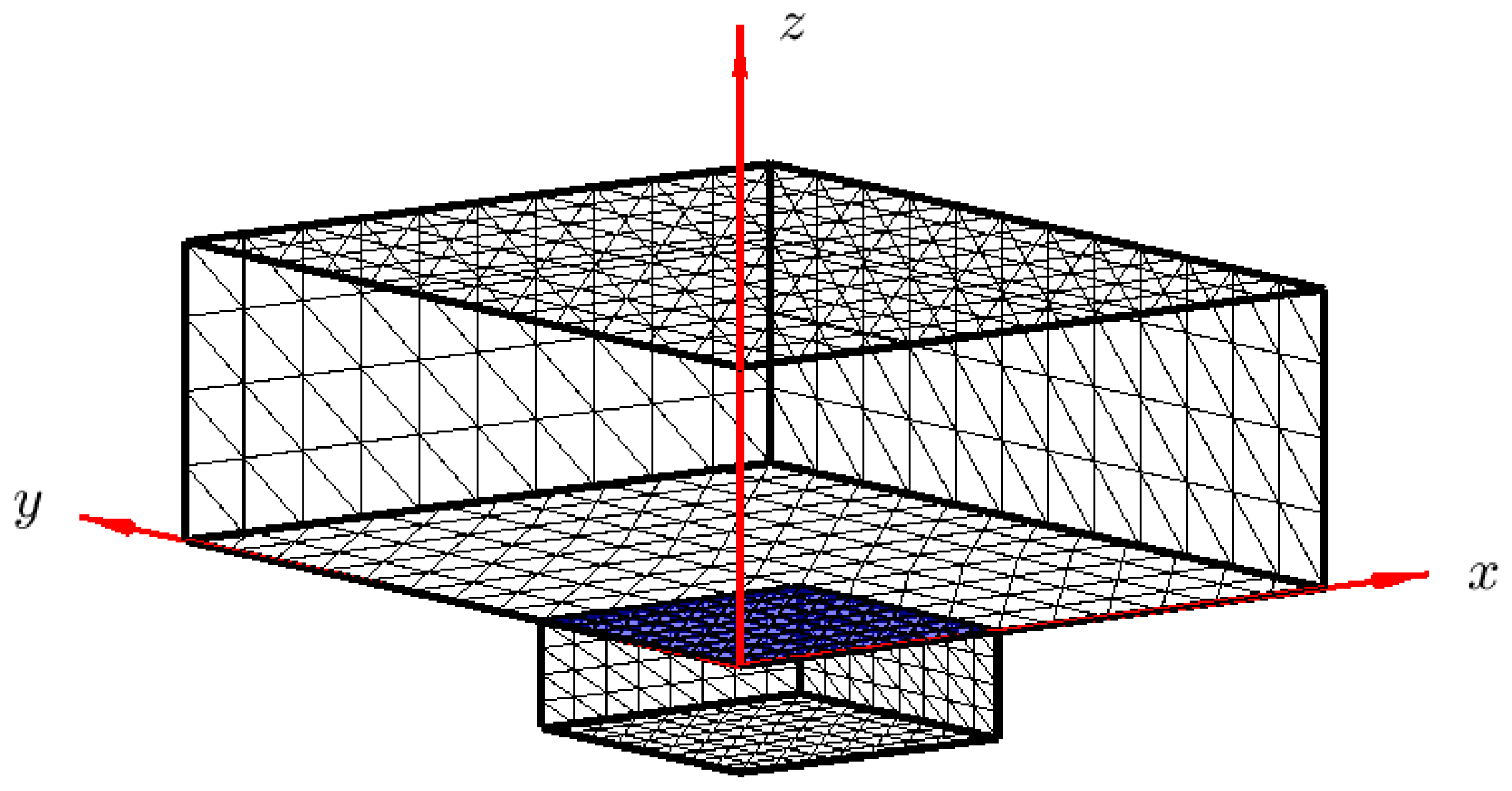
Figure 8.
Microelectronic packaging boundary BEM mesh chosen.
Figure 8.
Microelectronic packaging boundary BEM mesh chosen.
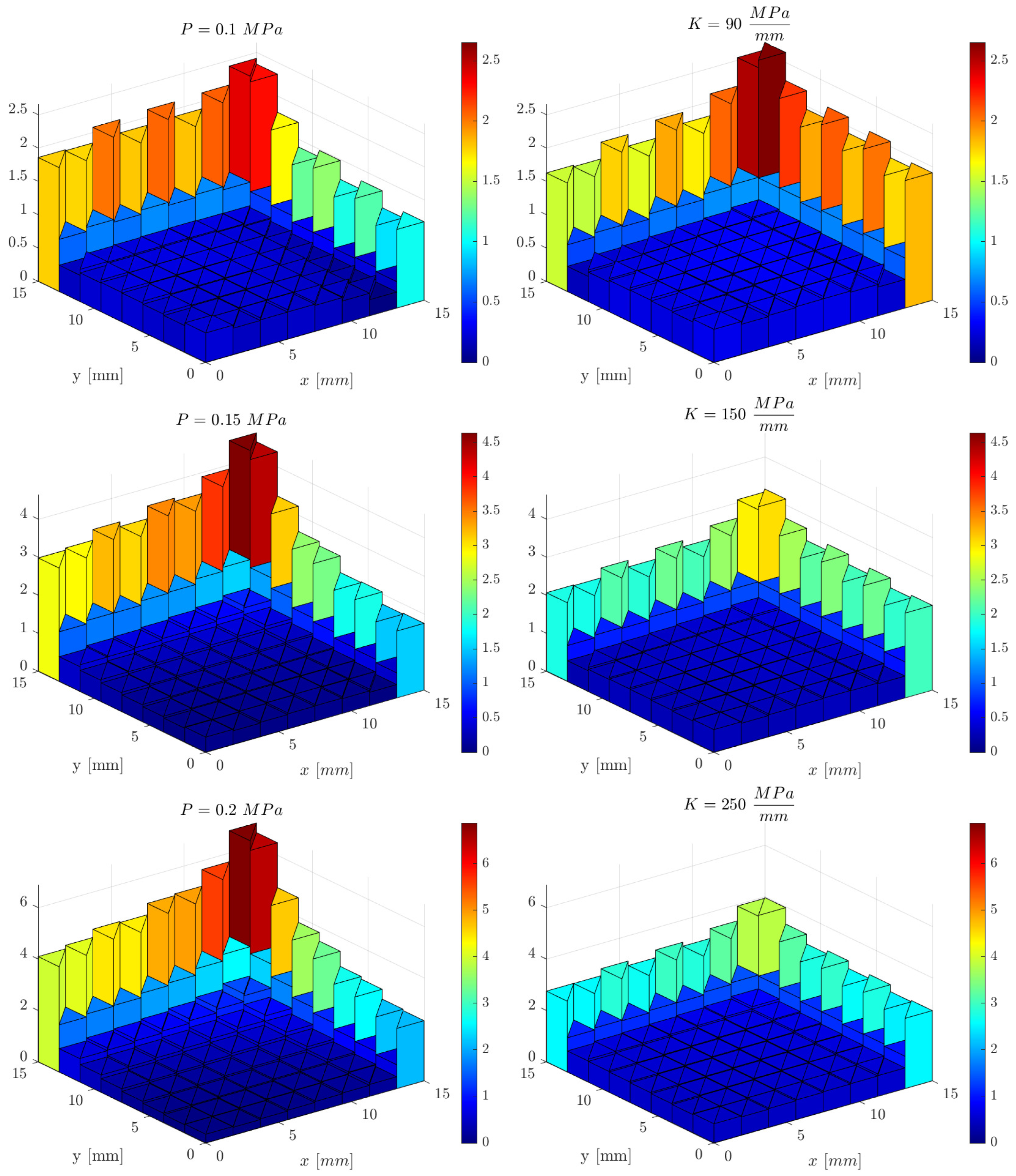
Figure 9.
Normal contact traction distribution comparsion at the nodes located at the diagonal of the contact zone for the uniform clamping pressure and Winkler elastic supports.
Figure 9.
Normal contact traction distribution comparsion at the nodes located at the diagonal of the contact zone for the uniform clamping pressure and Winkler elastic supports.
Figure 10.
Thermal contact resistance comparison at the nodes located at diagonal of the contact zone for the uniform clamping pressure and Winkler elastic supports.
Figure 10.
Thermal contact resistance comparison at the nodes located at diagonal of the contact zone for the uniform clamping pressure and Winkler elastic supports.
Figure 11.
Temperature distribution comparison at the elements located at the diagonal of the base of the microprocessor for the uniform clamping pressure and Winkler elastic supports.
Figure 11.
Temperature distribution comparison at the elements located at the diagonal of the base of the microprocessor for the uniform clamping pressure and Winkler elastic supports.
Figure 12.
Model analyzed in this example where the influence of different TIMs is analyzed.
Figure 12.
Model analyzed in this example where the influence of different TIMs is analyzed.
Figure 13.
(a) Median normal contact traction value comparison at the potential contact zone. (b) Normal contact traction distribution comparison at the nodes located at the diagonal of the contact zone.
Figure 13.
(a) Median normal contact traction value comparison at the potential contact zone. (b) Normal contact traction distribution comparison at the nodes located at the diagonal of the contact zone.
Figure 14.
Thermal contact resistance distribution comparison at the nodes located at the diagonal of the contact zone.
Figure 14.
Thermal contact resistance distribution comparison at the nodes located at the diagonal of the contact zone.
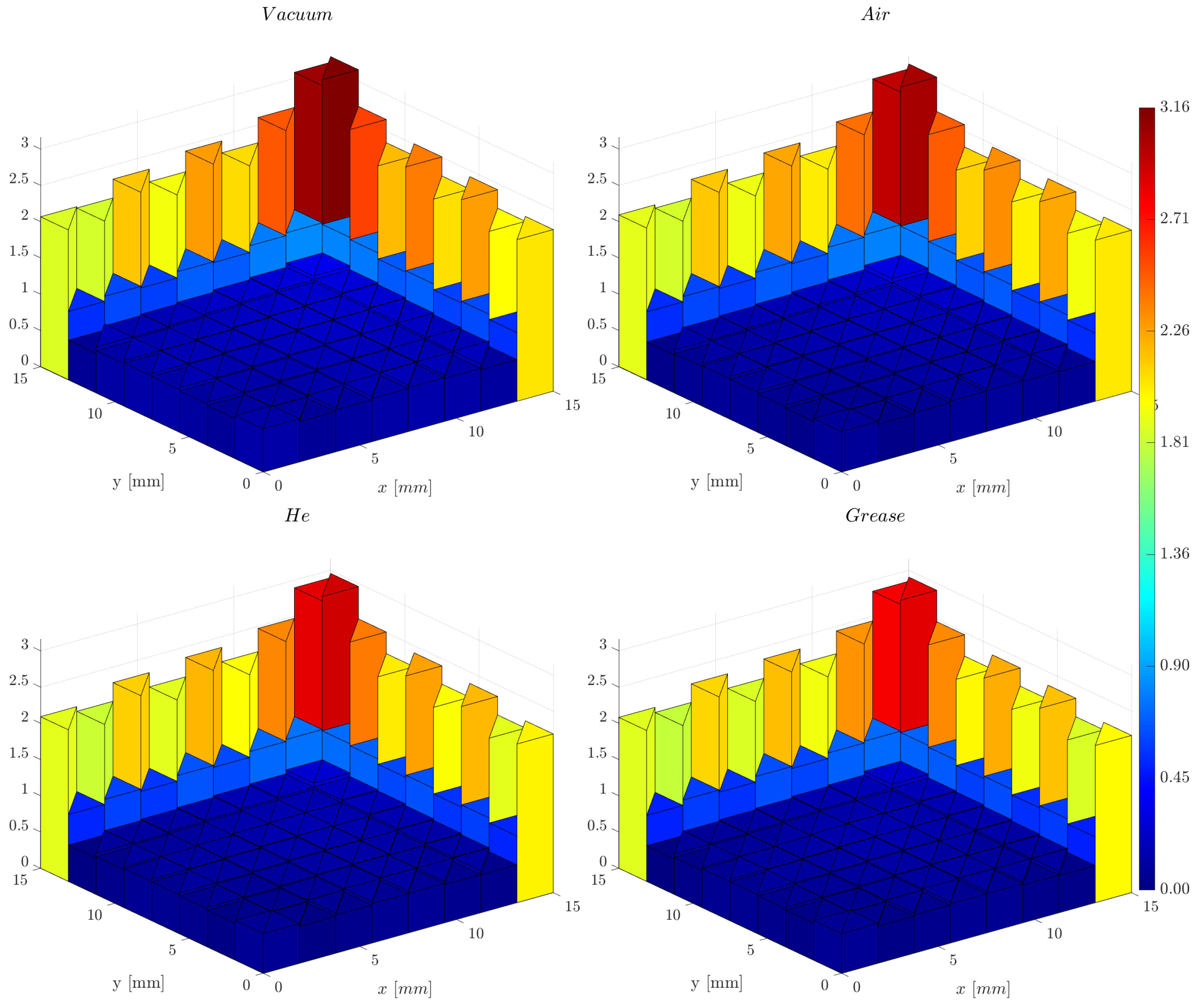
Figure 15.
Microcontacts thermal contact conductance () and TIM thermal conductance () % comparison for all TIMs studied at the potential contact zone.
Figure 15.
Microcontacts thermal contact conductance () and TIM thermal conductance () % comparison for all TIMs studied at the potential contact zone.
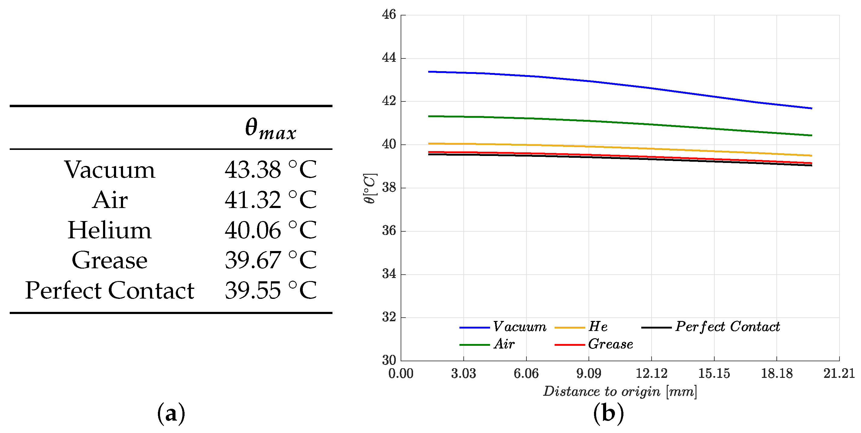
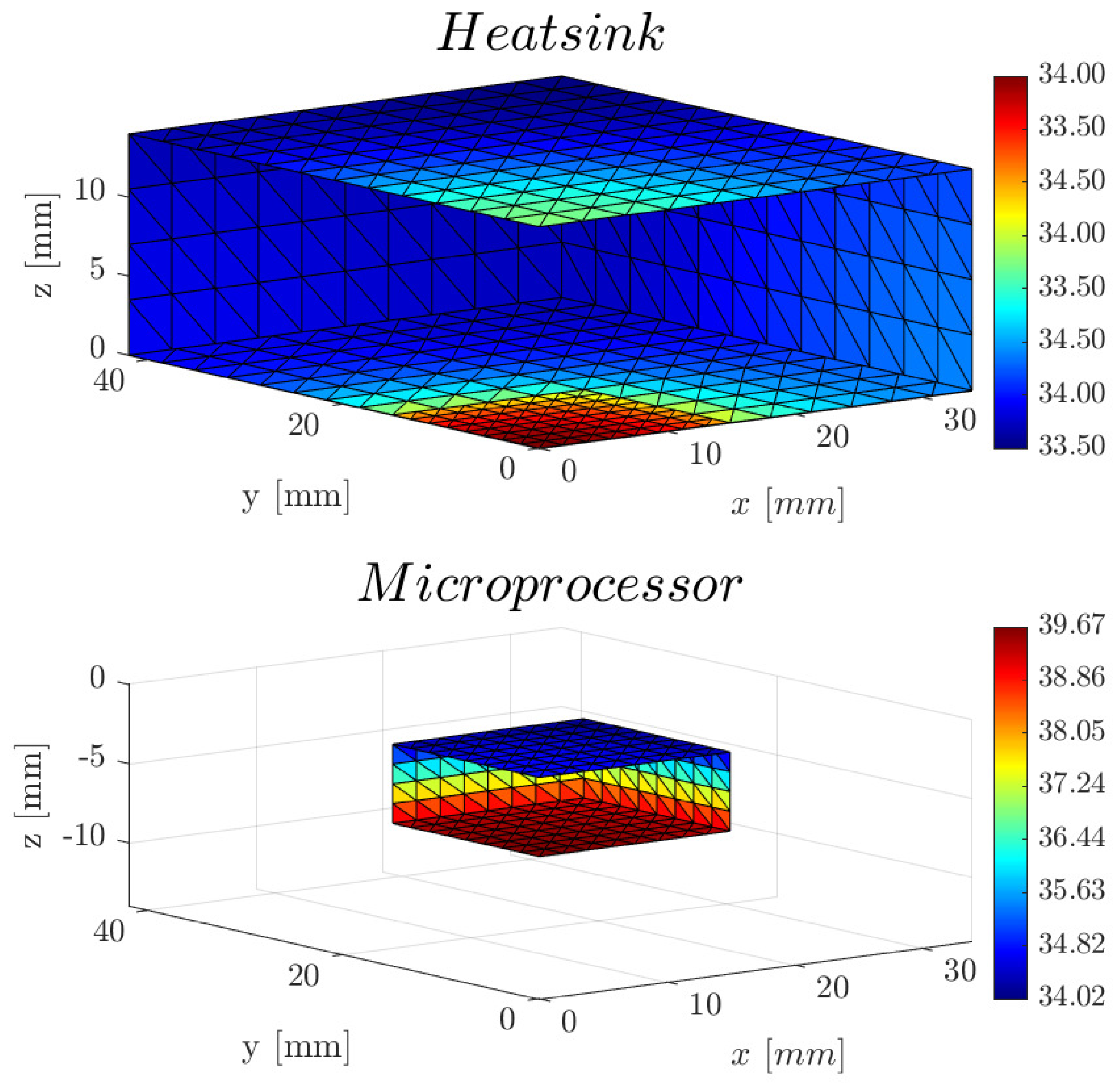
Figure 16.
(a) Maximum temperature values comparison on the base of the microprocessor for each TIM analyzed. (b) Temperature distribution comparison at the nodes located at the diagonal of the base of the microprocessor.
Figure 16.
(a) Maximum temperature values comparison on the base of the microprocessor for each TIM analyzed. (b) Temperature distribution comparison at the nodes located at the diagonal of the base of the microprocessor.
Figure 17.
Model analyzed in this example where a thermal grease is introduced at the interface and the effect of different Winkler elastic support stiffness K and is analyzed.
Figure 17.
Model analyzed in this example where a thermal grease is introduced at the interface and the effect of different Winkler elastic support stiffness K and is analyzed.
Figure 18.
Normal traction distribution at the nodes located at the diagonal of the contact zone of all the stiffness of the retaining mechanism analyzed for: W, W, W and W.
Figure 18.
Normal traction distribution at the nodes located at the diagonal of the contact zone of all the stiffness of the retaining mechanism analyzed for: W, W, W and W.
Figure 19.
Temperature distribution at the nodes located at the diagonal of the base of the microprocessor for: W, W, W and W.
Figure 19.
Temperature distribution at the nodes located at the diagonal of the base of the microprocessor for: W, W, W and W.
Figure 20.
Maximum temperature at the base of the microprocessor for: W, W, W and W.
Figure 20.
Maximum temperature at the base of the microprocessor for: W, W, W and W.
Figure 21.
Maximum temperature at the base of the microprocessor for different values of .
Figure 21.
Maximum temperature at the base of the microprocessor for different values of .
Figure 22.
C correlation as a function of .
Figure 22.
C correlation as a function of .
Figure 23.
Possible microelectronic packaging architecture for high-generation conditions.
Figure 23.
Possible microelectronic packaging architecture for high-generation conditions.
Table 1.
Case study summary.
Table 1.
Case study summary.
| Case | Initial Situation | Enhancements |
|---|
| 1 | | |
| 2 | | |
| 3 | | |
Table 2.
Equivalent Winkler elastic support stiffness.
Table 2.
Equivalent Winkler elastic support stiffness.
| Clamping Pressure [MPa] | K [MPa/mm] |
|---|
| 0.1 | 90 |
| 0.15 | 150 |
| 0.2 | 250 |
Table 3.
Material properties of the microelectronic packaging.
Table 3.
Material properties of the microelectronic packaging.
| | Processor | Heatsink |
|---|
| E [MPa] | | |
| | |
| [°C−1] | | |
| k [] | | |
| H [MPa] | 1207 | 1094 |
| [mm] | | |
| m | | |
Table 4.
Median normal contact traction comparison for different uniform clamping pressures P and Winkler elastic support stiffness K.
Table 4.
Median normal contact traction comparison for different uniform clamping pressures P and Winkler elastic support stiffness K.
| P [MPa] | [MPa] | K [MPa/mm] | [MPa] |
|---|
| | 90 | |
| | 150 | |
| | 250 | |
Table 5.
Median thermal contact resistance comparison for the uniform clamping pressure P and Winkler elastic supports stiffness K.
Table 5.
Median thermal contact resistance comparison for the uniform clamping pressure P and Winkler elastic supports stiffness K.
| P [MPa] | [°Cmm2/W] | K [MPa/mm] | [°Cmm2/W] |
|---|
| | 90 | |
| | 150 | |
| | 250 | |
Table 6.
Maximum temperature at the base of the microprocessor comparison for the uniform clamping pressure P and Winkler elastic supports stiffness K.
Table 6.
Maximum temperature at the base of the microprocessor comparison for the uniform clamping pressure P and Winkler elastic supports stiffness K.
| P [MPa] | [°C] | K [MPa/mm] | [°C] |
|---|
| | 90 | |
| | 150 | |
| | 250 | |
Table 7.
Thermal interface material properties used to calculate the thermal contact resistance ().
Table 7.
Thermal interface material properties used to calculate the thermal contact resistance ().
| TIM | k [W/mm°C] | [mm] |
|---|
| Air | | |
| Helio | | |
| Grease | | |
Table 8.
Median microcontacts thermal contact conductance (
[W/°Cmm
2]) and TIM thermal conductance (
[W/°Cmm
2]) comparison for all TIMs studied calculated according to Equations (
8) and (
10).
Table 8.
Median microcontacts thermal contact conductance (
[W/°Cmm
2]) and TIM thermal conductance (
[W/°Cmm
2]) comparison for all TIMs studied calculated according to Equations (
8) and (
10).
| | | | | |
|---|
| Vacuum | | - | | |
| Air | | | | |
| Helium | | | | |
| Grease | | | | |
Table 9.
Microelectronic packaging thermal efficiency for each TIM analyzed.
Table 9.
Microelectronic packaging thermal efficiency for each TIM analyzed.
| | | |
|---|
| Vacuum | 43.38 °C | 0.00% |
| Air | 41.32 °C | 53.80% |
| Helium | 40.06 °C | 86.70% |
| Grease | 39.67 °C | 97.00% |
| Perfect Contact | 39.55 °C | 100.00% |
Table 10.
Heat q [W] generated at the base of the microprocessor and its respective maximum Winkler elastic support stiffness.
Table 10.
Heat q [W] generated at the base of the microprocessor and its respective maximum Winkler elastic support stiffness.
| (°C/mm) | q (W) | K (MPa/mm) |
|---|
| 1.00 | 18.81 | 150 |
| 1.50 | 28.22 | 75 |
| 2.00 | 37.62 | 10 |
| 2.50 | 47.03 | − |

 ,
, 


