
Modified Bernstein–Durrmeyer Type Operators


1
Department of Mathematics, Central University of Haryana, Mahendragarh 123029, Haryana, India
2
Department of Mathematics and Computer Science, Technical University of Cluj-Napoca, North University Center at Baia Mare, Victoriei 76, 430122 Baia Mare, Romania
*
Author to whom correspondence should be addressed.
Mathematics 2022, 10(11), 1876; https://doi.org/10.3390/math10111876
Submission received: 8 April 2022
/
Revised: 26 May 2022
/
Accepted: 27 May 2022
/
Published: 30 May 2022
Abstract
:We constructed a summation–integral type operator based on the latest research in the linear positive operators area. We establish some approximation properties for this new operator. We highlight the qualitative part of the presented operator; we studied uniform convergence, a Voronovskaja-type theorem, and a Grüss–Voronovskaja type result. Our subsequent study focuses on a direct approximation theorem using the Ditzian–Totik modulus of smoothness and the order of approximation for functions belonging to the Lipschitz-type space. For a complete image on the quantitative estimations, we included the convergence rate for differential functions, whose derivatives were of bounded variations. In the last section of the article, we present two graphs illustrating the operator convergence.
Keywords:
linear positive operators; uniform approximation; rate of convergence; modulus of continuityMSC:
41A25; 41A36; 26A151. Introduction
The polynomial approximation of continuous functions represents an important part of numerical analyses. It is based on a famous theorem, stated, proved, and published by Karl Weierstrass in 1885. The result expresses the possibility of uniform approximation for a continuous function f by polynomials, on a bounded and closed interval of the real axis, playing a fundamental role in the development of mathematical analyses. In 1912, Bernstein [1] constructed for the real-valued function the positive linear operators
as a remarkable tool for the proof of the Weierstrass approximation theorem. Bernstein polynomials (1) ushered in a new era of the approximation theory, inspiring thousands of interesting articles to date. Bernstein polynomials, together with Bézier curves, are used in computer-aided geometric designs and other areas of computer science. Powerful algorithms (i.e., due to their constructions and visualizations) are available in the literature. Some generalizations (approximation of integrable functions, approximation of measurable functions, degenerate Bernstein polynomials, classical Bernstein polynomials), as well as many other applications of the Bernstein polynomials (1), can be consulted in the excellent book [2]. An exceptional historical perspective is provided in [3] on the evolution of the Bernstein polynomials. The construction of the approximation processes (of linear positive operators) is in a continuous expansion, determined only by the versatility of the existing functions. Consequently, there are dozens of operators in the literature; new operators can be built, all with direct contributions to the uniform approximation of the function. An interesting new modification of the Bernstein operator was brought to light by Usta [4]; it is given by
where are the fundamental polynomials. In order to obtain an approximation process in the spaces of integrable functions on the interval , based on this new modification (2), for any non-negative fixed real parameter , we present the following Bernstein–Durrmeyer type operator
where and are the Beta functions. We should note that (3) is a summation–integral linear positive type operator and its construction is based on many attempts to verify the hypotheses of an approximation process. The aim of the present paper was to establish some approximation properties of the Bernstein–Durrmeyer type operator (3). We highlight the qualitative part of the presented operator, studying uniform convergence, a Voronovskaja-type theorem, and a Grüss–Voronovskaja-type result. Our subsequent study focuses on a direct approximation theorem using the Ditzian–Totik modulus of smoothness, on the order of approximation for functions belonging to the Lipschitz-type space. For a complete image about the quantitative estimations, we include the convergence rates for differential functions whose derivatives were of bounded variations. In the last section of the article, we present two graphs illustrating the operator convergence.
2. Auxiliary Results
Let be the set of positive integers and . In this section, we present some auxiliary results. Let be a nonempty interval of the real axis. We consider the space of all real-valued functions continuous on I, endowed with uniform norm . The mapping is called an operator. The operator L is linear if , for , . The operator L is positive if , for any , f being positive. The next quantities represent indispensable tools for the study of uniform approximation of the functions by linear positive operators:
- The images of the monomials (called also Korovkin test functions) by operator L, written , for .
- The central moments of order m, , for .
Below, we present two results concerning the computations of the monomials images, as well as the central moments by linear positive operator .
Lemma 1.
The Bernstein–Durrmeyer-type operators (3) hold:
Proof.
Achieving the presented results requires the ability to operate with different types of mathematical software (Maple or Mathematica). □
As for the central moments of the operators (3), for brevity, in the sequel, we will write , with , and .
Lemma 2.
For the Bernstein–Durrmeyer-type operators (3), they hold:
Proof.
We use the results in Lemma 1. Taking , for , and 4 into account, we obtain the desired equalities. The computations were performed with Maple software. □
Lemma 3.
For every , applying the limit as , we have
Proof.
The equalities follow directly from Lemma 2, by applying the limit as . □
Lemma 4.
For , we have
where is a positive constant depending on the non-negative fixed real parameter α.
Proof.
The second order central moment of the Bernstein–Durrmeyer type operator (3) (see the result in Lemma 2), can be written in the following form
with being a positive constant and . □
The following result provides the simplest and strongest criteria for establishing the convergence of a linear positive operator to the identity one. It was developed and demonstrated independently by three mathematicians: T. Popoviciu [5] in 1951, H. Bohman [6] in 1952, and P.P. Korovkin [7] in 1953.
Theorem 1.
Let be a sequence of linear positive operators, such that . If
such that , then for any and , uniformly on .
Remark 1.
This classical result is known in the literature as Bohman–Korovkin’s theorem, because Popoviciu’s contribution remained unknown for a long period of time.
The power of this qualitative result impressed many mathematicians and, hence, during the last seventy years, a considerable amount of research extended this theorem in different directions.
3. Main Results
In the following, we present a series of qualitative and quantitative results, which confirm that the linear positive operator (3) is an approximation process in the space of integrable functions on .
Theorem 2.
If , then uniformly on .
Proof.
Taking the results presented in Lemma 1 into account, we have
Next, applying Bohman–Korovkin–Popoviciu criterion (Theorem 1), it follows that
□
Theorem 3.
Let . If , then
Proof.
Using Taylor’s expansion of the function , we can write
being a bounded function, with . Applying the linear operator to the relation (5), we have
The Cauchy–Schwarz inequality for linear positive operators implies
Based on the uniform convergence proved in Theorem 2, we have = , once as . For every , we know from Lemma 3 that
Hence, it follows that
The results proved in Lemma 3:
leads us to
□
We present a Grüss–Voronovskaja-type result for the Bernstein–Durrmeyer-type operators.
Theorem 4.
Let . If , then
Proof.
The following relation holds
Next, using the uniform convergence from Theorem 2, the Voronovskaja-type theorem from Theorem 3, and the results presented in Lemma 3, we have
□
In order to present some quantitative estimates of the Bernstein–Durrmeyer type operators, we recall the definitions of the Ditzian–Totik first order modulus of smoothness and the appropriate K-functional, taken from [8]. Let and The first order modulus of smoothness is
and the appropriate K-functional is defined by
where and is the uniform norm on . It is known (from Theorem 3.1.2, [8]) that , which means that there exists a constant , such that
We establish the order of approximation with the aid of the Ditzian–Totik modulus of smoothness.
Theorem 5.
If and , then
with being defined in the Lemma 4 and C is a positive constant.
Proof.
Using the relation and the fact that Bernstein–Durrmeyer type operators (3) preserve constants (see Lemma 1), we may write
For any , we have
Therefore,
Combining (7)–(9) and applying the Cauchy–Schwarz inequality for linear positive operators, we have
Using the result presented in the Lemma 4, we have
It is clear that
where the relation (10) is used. Taking infimum on the right-hand side of the above relation over all , we may write
Taking into account, we have the desired estimate. □
Let us consider the Lipschitz-type space defined as:
Theorem 6.
If , then
Proof.
Using Hölder’s inequality with and , for we show that
□
Theorem 7.
If , then
Proof.
For any , we can write
Applying on both sides of the above relation, we have
Using the well-known inequality of modulus of continuity , , yields
Therefore,
Applying the Cauchy–Schwarz inequality for linear positive operators, we have
Choosing , the desired result follows. □
Let be the class of all absolutely continuous functions defined on , whose derivatives have bounded variation on . If , then
where , which means that g is a function with a bounded variation on . Moreover, the operators admit the integral representation
where the kernel is given by
Lemma 5.
For a fixed and sufficiently large n, it follows
(i)
(ii)
Proof.
Using the result from Lemma 4, we have
The proof’s argumentation is similar to ; hence, the details are omitted. □
Theorem 8.
Let ϕ. If and n is sufficiently large, then
where denotes the total variation of on and is defined by
Proof.
Since , using (13), for every we may write
If , then using (14) we have
with
Therefore,
By (13) and simple calculations we find
and
Using Lemma 4 and the relations (15), (16), we have
Let
To complete the proof, it is sufficient to determine the terms and Since for all applying the integration by parts and Lemma 5 with , we have
By the substitution of we have
Thus,
Using the integration by parts and Lemma 5 with we can write
By the substitution of we have
Combining (17)–(19), we obtain the desired relation. □
4. Numerical Examples
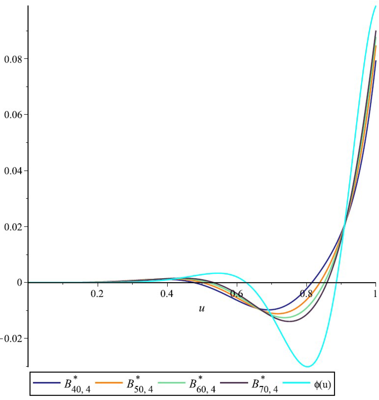
Example 1.
Figure 1 illustrates the convergence of the Bernstein–Durrmeyer type operators to the function , for various nodes, and a fixed parameter α.
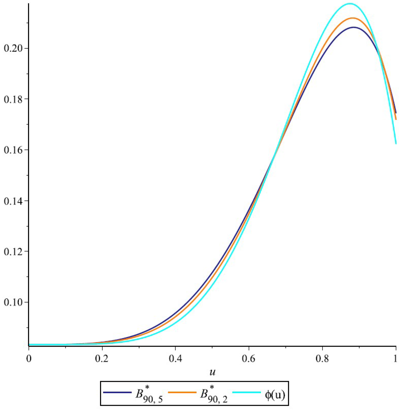
Example 2.
Figure 2 illustrates the convergence of the Bernstein–Durrmeyer type operators to the function , for various parameters, and a fixed number of nodes.
5. Conclusions
In this paper, we introduced a summation–integral linear positive-type operator. Any research related to the approximation of functions by linear positive operators involves highlighting two distinct parts. We proved the uniform convergence of the operators as well as a Voronovskaja-type theorem and Grüss–Voronovskaja-type results, which belong to the qualitative side. To obtain a complete picture of the quantitative estimates, we pointed out the orders of approximation of the new linear positive operators, using the Ditzian–Totik modulus of smoothness, as well as the convergence rate for differential functions whose derivatives were of bounded variations.
Author Contributions
Writing—original draft, A.K. and D.M. All authors have read and agreed to the published version of the manuscript.
Funding
The second author has been financially supported by Technical University of Cluj-Napoca.
Institutional Review Board Statement
Not applicable.
Informed Consent Statement
Not applicable.
Data Availability Statement
Not applicable.
Conflicts of Interest
The authors declare no conflict of interest.
References
- Bernstein, S.N. Demonstration du theoreme de Weierstrass fondee sur le calcul de probabilities. Comm. Soc. Math. Kharkov 1912, 13, 1–2. [Google Scholar]
- Lorentz, G.G. Bernstein Polynomials; University Toronto Press: Toronto, ON, Canada, 1953. [Google Scholar]
- Farouki, R. The Bernstein polynomial basis: A centennial retrospective. Comput. Aided Geom. Design 2012, 29, 379–419. [Google Scholar] [CrossRef]
- Usta, F. On New Modification of Bernstein Operators: Theory and Applications. Iran. J. Sci. Technol. Trans. Sci. 2020, 44, 1119–1124. [Google Scholar] [CrossRef]
- Popoviciu, T. Asupra demonstraţiei teoremei lui Weierstrass cu ajutorul polinoamelor de interpolare. In Lucrările Sesiunii Generale Şt. din 2–12 iunie 1950; Editura Academiei Republicii Populare Romane: Bucuresti, Romania, 1951; pp. 1–4, (translated into English by D. Kacsó, On the proof of Weierstrass theorem using intepolation polynomials. East J. Approx. 1998, 4, 107–110). [Google Scholar]
- Bohman, H. On approximation of continuous and of analytic function. Ark. Mat. 1952, 2, 43–56. [Google Scholar] [CrossRef]
- Korovkin, P.P. On the convergence of linear positive operators in the space of continuous functions. Dokl. Akad. Nauk. SSSR 1953, 90, 961–964. (In Russian) [Google Scholar]
- Ditzian, Z.; Totik, V. Moduli of Smoothness; Springer: New York, NY, USA, 1987. [Google Scholar]
Figure 1.
Approximation process.

Figure 2.
Approximation process.

Publisher’s Note: MDPI stays neutral with regard to jurisdictional claims in published maps and institutional affiliations. |
© 2022 by the authors. Licensee MDPI, Basel, Switzerland. This article is an open access article distributed under the terms and conditions of the Creative Commons Attribution (CC BY) license (https://creativecommons.org/licenses/by/4.0/).
Share and Cite
MDPI and ACS Style
Kajla, A.; Miclǎuş, D. Modified Bernstein–Durrmeyer Type Operators. Mathematics 2022, 10, 1876. https://doi.org/10.3390/math10111876
AMA Style
Kajla A, Miclǎuş D. Modified Bernstein–Durrmeyer Type Operators. Mathematics. 2022; 10(11):1876. https://doi.org/10.3390/math10111876
Chicago/Turabian StyleKajla, Arun, and Dan Miclǎuş. 2022. "Modified Bernstein–Durrmeyer Type Operators" Mathematics 10, no. 11: 1876. https://doi.org/10.3390/math10111876
Note that from the first issue of 2016, this journal uses article numbers instead of page numbers. See further details here.