Chaotic and Hyperchaotic Dynamics of a Clapp Oscillator

Abstract

This paper describes recent findings achieved during a numerical investigation of the circuit known as the Clapp oscillator. By considering the generalized bipolar transistor as an active element and after applying the search-for-chaos optimization approach, parameter regions that lead to either chaotic or hyperchaotic dynamics were discovered. For starters, the two-port that represents the transistor was firstly assumed to have a polynomial-forward trans-conductance; then the shape of trans-conductance changes into the piecewise-linear characteristics. Both cases cause vector field symmetry and allow the coexistence of several different attractors. Chaotic and hyperchaotic behavior were deeply analyzed by using standard numerical tools such as Lyapunov exponents, basins of attraction, bifurcation diagrams, and solution sensitivity. The structural stability of strange attractors observed numerically was finally proved via a real practical experiment: a flow-equivalent chaotic oscillator was constructed as the lumped electronic circuit, and desired attractors were captured and provided as oscilloscope screenshots.

1. Introduction

Roughly speaking, deterministic chaos can be considered as the unpredictable steady state of nonlinear dynamical systems with at least three degrees of freedom. By definition, this specific kind of solution possess two fundamental properties: it is sensitive to small changes of the initial conditions and bounded strange attractor with a non-integer geometric dimension. These two key features can be achieved simultaneously thanks to the suitable formation of the vector field and balanced distribution of dynamic energy over the state space. Moreover, from the perspective of chaotic and/or hyperchaotic circuits, a generated chaotic signal exhibits a continuous and broad-band frequency spectrum, caused by the presence of many unstable limit cycles. In further texts, chaotic phenomena will be related to a lumped electronic circuit with four accumulation elements. More precisely, analog building blocks dedicated for continuous-time signal generation will be addressed, both with respect to the generation of sinusoidal and chaotic waveforms.

The first lumped electronic circuit where the existence of a robust chaotic solution was confirmed theoretically, numerically, as well as experimentally was Chua’s oscillator [1]. It can be considered a parallel connection of the third-order passive ladder network and resistor having a piecewise linear (PWL) ampere–voltage (AV) characteristics. Without losing the chance to observe double-scroll, single-spiral, or other typical strange attractors, a PWL function can be substituted by a cubic polynomial function [2]. Both variants of Chua´s oscillator are still very popular for educational purposes because of their circuit simplicity, robustness of generated chaotic attractors, and easy-to-understand mechanisms behind chaos generation. Looking for the basic principle of chaos evolution, a harmonic oscillator can be considered as its core part. It is therefore understandable that many conventional topologies of the harmonic oscillators are investigated from the viewpoint of working regimes (system parameters, initial conditions), leading to the positive largest Lyapunov exponent (LE). Such a value usually indicates a solution that is sensitive to the small changes of the initial conditions, i.e., nearby trajectories diverge as time grows. One of the first examples of naturally non-chaotic oscillators turned into a generator of structurally stable chaotic attractors is described in paper [3]. There, the basic topology of the Colpitts oscillator is complemented by several additional elements including a voltage-controlled nonlinear resistor with two segment PWL AV curves. The author of a short paper [4] showed that this chaotic system could be mapped into Chua´s oscillator having an asymmetric PWL resistor. After the mutual exchange of capacitors and inductors in a typical Colpitts oscillator, we are experiencing Hartley´s structure. Inside this autonomous deterministic system, chaos was confirmed on an experimental basis in paper [5]. Another short work [6] analyzed a simple network that represents a bridge between Chua´s circuit and the Wien bridge oscillator. The contribution of the authors was that the active analog block that realizes the series connection of the negative inductor and resistor substitutes a classical inductor. A much more comprehensive study involving different topologies of Wien bridge-based chaotic oscillators is provided in paper [7]. A semi-systematic approach for the construction of chaos generators starting with the sinusoidal oscillator having a single current–feedback operational amplifier (AD844) is discussed in paper [8]. Despite the simplicity of discovered circuits, only simulation results are provided. The mentioned paper can be considered an extension of a much more comprehensive review [9]. Focusing on the phase shift sinusoidal oscillators, chaos can be successfully generated by a fully passive resistor–capacitor ladder terminated by a PWL resistor, as proved by author of paper [10]. Of course, this PWL resistor needs to be active, with at least one working area characterized by negative slope. From a practical realization point of view, the absence of inductors could be beneficial. Inductor-less circuitry realizations of third-order chaotic oscillators can be found in paper [11]. There, only two commercially available active elements are needed, and oscillators offer very simple relations between the parameters of mathematical models and values of circuit elements. Seen from different circuit-oriented perspectives, a single higher-order differential equation can be practically implemented as a closed loop of a passive low-pass filter and active two-port with polynomial transfer characteristics [12]. Besides “chaotic members” of class of sinusoidal oscillators, this kind of specific behavior has been reported in more complicated analog systems dedicated to continuous-time signal processing. One such example is phase-locked loop circuits, where chaos was firstly confirmed in paper [13]. After that, intensive research of phase-locked loops was performed, resulting into study [14]. Because of the existence of intrinsic nonlinearities, power electronics systems are ideal candidates where long chaotic transients as well as structurally stable chaotic oscillations can be observed. Many research papers were devoted to this problem. For example, papers [15] and [16] focused on the analysis of buck and boost DC–DC converters, respectively. A Cuk DC–DC converter was addressed in paper [17]. The rising of chaos phenomena in DC-DC converter, especially within a voltage-controlled buck converter, is explained in paper [18]. Difference equations, instead of differential equations, are derived and analyzed in the case of switching mode power converters. Consequently, conditions for the evolution of a discrete chaotic map are pronounced; see paper [19] for details. An analysis of a chaotic boost regulator that works in discontinuous modes is provided in paper [20]. Paper [21] shows that chaotic phenomena can be observed in a simple nonlinear switched-capacitor circuit. The analyzed system is described by a voltage–charge equation, i.e., it is discrete time dynamics. Interestingly, describing equations can be transformed into well-known logistic equations.

This paper extends the list of the well-known harmonic oscillators that are eventually capable of producing robust chaotic waveforms by one item, the Clapp oscillator. The next section describes a mathematical model of the original and chaotic Clapp oscillator, i.e., a generally autonomous, deterministic fourth-order dynamical system having three linear capacitors and one inductor. The third section covers an analysis of the simplified Clapp oscillator using standard numerical algorithms (LE, bifurcation diagrams, basins of attraction). The fourth part of this paper shows that chaotic movement is neither long transient nor a numerical artifact. Finally, concluding remarks and a few suggestions for future work are provided.

2. Mathematical Models

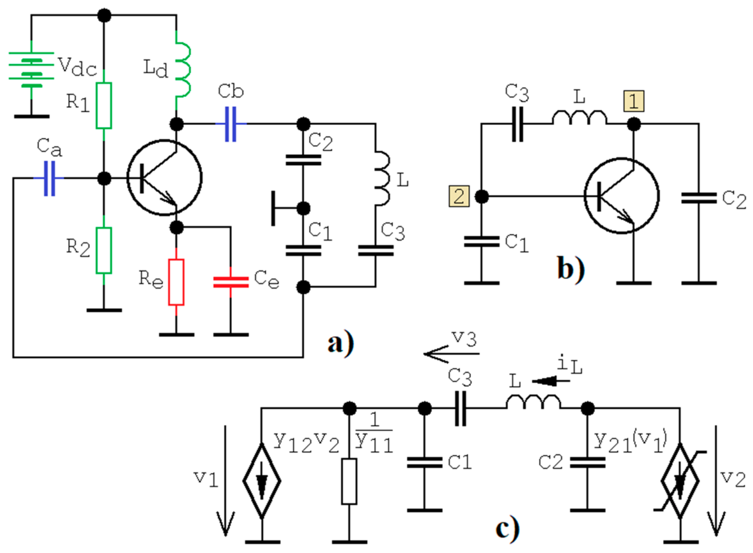
A Clapp oscillator can be understood as a slight modification of the famous Colpitts topology. The typical configuration of a Clapp oscillator is provided in Figure 1a. For the upcoming AC analysis, some circuit elements can be recognized as supporting and can be removed. To be more specific, green components serve to set up bias points, which is respected by the numerical values of admittance parameters. The blue color marks coupling capacitors and, due to the large values, can be substituted by the short circuit. Finally, the red color denotes a subcircuit dedicated for bias point temperature stabilization. After removing all colored elements, the Clapp oscillator simplifies into the network depicted in Figure 1b. Obviously, it is a fourth-order autonomous dynamical system and can be understood as a closed loop of a fourth-order trans-resistance filter and trans-conductance amplifier with a frequency-independent amplification. Using the notion of the Laplace transform and matrix method of unknown nodal voltages, the network function for the mentioned filter can be derived easily. By adopting node markings as indicated in the schematic, the admittance matrix can be expressed as

$$Y\left(s\right)=\left(\begin{array}{cc}{y}_{22}+s{C}_2+\tilde{Y}& -\tilde{Y}\\ -\tilde{Y}& y_{11}+s{C}_1+\tilde{Y}\end{array}\right) , \tilde{Y}\left(s\right)=\frac{s{C}_3}{s^2{C}_{3}L+1} ,$$

(1)

where s represents a complex frequency. Then, accordingly to Cramer´s rule, the trans-resistance of a passive ladder filter can be calculated symbolically as

$$K\left(s\right)=-\frac{v_{BE}}{i_C}=\frac{{\Delta }_{1,2}}{\Delta }=-\frac{s{C}_3}{{{\displaystyle \sum }}_{k=0}^4{a}_k{s}^k} ,$$

(2)

where Δ is the determinant of the admittance matrix, Δ_j,k is the determinant of the admittance matrix after removing the j-th row and k-th column, v_BE is the base-emitter voltage, i_C is the collector current of bipolar transistor, and the denominator coefficients are

$$\begin{gathered} a_4=C_1{C}_2{C}_{3}L, a_3=C_{3}L\left(C_2{y}_{11}+C_1{y}_{22}\right), a_2=C_1{C}_2+C_1{C}_3+C_2{C}_3+ \\ +C_3{y}_{11}{y}_{22}L, a_1=y_{11}\left(C_2+C_3\right)+y_{22}\left(C_1+C_3\right), a_0=y_{11}{y}_{22}, \end{gathered}$$

(3)

where y₁₁ and y₂₂ are the input and output admittance of the used bipolar transistor, respectively. Now, assume that the output admittance of a generalized transistor is zero ($y_{22}=0$), i.e., acts as the ideal current source. By combining network function (2) with parameters (3) and the trans-conductance nature of the bipolar transistor, $i_C=y_{21}{v}_{BE}$, we can obtain the characteristic equation of the Clapp oscillator

$$C_1{C}_2{C}_{3}L·s^3+y_{11}{C}_2{C}_{3}L·s^2+\left(C_1{C}_2+C_1{C}_3+C_2{C}_3\right)·s+y_{11}\left(C_2+C_3\right)+y_{21}·C_3=0,$$

(4)

In common situations, grounded capacitors are equivalent; C = C₁ = C₂. In this case, the condition for stable oscillation and associated oscillation frequency in Hz can be derived easily as

$$y_{21}=y_{11}, f_{osc}=\frac{1}{2\pi \sqrt{\frac{L}{\frac{2}{C}+\frac{1}{C_3}}}},$$

(5)

A substitution of the arbitrarily biased bipolar transistor with the so-called generalized bipolar transistor (GBT) is suggested in paper [22]. A subsequent analysis of a single-stage amplifier revealed the fact that several robust chaotic attractors can be observed even if this circuit is considered isolated, i.e., without an input driving signal. However, GBT needs to exhibit at least a small linear backward trans-conductance. This restriction is expected in electronic systems that contain neither local nor global feedback, i.e., very basic structures of amplifiers. The necessity to include backward trans-conductance to each GBT is also stated in paper [23], where a two-stage amplifier having a GBT and both resonant and resistive loads was analyzed. Four degrees of freedom allow for the existence of hyperchaotic self-oscillations.

Most low-frequency practical sinusoidal oscillators are composed by a closed loop of two blocks: an inverting or noninverting amplifier (constant phase shift 180° or 0°) and the passive ladder two-port feedback with frequency-dependent phase shifts. This passive two-port exhibits ±180° or 0° phase shift for the unique oscillation frequency. A high phase change around oscillation frequency contributes to an increased frequency stability. On the other hand, typical harmonic oscillators designed for high-frequency bands are based on parallel inductor–capacitor tanks where losses are compensated by the negative resistor.

A mathematical model that describes the Clapp oscillator with a nonlinear model of the bipolar transistor (with output admittance removed) can be expressed accordingly to Figure 1c as

$$\begin{gathered} C_1\frac{d{v}_1}{dt}=-y_{11}·v_1-y_{12}·v_2+i_L, C_2\frac{d{v}_2}{dt}=-y_{21}\left(v_1\right)-i_L, \\ {C}_3\frac{d{v}_3}{dt}=i_L, L\frac{d{i}_L}{dt}=v_2-v_1-v_3. \end{gathered}$$

(6)

where the state vector becomes x = (v₁ v₂ v₃ i_L)^T. The nonlinear forward trans-conductance can be an odd-symmetrical cubic polynomial function of the form

$$y_{21}\left(v_1\right)=a·v_1^3+b·v_1$$

(7)

which is saturation-type function. To get close to the standard operational regime of Clapp oscillators, relations a < 0 and b > 0 will be respected. Further in the text, we denote the Clapp oscillator having this polynomial type of transistor model Case I. Similarly, Case II will have a three-segment PWL approximation of forward trans-conductance, that is,

$$y_{21}\left(v_1\right)=a·v_1+\frac{1}{2}·\left(b-a\right)·\left(\left|v_1+1\right|-\left|v_1-1\right|\right),$$

(8)

where a and b are slopes of the PWL curve in the outer and inner segment of the function, respectively. Since the PWL function (5) approximates a cubic polynomial (7), we have parameters a < 0 and b > 0. Therefore, the state space is divided into three linear regions separated by two parallel planes v₁= ±1 V. The PWL function (8) is odd-symmetrical with respect to the origin. Note that breakpoints are considered fixed.

2.1. Clapp Oscillator, Case I

A dynamical system (6) with function (7) has a symmetrical vector field with respect to the origin and possesses three fixed points placed on the line, namely

$$x_1^{eq}=\left(\begin{array}{c}0\\ 0\\ 0\\ 0\end{array}\right), x_{2,3}^{eq}=\pm \sqrt{-\frac{b}{a}}·\left(\begin{array}{c}1\\ -\frac{y_{11}}{y_{12}}\\ -\frac{y_{11}}{y_{12}}-1\\ 0\end{array}\right).$$

(9)

We will look after the self-excited chaotic attractor driven by the equilibrium point located at the origin of the state space. Because of this, an origin should be a hyperbolic unstable fixed point, and we will prefer a saddle-focus local geometry characterized by at least single one-dimensional stable manifold. Eigenvalues that determine local dynamical movement near this equilibrium point are roots of the following characteristic polynomial:

$${\lambda }^4+y_{11}·{\lambda }^3+\left(3-b·y_{12}\right)·{\lambda }^2+\left(b+2·y_{11}+y_{12}\right)·\lambda -b·y_{12}=0.$$

(10)

A continuation with the symbolic evaluation of individual roots leads to very complicated formulas without further usage. The optimization discussed in the next section works with the numerical calculation of eigenvalues, calculated using Equation (10).

2.2. Clapp Oscillator, Case II

Analogically to Clapp oscillator, Case I, equilibrium points are all real solutions of the nonlinear problem dx/dt = 0. A straightforward analysis yields the following positions of three fixed points placed on a line, one in each region of the state space, namely,

$$x_1^{eq}=\left(\begin{array}{c}0\\ 0\\ 0\\ 0\end{array}\right), x_{2,3}^{eq}=\pm \frac{a-b}{a}\left(\begin{array}{c}1\\ -\frac{y_{11}}{y_{12}}\\ -\frac{y_{11}}{y_{12}}-1\\ 0\end{array}\right).$$

(11)

Since both addressed cases of the Clapp oscillator had the same derivative of the forward trans-conductance around zero, characteristic polynomial has the same form as (10). The roots of this polynomial were calculated numerically in each step of the optimization routine. Thus, further symbolic evaluation does not lead to useful results.

3. Numerical Results

Having a dimensionless mathematical model, the spectrum of LEs can be used to distinguish between different types of dynamical behavior. If the largest LE is significantly positive while the second in order converges to zero, system motion can be coined as chaotic. Even more interesting is the case with two distinguishable positive LEs, since it implies hyperchaotic behavior. In fact, the number of positive LEs represents the number of dimensions in which neighborhood state trajectories are separated on average. For each calculation of the fitness function, both initial conditions and sets of sought system parameters can serve as routine input variables.

Let us describe a three-step optimization approach developed and adopted in this paper in more detail. To reveal a self-excited attractor, a set of the initial conditions can be spread about the relevant equilibria. In our case, it is a fixed point located at the origin of the state space. Despite the variation of system parameters during optimization, this fixed point should remain unstable. Thus, combinations of system parameters that lead to the fixed-point full stabilization can be removed from our further considerations, preferably before the most time-consuming final step, the numerical calculation of the LE spectrum. Since parameter regions that are characterized by a system´s sensitivity dependance on initial conditions are often surrounded by an unbounded solution, the second step is to ensure that the ω-limit set is bounded. This can be performed via the inside-the-hypercube rule.

Without losing the chance to observe chaotic or hyperchaotic behavior, normalized values of all accumulation elements can be kept in unity. Backward trans-conductance, $y_{12}$, is kept low with respect to the rest of admittance parameters, $y_{11}, b$, to get close enough to the common operational state. Therefore, the hyperspace of system parameters dedicated for searching becomes four dimensional only. An objective function is aimed to discover “the most hyperchaotic” kind of dynamical motion of the investigated system. Thus, both the first- and second-largest LE needs to be maximized such that the Kaplan–Yorke dimension (KYD) will be maximal as well.

Of course, the existence of the so-called hidden attractors within dynamics of analyzed systems, either normal or strange, is not answered by the proposed optimization routine. Different methods on how to find such limit sets can be found in various papers [24,25]. From a practical application point of view, the investigation of attractors associated with a fixed point at the origin make more sense. This equilibrium exists even in the original non-chaotic Clapp oscillator. For this system, neighborhood of state space origin usually serves as start-up to produce sinusoidal oscillations.

3.1. Numerical Study of Case I

Using the search-for-chaos algorithm described in the previous paragraph, numerical values of the remaining system parameters can be chosen as

$$y_{11}=0.905 S, y_{12}=0.076 S, a=-1 A^3{V}^{-1}, b=4.82 S.$$

(12)

For these values, eigenvalues associated with the origin form a local vector field geometry that is composed of a three-dimensional unstable and one-dimensional stable manifold, namely

$$R^4\in R_{unstable}^2\oplus R_{unstable}^1\oplus R_{stable}^1 , {\lambda }_{1,2}=0.38\pm j1.96 , {\lambda }_3=0.052 , {\lambda }_4=-1.715.$$

(13)

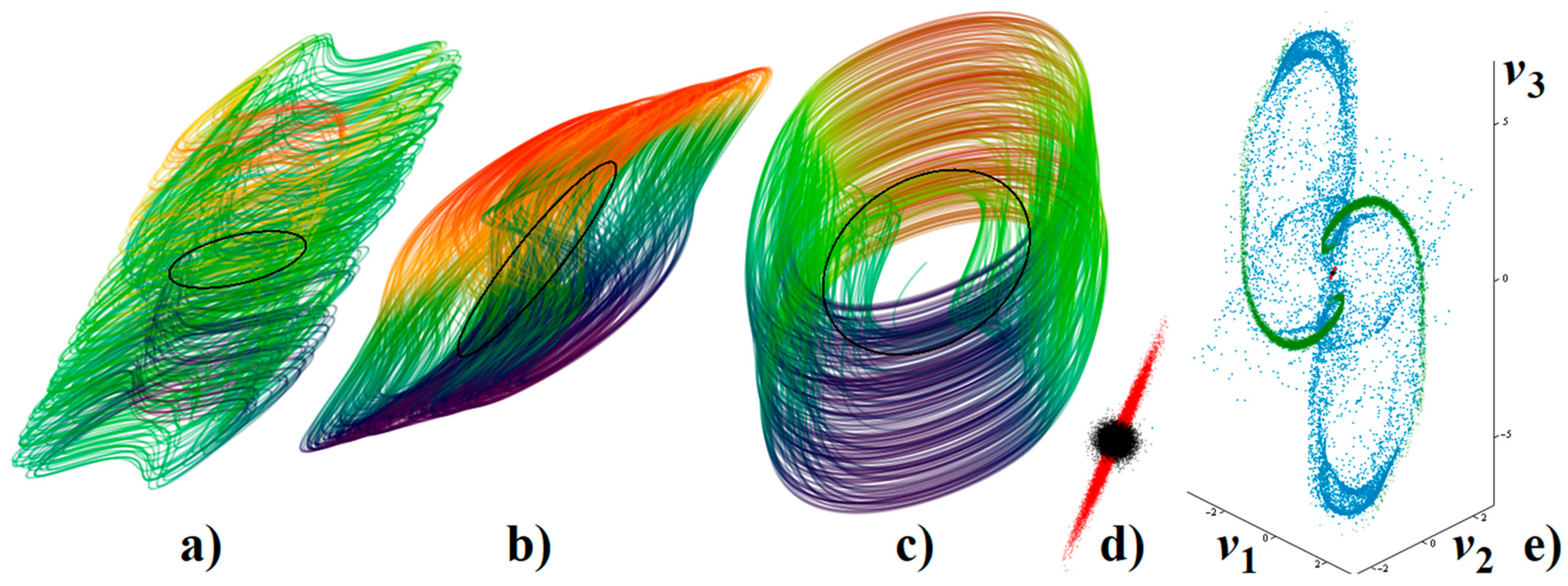
The choice of internal system parameters (12) together with a set of the initial conditions $x_0={\left(\begin{array}{cccc}0.1& 0& 0& 0\end{array}\right)}^{\mathrm{T}}$ lead to the strange attractor depicted in Figure 2a–c. In the same plots, the black circle shows the location of the limit cycle generated by a non-chaotic Clapp oscillator for the set of initial conditions $x_0={\left(\begin{array}{cccc}0& 0& 0& 4\end{array}\right)}^{\mathrm{T}}$. The forward trans-conductance of GBT becomes $y_{21}\left(v_1\right)=y_{11}\Delta v_1$, i.e., it has been linearized. Additionally, the backward trans-conductance of GBT has been removed, as typical for the quasi-linear analysis of a sinusoidal Clapp oscillator. Of course, the size and location of this limit cycle in the phase space depends on the choice of initial conditions. Figure 2d,e demonstrate the sensitivity of the system solution to tiny uncertainties in the initial conditions. There, black dots represent 10⁴ randomly generated initial conditions with a normal distribution and standard deviation 10⁻². Then, the final states after 1 s (red points), 10 s (green points), and 50 s (blue dots) are stored and visualized. Note that the analyzed dynamical system clearly exhibits sensitivity to small deviations of the initial conditions.

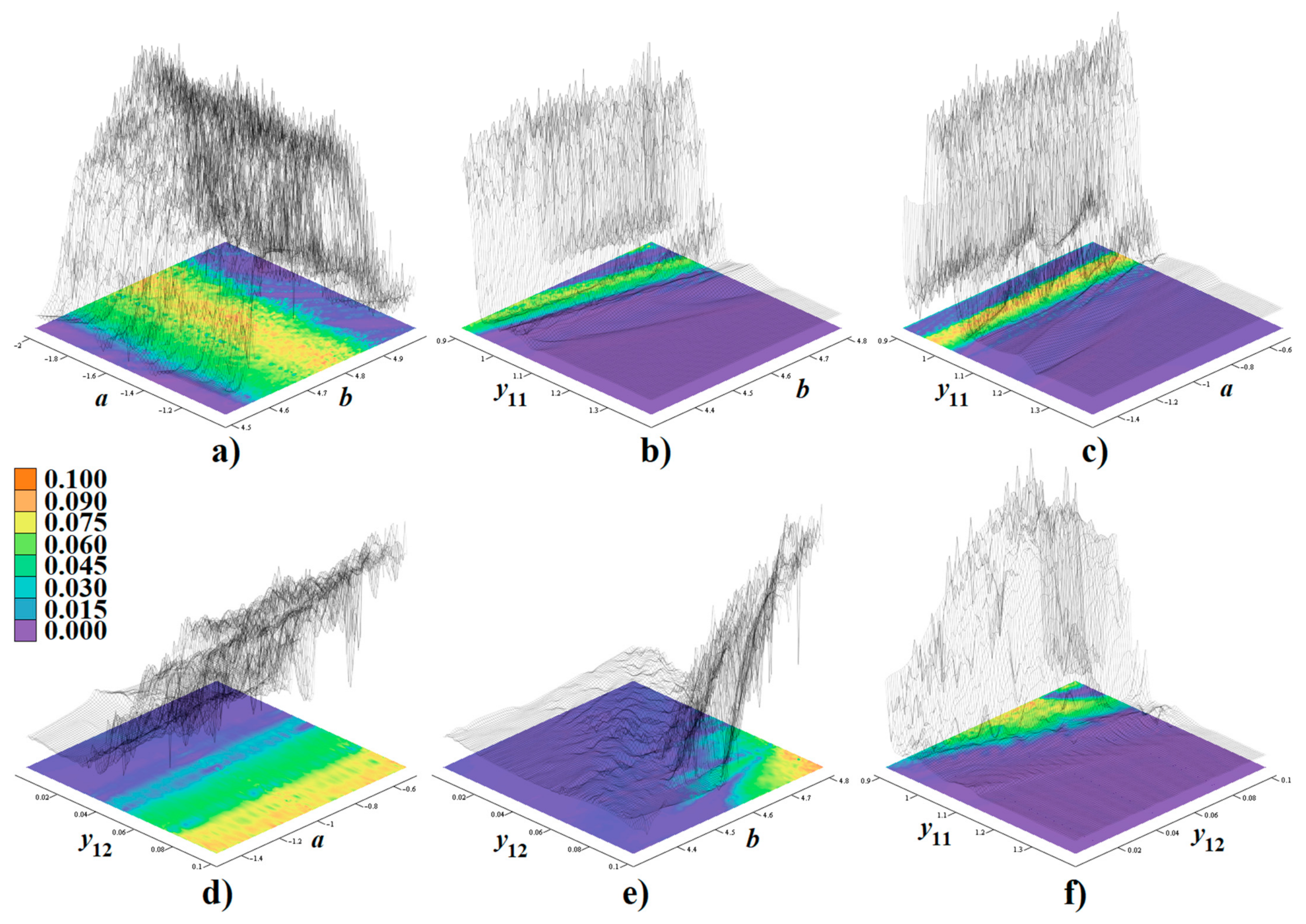
Figure 3 demonstrates a calculation of the largest LE in the fourth-dimensional hyperspace of internal parameters of the Clapp oscillator. To perform this task, a well-established algorithm that utilizes Gram–Smith orthogonalization described in book chapter [26] has been adopted. It should be noted that only a very small region is addressed, an interesting area where the qualitative change in system behavior becomes visible. A legend that provides the numerical value of the largest LE is also provided. For these calculations, initial conditions were chosen in the vicinity of the state space origin. Note that regions of strong chaos marked by the orange color are surrounded by the limit cycle solution (blue color). All these plots are high-resolution, with parameter step 10⁻², final time 1000 s, and time step 10 ms. For Figure 2 and Figure 3, parameters of the chosen fourth-order Runge–Kutta (RK) integration routine are set such that the stability of this numerical method is preserved. The RK method belongs to the most preferable integration algorithms for chaotic dynamical systems due to its high accuracy [27]. The RK method with fixed step size has been preferred over various RK methods with adaptive step sizes. Specifically, the size of the step was chosen significantly lower than the smallest exponential growth ratio that characterizes any existing unstable fixed point. Both the RK with fixed and adaptive step sizes belong to the build-in algorithms available in the Mathcad program (represented by function rkfixed and rkadapt, respectively). This piece of software was utilized for numerical integration and the graphical presentation of state trajectories.

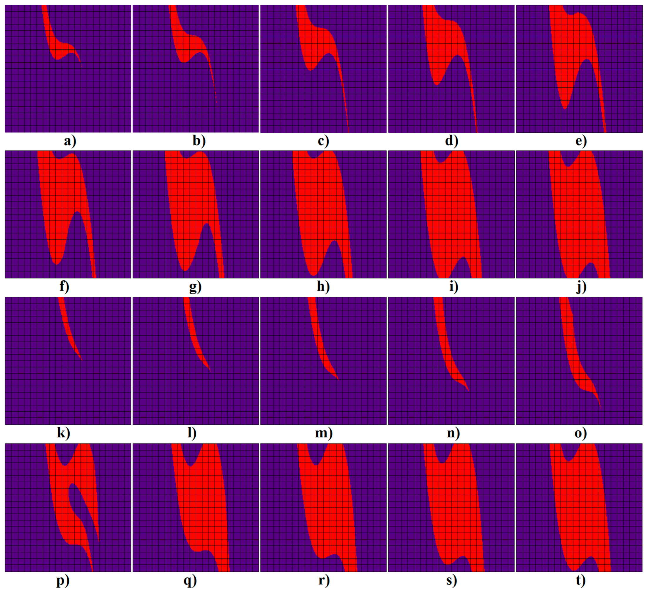
Figure 4 is a graphical visualization of basins of attraction for a generated strange attractor. In these plots, red denotes the set of initial conditions that end in a chaotic attractor, magenta represents areas that result in an unbounded solution. The step of the initial conditions adopted for these calculations was uniformly chosen as 10 mV; the grid is v₁ ∈ (−10, 10) V and v₂ ∈ (−10, 10) V.

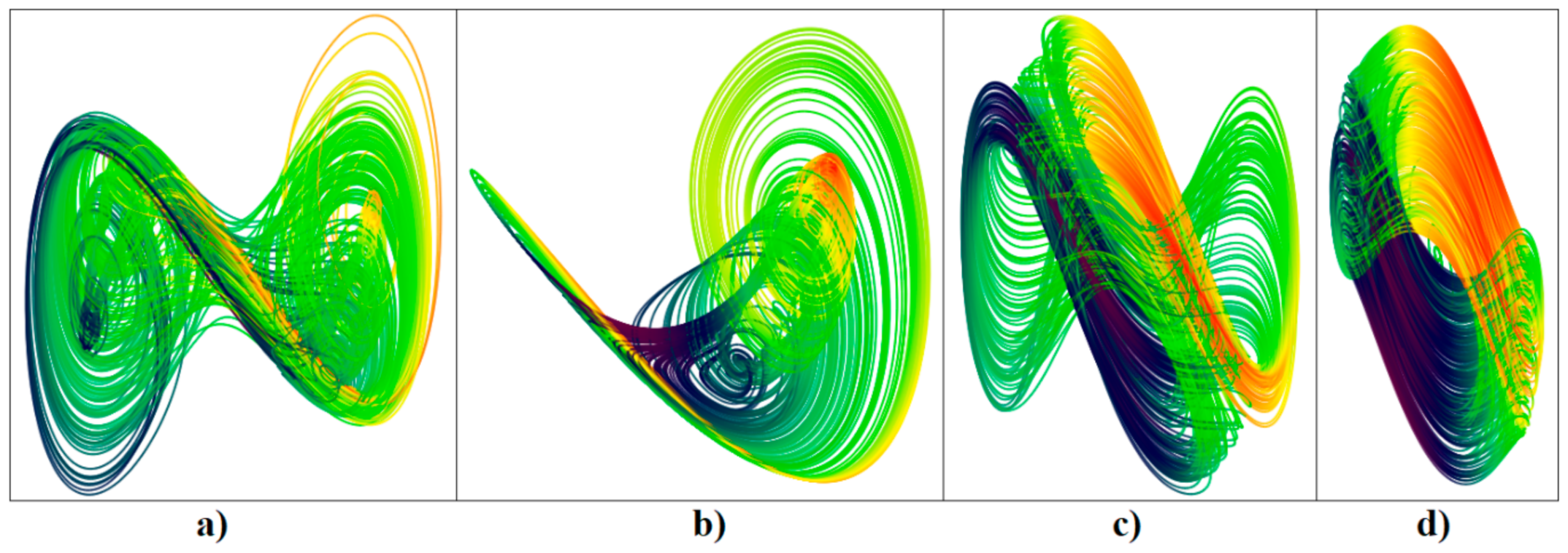
Figure 5 shows other interestingly shaped strange attractors discovered by the search-for-chaos routine (sizes of all attractors are comparable to the attractor in Figure 2). The initial conditions for Figure 5a,c were $x_0={\left(\begin{array}{cccc}0.1& 0& 0& 0\end{array}\right)}^{\mathrm{T}}$, and the numerical value of parameter a = −1 A³V⁻¹ was kept for all plots. Individual numerically integrated trajectories have a rainbow color scale that represents growing inductor current. The final time was chosen as 1000 s and time step 10 ms. Note that the geometrical structures of the chaotic attractor given in Figure 5a,b are geometrically similar to the famous double-scroll and single-scroll, respectively, although this strange attractor is formed within the state space having four dimensions.

3.2. Numerical Analysis of Case II

In this subsection, Case II of an investigated dynamical system (6) will be addressed. By using the search-for-chaos numerical algorithm mentioned above, a discovered parameter set with locally maximized chaotic motion is

$$y_{11}=1 \mathrm{S}, y_{12}=0.1 \mathrm{S}, a=-9.98 \mathrm{S}, b=3.78 \mathrm{S}.$$

(14)

Eigenvalues associated with the origin forms local vector field geometry that is composed by a three-dimensional unstable and one-dimensional stable manifold, namely

$$R^4\in R_{unstable}^2\oplus R_{unstable}^1\oplus R_{stable}^1, {\lambda }_{1,2}=0.295\pm j1.89, {\lambda }_3=0.062, {\lambda }_4=-1.652.$$

(15)

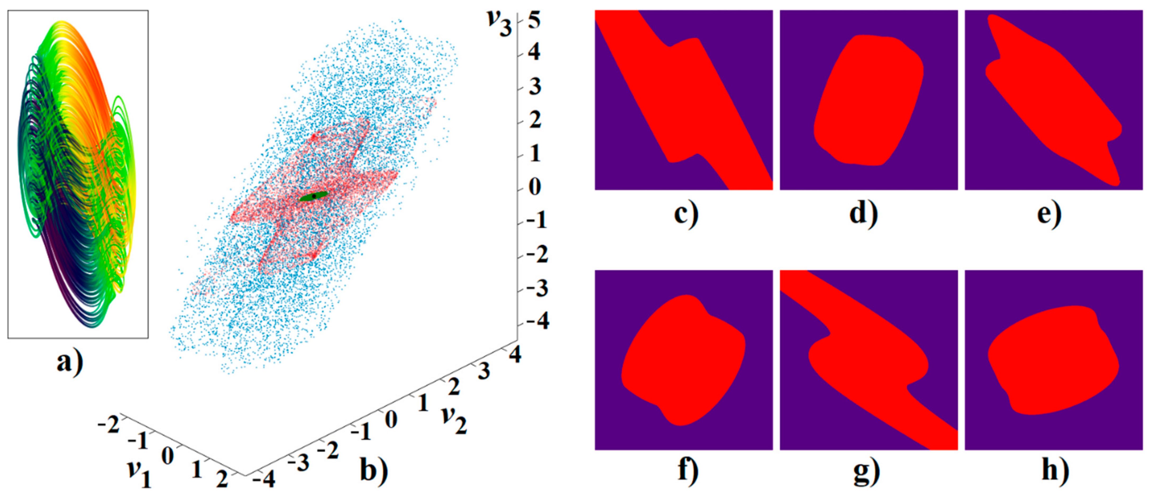
As expected, the geometrical formation of the vector field close to the state space origin is like the Clapp oscillator, Case I. Numerical analysis of dynamical system (6) with PWL functionality (8) and parameter set (14) is provided by means of Figure 6. Besides the typical strange attractor, this figure contains a subplot that demonstrates the sensitivity of the system solution to a group of 10⁴ initial conditions generated using normal distribution with standard deviation 10⁻² around the origin (black dots). Then, final states are visualized after 1 s (green dots), 20 s (red dots), and 50 s (blue states) of time evolution (integrated using uniform time step 10 ms). The short time evolution shows directions of the fastest dynamical flow local to the origin of the state space. After a time evolution of 50 s, the final states fill a subset of 4D state space with a non-integer geometrical dimension. Figure 6c–h also shows calculated basins of attraction for this strange attractor (red color) vs. unbounded solution (purple color). Of course, there are always third types of solutions, fixed points (equilibria). Axis ranges for the initial states were chosen as v₁⁰ ∈ (−7, 7) V, v₂⁰ ∈ (−15, 15) V, v₃⁰ ∈ (−15, 15) V, and i_L⁰ ∈ (−15, 15) A. It should be noted that the attraction set forms a compact volume that surrounds the equilibrium point located at the state space origin.

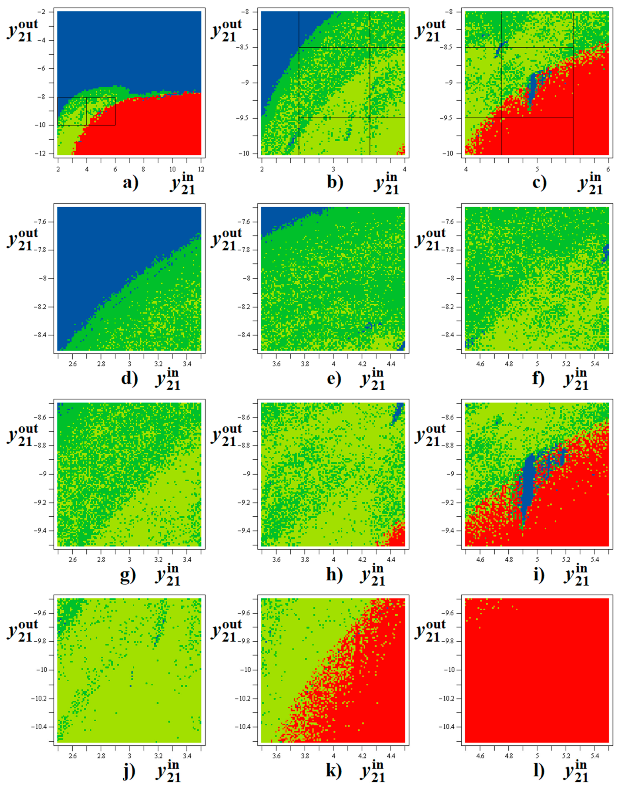
Figure 7 demonstrates different types of dynamical behavior excited by the unstable fixed point located at the origin of the state space. The dynamical flow is quantified with respect to both parameters of PWL functionality (8) where, for better understanding, the linear slopes in the outer and inner segments are denoted $y_{21}^{out}\equiv \mathrm{a}, y_{21}^{in}\equiv \mathrm{b}$, respectively. Each figure contains 101 × 101 = 10201 points calculated for the final time, 1000 s, and time step, 10 ms. Note that the individual areas are riddled and immersed into each other. Different types of dynamical motions are distinguished by adopting the concept of LE and, after a quantification process, re-verified by random repeated numerical integration.

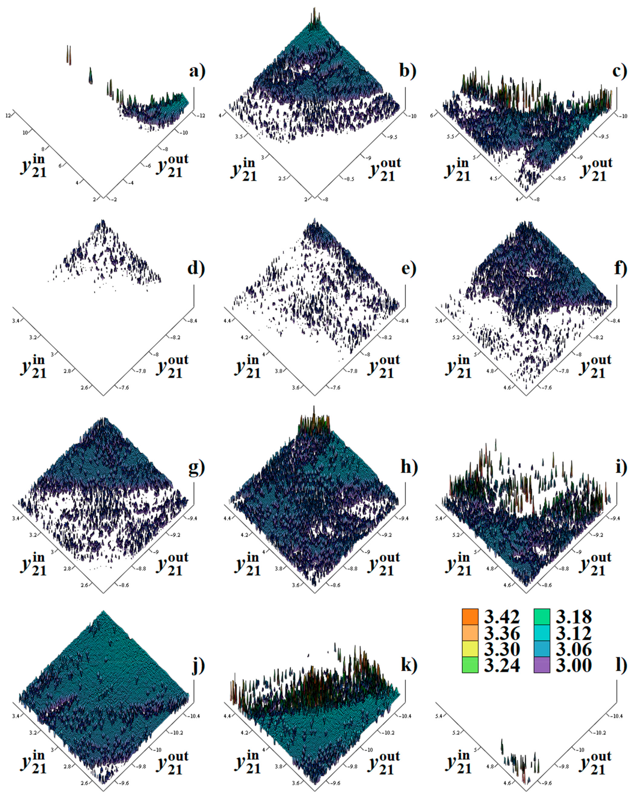
Figure 8 represents rainbow-scaled surface plots of KYD plotted with respect to the parameters of the PWL function (associated with the nonlinear forward trans-conductance y₂₁). The missing surface means that the solution excited by the unstable equilibrium located at zero suddenly becomes unbounded. The analyzed fourth-order dynamical system exhibits hyperchaotic movement in a wide parameter range, the strongest two-dimensional state space expansion along the trajectory (in average) borders with the unbounded solution.

Now, this is the right moment to raise an interesting question about the transition process between the chaotic and hyperchaotic behavior of the analyzed dynamical system. Such a problem has been already addressed in several papers. Properties of attractors near transition points (in the sense of the smooth change of a bifurcation parameter) are discussed in work [28]. There, it is stated that the chaos–hyperchaos transition is caused by one of the following two reasons: (1). changing the sign of the real part of some real or complex conjugated eigenvalues, i.e., change of local vector field geometry associated with fixed point that affects shape of generated strange attractor. Thus, each bifurcation parameter that causes such a change can be easily recognized, along with a range of its values worthy to be investigated. (2). The shape of the generated strange attractor starts to be influenced by the vector field geometry associated with fixed points located outside the attractor. This is a reasonable assumption especially in the case of moving the mentioned equilibrium toward an observed attractor or increasing size of attractor (as bifurcation parameter changes).

Note that both rules are more likely hypotheses than rigorous statements expressed by analytical formulas. A numerical study of chaos–hyperchaos transitions in a fourth-dimensional modified Rossler system is provided in paper [29]. There, up to eight mathematical models are briefly analyzed with respect to the information dimension and prediction time. Each system possesses polynomial a vector field similar to our Clapp oscillator, Case I. Let us try to follow up the procedure suggested by the authors. If we fix numerical values (12), we obtain two additional fixed points, $x_{2,3}^{eq}=\pm {\left(\begin{array}{cccc}2.195& -26.143& -28.339& 0\end{array}\right)}^{\mathrm{T}}$, which are located far away from strange the attractor. It can be shown that both (10) and the characteristic polynomial associated with outer fixed points depend on the parameter b rather than the cubic term a. If we change this parameter in the investigated range, b ∈ (3, 5) S, there are no changes in the signs of the real parts of eigenvalues associated with any equilibrium point. However, in the mentioned parameter range, the solution experiences limit cycles and chaotic as well as hyperchaotic motion with a very low prediction time, only about 5.68. As can be also noticed in this range, the size of attractor remains almost the same, and outer fixed points are still far away from the attractor. Thus, some other rule probably plays a crucial role in the process of chaos–hyperchaos transitions.

The same analysis can be performed for a Clapp oscillator with PWL forward trans-conductance. If we adopt numerical values (14), the positions of the outer fixed points will be $x_{2,3}^{eq}=\pm {\left(\begin{array}{cccc}1.379& -13.788& -15.166& 0\end{array}\right)}^{\mathrm{T}}$. These locations are far away from the attractor. However, because of attractor boundedness, the trajectory repeatedly leaves the inner segment of the vector field, stays in the outer segment for a while, and then is pushed again toward the inner segment. Thus, the vector field geometry associated with the outer fixed points is important. Firstly, let us study changes in the signs of eigenvalues associated with a fixed point located at the origin. In such a case, parameter b becomes important, and the investigated range can be extended to b ∈ (1, 10) S. However, there are no changes in the signs of the roots of the characteristic polynomial. To calculate eigenvalues associated with the outer fixed point, parameter b in characteristic equation (10) should be replaced by parameter a with extended range, a ∈ (−10, −1) S. In the interval a = −10 S up to a = −2 S, the geometry of the vector field in the outer segment is $R^4\in R_{unstable}^2\oplus R_{unstable}^2$; then it changes into $R^4\in R_{stable}^2\oplus R_{stable}^2$, and for a ≥ −1 S it changes again into $R^4\in R_{stable}^2\oplus R_{stable}^1\oplus R_{stable}^1$. Note that the increasing of parameter a cause the outer fixed points to move away from the attractor (its size does not significantly change). The mentioned bifurcation points a ≈ −2 S and a ≈ −1 S do not represent values where dynamical motion is chaotic or hyperchaotic. Therefore, the real cause of chaos–hyperchaos transition process still remains a mystery.

Other numerical approaches can be utilized to study mechanisms behind a chaos–hyperchaos transition. For further reading, the interesting paper [30] can be recommended. There, the correlation dimension and recurrence plots are visualized and compared to distinguish between chaotic and hyperchaotic regimes. It should be pointed out that the Murali–Lakshmanan–Chua circuit driven by the sinusoidal signal is considered in this paper, i.e., the nature of analyzed dynamical systems is different from autonomous systems addressed in this work.

4. Experimental Results

The construction and experimental verification through laboratory measurement generally belong to the presentation of a new chaotic dynamical system [31]. In an analog circuit design of a chaotic oscillator, very short time constants are usually adopted. This is also the case of each realization proposed in this paper. A pattern that settles down on an oscilloscope screen during measurement represents the true ω-limit set of the observed state attractor. Due to the natural smooth integration process of the accumulation elements, trivial fixed-point end-states or unbounded solutions cannot be misinterpreted with strange attractors. Because of these reasons, a true experimental confirmation of the existence of the strange attractors is indeed a good way how to prove that observed chaos is neither a long transient motion nor numerical artifact. Comprehensive review papers dealing with circuit synthesis tasks based on a set of ordinary differential equations include [32,33].

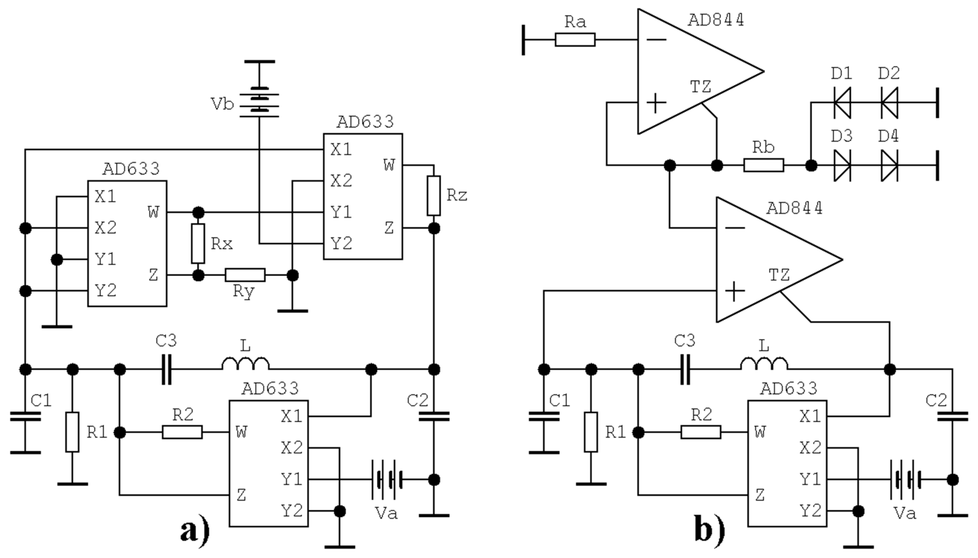
The circuit implementation of an analyzed dynamical system with polynomial nonlinearity is provided by means of Figure 9a. Describing a set of first-order ordinary differential equations can be expressed as

$$C_1\frac{d{v}_1}{dt}=-\frac{v_1}{R_1}-\frac{K·v_2·V_a}{R_2}+i_L, C_2\frac{d{v}_2}{dt}=\frac{K·v_1\left(v_1^2-V_b\right)}{R_z}-i_L, C_3\frac{d{v}_3}{dt}=i_L, L\frac{d{i}_L}{dt}=v_2-v_1-v_3,$$

(16)

where K = 0.1 is the internally trimmed transfer constant of used analog multiplier AD633. This circuit realization of the Clapp oscillator needs three AD633s, one connected as a voltage-controlled trans-admittance amplifier. External DC voltages V_a and V_b represent parameters y₁₂ and b, respectively; both can be used as the natural bifurcation parameters. Since impedance and frequency scaling factors can be arbitrary, we can use for example values 10³ and 10⁶. This choice leads to the following set of numerical values:

$$C_1=C_2=C_3=1 nF, L=1 mH, R_1=R_x=1 k\mathsf{\Omega }, R_2=1.3 k\mathsf{\Omega }, R_y=9 k\mathsf{\Omega }, R_z=100 \mathsf{\Omega }.$$

(17)

A suitable choice of resistors R_x and R_y, namely if equality R_y = 9⋅R_x holds, leads to the full compensation of the voltage scaling factor K of the first analog multiplier.

In the case of the Clapp oscillator with PWL functionality, the subcircuit that represents the linear part of the vector field is the same as for system (16); see Figure 9b. Therefore, the same impedance and frequency scaling factors can be chosen, i.e., 10³ and 10⁶. The complete set of ordinary differential equations for the circuit given in Figure 9b is

$$C_1\frac{d{v}_1}{dt}=-\frac{v_1}{R_1}-\frac{K·v_2·V_a}{R_2}+i_L, C_2\frac{d{v}_2}{dt}=-\frac{v_1}{R_a}+\frac{v_1}{R_b+2·R_d}-i_L, C_3\frac{d{v}_3}{dt}=i_L, L\frac{d{i}_L}{dt}=v_2-v_1-v_3,$$

(18)

where R_d is the differential resistance of diodes. This value is very low in the inner segment of the vector field (defined by voltage v₁ < 2⋅V_t) and very large (for voltage v₁ > 2⋅V_t), respectively, where V_t represents a threshold voltage of diode. For practical experiments, diodes BAT42 were utilized. The list of numerical values associated with passive circuit elements is

$$C_1=C_2=C_3=1 nF, L=1 mH, R_1=1 k\mathsf{\Omega }, R_2=1 k\mathsf{\Omega }, R_a=265 \mathsf{\Omega }, R_b=10 \mathsf{\Omega }).$$

(19)

The value of resistor R_b is a rough approximation, since the dynamic resistance of one (or several) forwardly biased diode is connected in series. Due to the chosen impedance norm 10³, the total power consumption of this realization of chaotic oscillator is significant (up to 1.5 W).

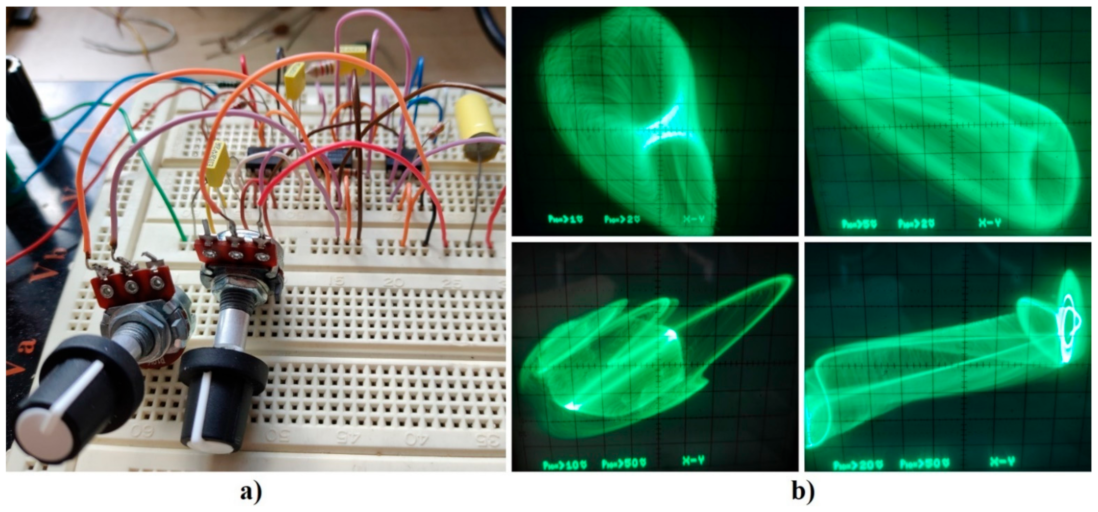
A few oscilloscope screenshots captured during the experimental verification of the designed Clapp oscillator, Case I (using bread board) are shown in Figure 10. Note that the external voltages can be used to change system behavior accordingly to Figure 3e, i.e., we can easily trace the route-to-chaos scenario in two parametric dimensions. A very good final agreement between theoretical shapes and practically observed strange attractors can be concluded.

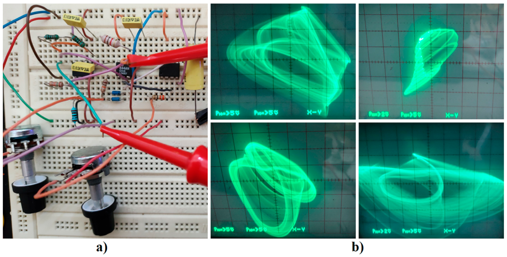
Figure 11 provides an experimental verification of the presence of chaotic regimes associated with the Clapp oscillator, Case II. A gallery of differently shaped strange attractors has been observed, just as in the numerical analysis.

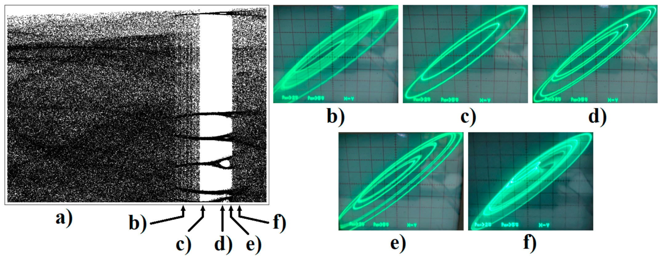
Figure 12 shows a one-dimensional bifurcation diagram calculated for the small steps of parameter b, i.e., the short variation of the external voltage V_b. For numerical calculation, the initial conditions were set to x₀ = (1, 0, 3, 0)^T, final time 10⁴ s, and time step 10 ms. The bifurcation diagram is plotted for planes defined as v₃ = 0 V, then the state variable v₁ is stored and visualized. Note that by changing V_b in a very narrow numerical range, we can trace the evolution of chaos via a period doubling the bifurcation sequence.

Note that both autonomous circuits given in Figure 9 are very simple and contain very few active elements. Moreover, a chaotic electronic system with a polynomial vector field was constructed by using only analog multipliers as active devices. Of course, this is not a new idea. The same approach can be found in much older papers, but it is still an up-to-date method, as evident from the recent brief study [34]. By adopting analog multipliers as trans-conductance cells, the final network topology is much simpler if compared with an analog computer concept. This will be evident also from the upcoming text.

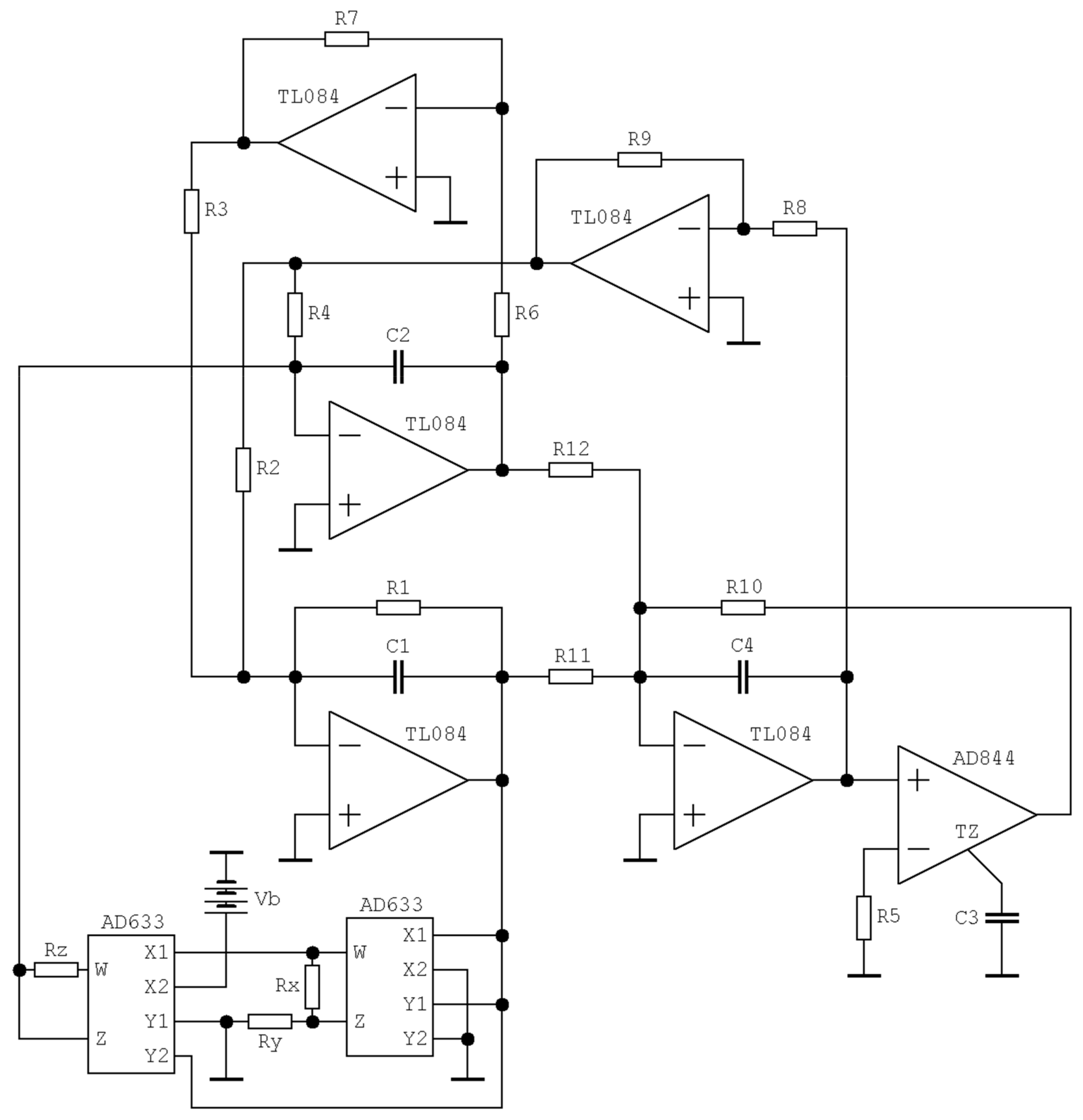
Figure 13 demonstrates an alternative circuitry realization of the chaotic Clapp oscillator based on the integrator block schematic. The network consists of three inverting and single non-inverting lossless integrators, two inverting amplifiers, and a trans-conductance mode nonlinear two-port with a cubic polynomial transfer function. Describing the set of differential equations, we have

$$C_1\frac{d{v}_1}{dt}=-\frac{v_1}{R_1}+\frac{R_7·v_2}{R_3·R_6}+\frac{R_9·v_4}{R_2·R_8}, C_2\frac{d{v}_2}{dt}=\frac{R_9·v_4}{R_4·R_8}-\frac{K·v_1\left(v_1^2-V_b\right)}{R_z}, C_3\frac{d{v}_3}{dt}=\frac{v_4}{R_5}, C_4\frac{d{v}_4}{dt}=-\frac{v_1}{R_{11}}-\frac{v_2}{R_{12}}-\frac{v_3}{R_{10}},$$

(20)

where the fundamental time constant of the oscillator can be chosen as τ = R⋅C = 10³⋅10–7 = 100 μs, and, consequently, numerical values of the passive circuit elements are the following:

$$\begin{gathered} C_1=C_2=C_3=C_4=100 nF, R_1=1.1 k\mathsf{\Omega }, R_2=R_4=R_5=R_{10}=R_{11}=R_{12}=1 k\mathsf{\Omega }, \\ {R}_6=R_7=R_8=R_9=10 k\mathsf{\Omega }, R_3=13 k\mathsf{\Omega }, R_x=1 k\mathsf{\Omega }, R_y=9 k\mathsf{\Omega }, \end{gathered}$$

(21)

where Ry = 9⋅R_x just to compensate the K = 0.1 voltage transfer constant of the first analog multiplier. The generated chaotic waveform can be frequency rescaled easily via the simultaneous change of all capacitors. Note that a linear transformation of the coordinates −v₂ → v₂ was adopted just to make the final circuit realization simpler.

5. Discussion

This paper demonstrates that the conventional structure of a Clapp oscillator can enter a chaotic steady state under two conditions: active element with weak local linear feedback and nonlinear transfer characteristics. These requirements are closely related to the common operational regime of the high-frequency sinusoidal oscillator having a bipolar transistor. Note that the model of GBT used as an active element is considered resistive, i.e., free of parasitic capacitances between individual terminals.

Speaking in the terms of numerical analysis, the generated strange attractors have been optimized from the viewpoint of the maximization of time domain unpredictability. The Clapp oscillator, Class I, had a largest LE of about 0.102 and KYD approximately equal to 3.126. Similarly, the Clapp oscillator, Class II, exhibited a largest LE of about 0.131 and maximal KYD close to value 3.41. The investigated dynamical system is invariant under the complete inversion of state coordinates. The circuit realization of chaotic oscillators was simple, with only three active elements. On the other hand, both final circuits turned out to be very sensitive to the exact values of passive circuit components.

6. Conclusions

This section will briefly discuss the discovery of the chaotic regime of the Clapp oscillator in a broader context, including the motivation to look after the non-conventional dynamic behavior of deterministic mathematical models.

If investigated analog functional blocks are commonly included in radio-frequency communication paths, it is highly desired to mark up all possible steady states and the conditions of their origin. Thus, research oriented toward searching-for-chaos is still up to date, although the utilized routine represents a brute force numerical approach [35]. The mentioned searching comprises calculations of a huge number of parametric combinations associated with an analyzed dynamical system, and this is allowed thanks to modern computational tools, in particular parallel processing in MATLAB using multi-core computers.

The Clapp oscillator, especially if treated as generally as possible, clearly belongs to standard functional subparts of complex electronic systems located on the transmitter as well as receiver side. There are three essential questions that should be asked at this time. Firstly: How close is (in the parameter sense) the common (known) and chaotic (unknown) operational state? Answer: In the case of a Clapp oscillator, it is rather close for the oscillator working at high frequency bands. However, the process of bipolar transistor unilaterization can significantly decrease the local linear feedback necessary for chaos evolution, causing chaos to disappear. Secondly: What are the main differences between mathematical models that describe the original and chaotic Clapp oscillator? Answer: Formally, these models are the same. The only difference is the nonlinear nature of the forward trans-conductance of an active two-port device. Third question: Does the nonlinear function used for chaos generation accurately model the real nature of the active element? Answer: For both Cases of the Clapp oscillator addressed in this paper, we used a saturation-type function with a positive slope of forward trans-conductance. This is indeed related to the real practical situation. The concrete shape, or more likely a size, of nonlinearity can be changed/adjusted via suitable rescaling.

This paper opens new possibilities for future investigation. For example, the so-called multi-stability and coexistence of several strange attractors within an analyzed dynamical system remains a mystery. Fans of fractional-order calculus can consider some accumulation circuit element of fractional order. An analysis of mathematical models modified in such a way can reveal new shapes of strange attractors [36]. Last but not least, the implementation of chaotic Clapp oscillators using an FPGA development kit can lead to interesting results.

Final remark: the circuit realization of the analyzed Clapp oscillator is closely related to the so-called Pierce oscillator, where the series connection of the inductor and capacitor in the feedback loop of a bipolar transistor is substituted by piezoelectric crystal. However, the shunt and series capacitor inside the equivalent circuit of a crystal element (for first paired series-parallel resonance) has completely different values and cannot be treated as equal. Moreover, the high quality factor of the resonator will filter out all frequency components except the fundamental harmonic. Considering all this, forcing the Pierce oscillator to behave chaotically probably requires pushing circuit parameters far away from the common operational regime and the mathematical model far away from physical reality.

References

- Matsumoto, T. A chaotic attractor from Chua´s circuit. IEEE Trans. Circuits Syst. 1984, 31, 1055–1058. [Google Scholar] [CrossRef]
- Zhong, G.-Q. Implementation of Chua´s circuit with cubic nonlinearity. IEEE Trans. Circuits Syst. I Fundam. Theory Appl. 1994, 41, 934–941. [Google Scholar] [CrossRef] [Green Version]
- Kennedy, M.P. Chaos in the Colpitts oscillator. IEEE Trans. Circuits Syst. I Fundam. Theory Appl. 1994, 41, 771–774. [Google Scholar] [CrossRef]
- Kennedy, M.P. On the relation between the chaotic Colpitts oscillator and Chua’s oscillator. IEEE Trans. Circuits Syst. I Fundam. Theory Appl. 1995, 42, 376–379. [Google Scholar] [CrossRef]
- Kvarda, P. Chaos in Hartley’s oscillator. Int. J. Bifurc. Chaos 2002, 12, 2229–2232. [Google Scholar]
- Morgul, O. Wien bridge based RC chaos generator. Electron. Lett. 1995, 31, 2058–2059. [Google Scholar] [CrossRef] [Green Version]
- Kilic, R.; Yildrim, F. A survey of Wien bridge-based chaotic oscillators: Design and experimental issues. Chaos Solitons Fractals 2008, 38, 1394–1410. [Google Scholar] [CrossRef]
- Elwakil, A.S.; Kennedy, M.P. Chaotic oscillators derived from sinusoidal oscillators based on the current feedback op amp. Analog. Integr. Circuits Signal Processing 2000, 24, 239–251. [Google Scholar] [CrossRef]
- Bernat, P.; Balaz, I. RC autonomous circuits with chaotic behavior. Radioengineering 2002, 11. [Google Scholar]
- Ogorzalek, M.J. Order and chaos in a third-order RC ladder network with nonlinear feedback. IEEE Trans. Circuits Syst. 1989, 36, 1221–1230. [Google Scholar] [CrossRef]
- Petrzela, J. Simple chaotic oscillator: From mathematical model to practical experiment. Radioengineering 2006, 15, 6–12. [Google Scholar]
- Petrzela, J.; Polak, L. Minimal realizations of autonomous chaotic oscillators based on trans-immittance filters. IEEE Access 2019, 7, 17561–17577. [Google Scholar] [CrossRef]
- Endo, T.; Chua, L.O. Chaos from phase-locked loops. IEEE Trans. Circuits Syst. 1988, 35, 987–1003. [Google Scholar] [CrossRef]
- Endo, T. A review of chaos and nonlinear dynamics in phase-locked loops. J. Frankl. Inst. 1994, 331, 859–902. [Google Scholar] [CrossRef]
- Fossas, E.; Olivar, G. Study of chaos in the buck converter. IEEE Trans. Circuits Syst. I Fundam. Theory Appl. 1996, 43, 13–25. [Google Scholar] [CrossRef] [Green Version]
- Dean, J. Chaos in a current-mode controlled boost DC-DC converter. IEEE Trans. Circuits Syst. I Fundam. Theory Appl. 1992, 39, 680–683. [Google Scholar] [CrossRef]
- Tse, C.K.; Chan, W.C.Y. Chaos from a current-programmed cuk converter. Int. J. Circuit Theory Appl. 1995, 23, 217–225. [Google Scholar] [CrossRef]
- Di Bernardo, M.; Garefalo, F.; Glielmo, L.; Vasca, F. Switching bifurcations, and chaos in DC/DC converters. IEEE Trans. Circuits Syst. I: Fundam. Theory Appl. 1998, 45, 133–141. [Google Scholar] [CrossRef]
- Hamill, D.C.; Jeffries, D.J. Subharmonics and chaos in a controlled switched-mode power converter. IEEE Trans. Circuits Syst. 1988, 35, 1059–1061. [Google Scholar] [CrossRef]
- Tse, C.K. Flip bifurcation and chaos in three-state boost switching regulators. IEEE Trans. Circuits Syst. I Fundam. Theory Appl. 1994, 41, 16–23. [Google Scholar] [CrossRef]
- Rodriguez-Vazquez, A.; Huertas, J.; Chua, L.O. Chaos in switched-capacitor circuit. IEEE Trans. Circuits Syst. 1988, 32, 1083–1085. [Google Scholar] [CrossRef]
- Petrzela, J. Evidence of strange attractor in class C amplifier with single bipolar transistor: Polynomial and piecewise-linear case. Entropy 2021, 23, 175. [Google Scholar] [CrossRef] [PubMed]
- Petrzela, J. Hyperchaotic self-oscillations of two-stage class C amplifier with generalized transistors. IEEE Access 2021, 9, 62182–62194. [Google Scholar] [CrossRef]
- Leonov, G.A.; Kuznetsov, N.V. Hidden attractors in dynamical systems. Form hidden oscillations in Hilbert-Kolmogorov, Aizerman, and Kalman problems to hidden chaotic attractor in Chua circuits. Int. J. Bifurc. Chaos 2013, 23, 1330002. [Google Scholar] [CrossRef] [Green Version]
- Dudkowski, D.; Jafari, S.; Kapitaniak, T.; Kuznetsov, N.V.; Leonov, G.A.; Prasad, A. Hidden attractors in dynamical systems. Phys. Rep. 2016, 637, 1–50. [Google Scholar] [CrossRef]
- Sprott, J.C. Chaos and Time Series Analysis; Oxford University Press: Oxford, UK, 2003; pp. 116–117. [Google Scholar]
- Valencia-Ponce, M.A.; Tlelo-Cuautle, E.; De la Fraga, L.G. Estimating the highest time-step in numerical methods to enhance the optimization of chaotic oscillators. Mathematics 2021, 9, 1938. [Google Scholar] [CrossRef]
- Kapitaniak, T.; Thylwe, K.-E.; Cohen, I.; Wojewoda, J. Chaos-hyperchaos transition. Chaos Solitons Fractals 1995, 5, 2003–2011. [Google Scholar] [CrossRef]
- Nikolov, S.; Clodong, S. Hyperchaos-chaos-hyperchaos transition in modified Rossler systems. Chaos Solitons Fractals 2006, 28, 252–263. [Google Scholar] [CrossRef]
- Manimehan, I.; Paul Asir, M.; Philominathan, P. Chaotic and hyperchaotic dynamics of a modified Murali-Lakshmanan-Chua circuit. J. Comput. Nonlinear Dyn. 2019, 14, 051001. [Google Scholar] [CrossRef]
- Sprott, J.C. A proposed standard for the publication of new chaotic systems. Int. J. Bifurc. Chaos 2011, 21, 2391–2394. [Google Scholar] [CrossRef] [Green Version]
- Itoh, M. Synthesis of electronic circuits for simulating nonlinear dynamics. Int. J. Bifurc. Chaos 2001, 11, 605–653. [Google Scholar] [CrossRef]
- Petrzela, J.; Gotthans, T.; Guzan, M. Current-mode network structures dedicated for simulation of dynamical systems with plane continuum of equilibrium. J. Circuits Syst. Comput. 2018, 27, 1830004. [Google Scholar] [CrossRef]
- Wu, J.; Li, C.H.; Ma, X.; Lei, T.; Chen, G. Simplification of chaotic circuits with quadratic nonlinearity. IEEE Trans. Circuits Syst. II Express Briefs 2022, 69, 1837–1841. [Google Scholar] [CrossRef]
- Keuninckx, L.; Van der Sande, G.; Danckaert, J. Simple two-transistor single-supply resistor-capacitor chaotic oscillator. IEEE Trans. Circuits Syst. II: Express Briefs 2015, 62, 891–895. [Google Scholar] [CrossRef]
- Tlelo-Cuautle, E.; De La Fraga, L.G.; Guillen-Fernandez, O.; Silva-Juarez, A. Optimization of Integer/Fractional Order Chaotic Systems by Metaheuristics and Their Electronic Realization, 1st ed.; Taylor & Francis Group: London, UK, 2021; p. 266. [Google Scholar]
Figure 1.
Clapp oscillator: (a) standard complete topology including biasing circuits, (b) simplified structure for quasilinear analysis, and (c) network with nonlinear model of bipolar transistor.
Figure 2.
Typical strange attractor generated by transistor-based Clapp oscillator visualized in different 3D projections: (a) v1—v2—v3, (b) v1—v2—iL, and (c) v2—v3—iL. Sensitivity of system evolution to the changes of the initial conditions: (d) zoom onto group of initial states generated around fixed point located at origin and short-time system evolution and (e) complete state space visualization.
Figure 3.
Rainbow-scaled surface-contour plot of the largest LE zoomed on the area around a set of parameters (12): (a) a vs. b, (b) y11 vs. b, (c) y11 vs. a, (d) y12 vs, a, (e) y12 vs. b, and (f) y11 vs. y12. Color scale provided on the left side corresponds to the largest LE.
Figure 4.
Basin of attraction for typical chaotic attractor visualized in v1 vs. v2 plane. State space slices are defined by iL = 0 A and the following planes: (a) v3 = −10 V, (b) v3 = −9 V, (c) v3 = −8 V, (d) v3 = −7 V, (e) v3 = −6 V, (f) v3 = −5 V, (g) v3 = −4 V, (h) v3 = −3 V, (i) v3 = −2 V, and (j) v3 = 0 V. Lower gallery deals with state space slices given by zero voltage v3 = 0 V and the following planes: (k) iL = −10 A, (l) iL = −9 A, (m) iL = −8 A, (n) iL = −7 A, (o) iL = −6 A, (p) iL = −5 A, (q) iL = −4 A, (r) iL = −3 A, (s) iL = −2 A, and (t) iL = −1 A.
Figure 5.
Strange attractors generated by Clapp oscillator, Case I, and visualized using v1–v2 plane projection: (a) , (b) with set of initial conditions , and (c) with initial conditions , (d) .
Figure 6.
Clapp oscillator, Case II: (a) colored v1–v2–v3 plane projection of a typical strange attractor and (b) sensitivity of system solution to tiny changes of initial states, visualization of the final states after short (green points), average (red points), and long (blue dots) time evolution. Basins of attraction visualized using plane fragments: (c) v1—v2, (d) v1—v3, (e) v1—iL, (f) v2—v3, (g) v2—iL, and (h) v3—iL. Each subplot is calculated with uniform 0.01 step of the initial conditions (voltages or current) and with the rest of the initial conditions fixed on zero (voltages or current). See text for further details.
Figure 7.
Clapp oscillator, Case II, individual colors represent different types of dynamical behavior driven by fixed point located at origin: unbounded solution (red), hyperchaos (light green), chaos (dark green), and limit cycle (blue). Figure (a) contains fragments (b,c), and these parts cover (d–l).
Figure 8.
Clapp oscillator, Case II, rainbow-scaled surface plot of the KYD of hyperchaotic motion as function of PWL function shaping coefficients: (a) general view, (b,c) follow-up zoomed areas. Squared regions of parameters investigated in more details, with the slopes in both outer segments: (d–f) y21out ∈ (−8.5, −7.5) S, (g–i) y21out ∈ (−9.5, −8.5) S, and (j–l) y21out ∈ (−10.5, −9.5) S. Figure contains the colored legend that apply to all plots.
Figure 9.
Circuitry implementation of chaotic Clapp oscillator: (a) Case I and (b) Case II.
Figure 10.
Chaotic attractors associated with Clapp oscillator, Case I, real measurement: (a) breadboard realization and (b) selected plane projections captured as oscilloscope screenshots.
Figure 11.
Chaotic attractors associated with Clapp oscillator, Case II, real measurement: (a) breadboard realization and (b) selected plane projections captured as oscilloscope screenshots.
Figure 12.
One-dimensional bifurcation diagram obtained by adjusting external voltage Vb in circuit schematic: (a) focused range Vb ∈ (4.8, 5) V. Plane projection of generated state attractors for values: (b) Vb = 4.88 V, (c) Vb = 4.92 V, (d) Vb = 4.96 V, (e) Vb = 4.98 V, and (f) Vb = 5 V.
Figure 13.
Circuitry implementation of chaotic Clapp oscillator based on the analog computer concept. Contains single integrated circuit AD844, five TL084, and two AD633. External DC voltage supply Vb can be used to trace evolution of chaos. Individual state variables are easily accessible as voltages measured at the outputs of inverting integrators.
Publisher’s Note: MDPI stays neutral with regard to jurisdictional claims in published maps and institutional affiliations. |
© 2022 by the author. Licensee MDPI, Basel, Switzerland. This article is an open access article distributed under the terms and conditions of the Creative Commons Attribution (CC BY) license (https://creativecommons.org/licenses/by/4.0/).
Share and Cite
MDPI and ACS Style
Petrzela, J. Chaotic and Hyperchaotic Dynamics of a Clapp Oscillator. Mathematics 2022, 10, 1868. https://doi.org/10.3390/math10111868
AMA Style
Petrzela J. Chaotic and Hyperchaotic Dynamics of a Clapp Oscillator. Mathematics. 2022; 10(11):1868. https://doi.org/10.3390/math10111868
Chicago/Turabian StylePetrzela, Jiri. 2022. "Chaotic and Hyperchaotic Dynamics of a Clapp Oscillator" Mathematics 10, no. 11: 1868. https://doi.org/10.3390/math10111868
Note that from the first issue of 2016, this journal uses article numbers instead of page numbers. See further details here.