
A New Parallel Code Based on a Simple Piecewise Parabolic Method for Numerical Modeling of Colliding Flows in Relativistic Hydrodynamics

 , ,
, ,
Abstract
:1. Introduction
2. Numerical Method
3. Parallel Code
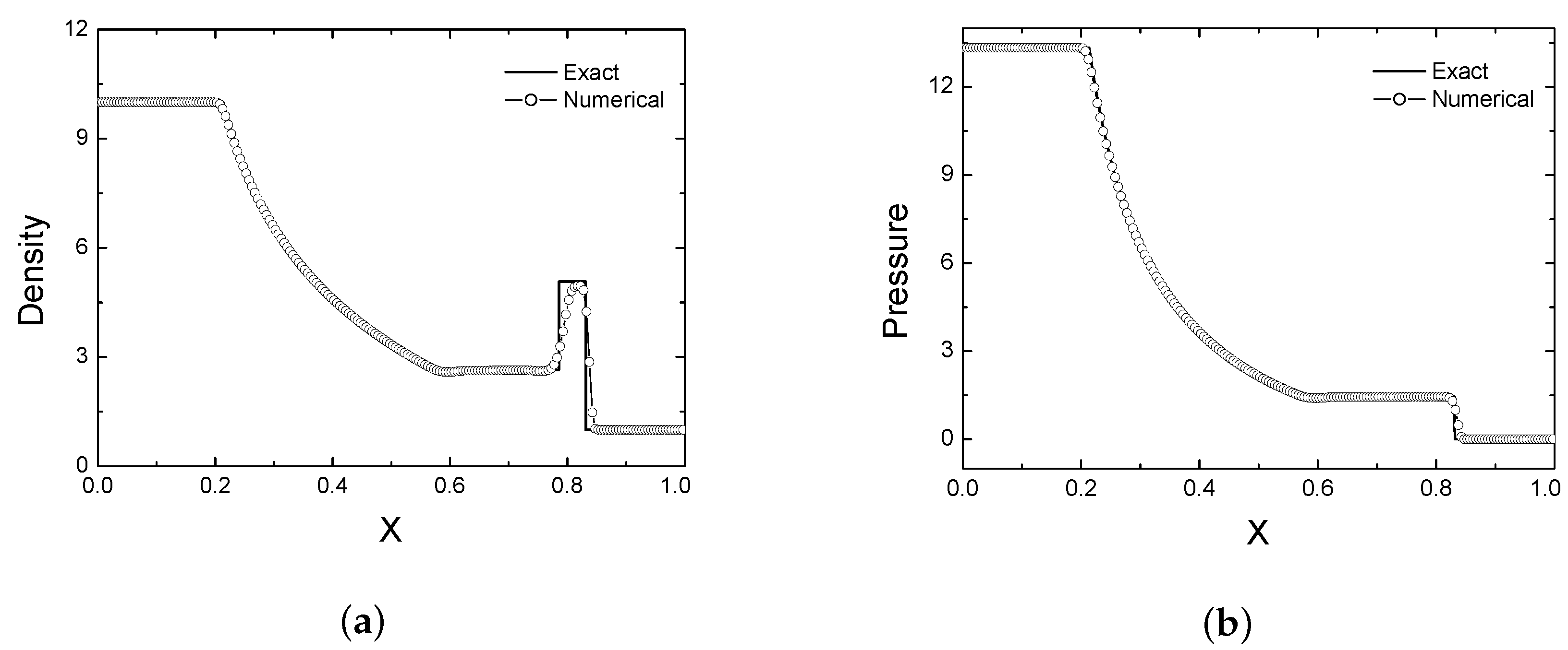
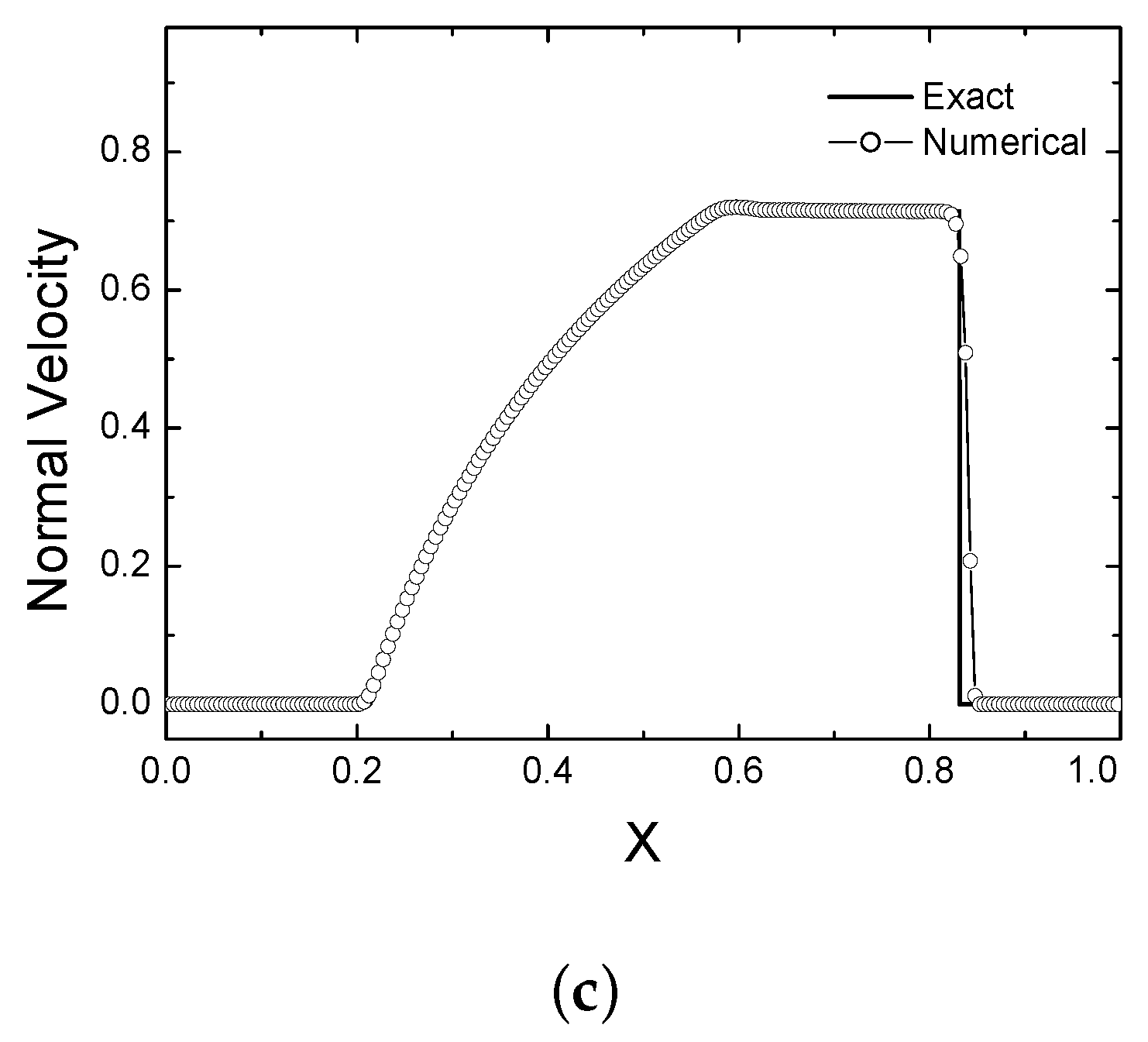
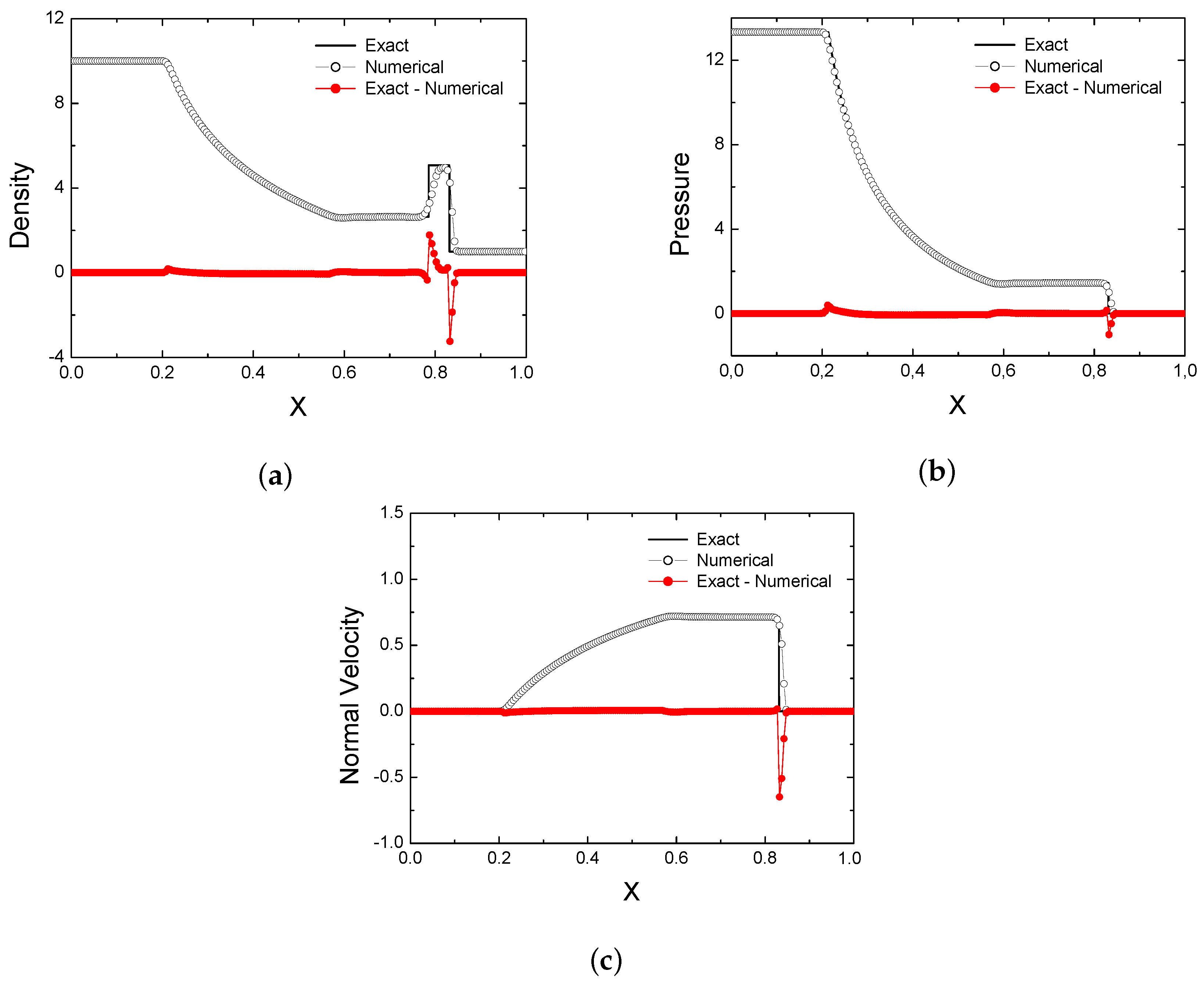
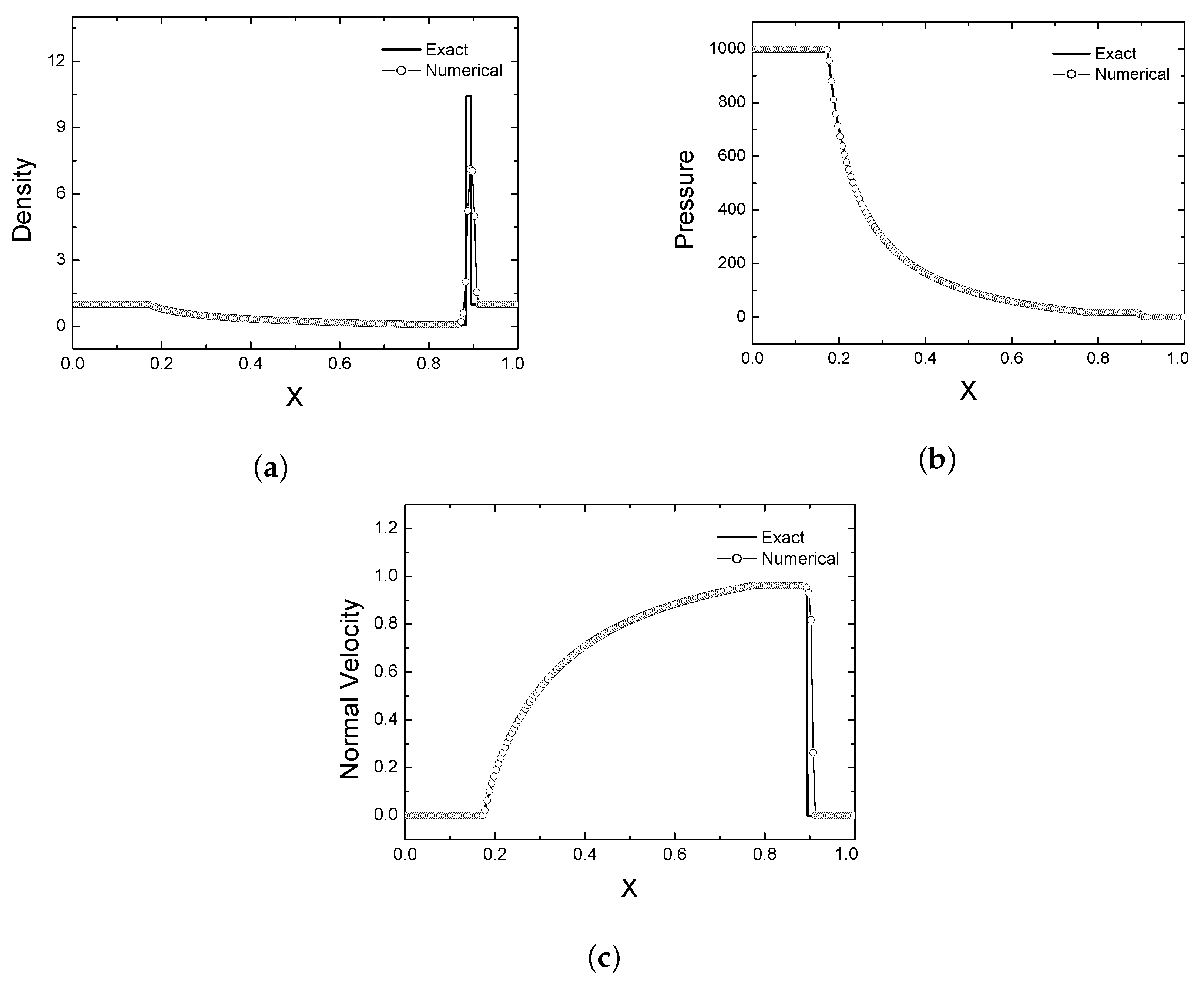
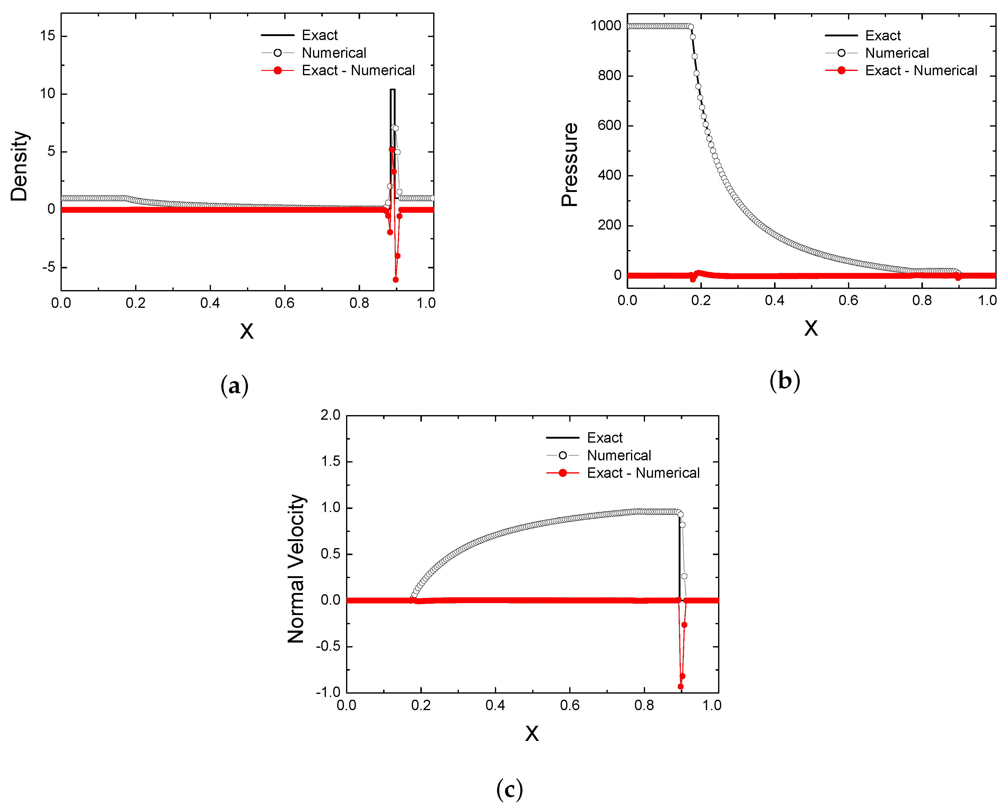
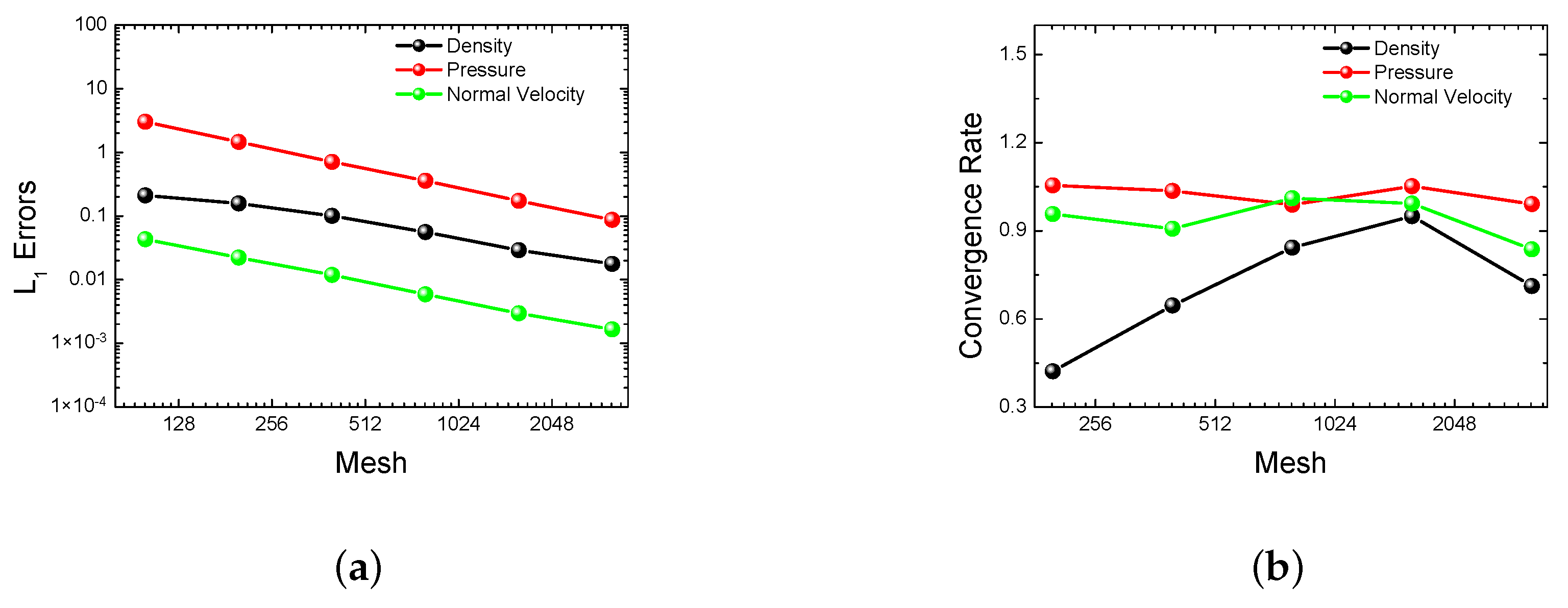
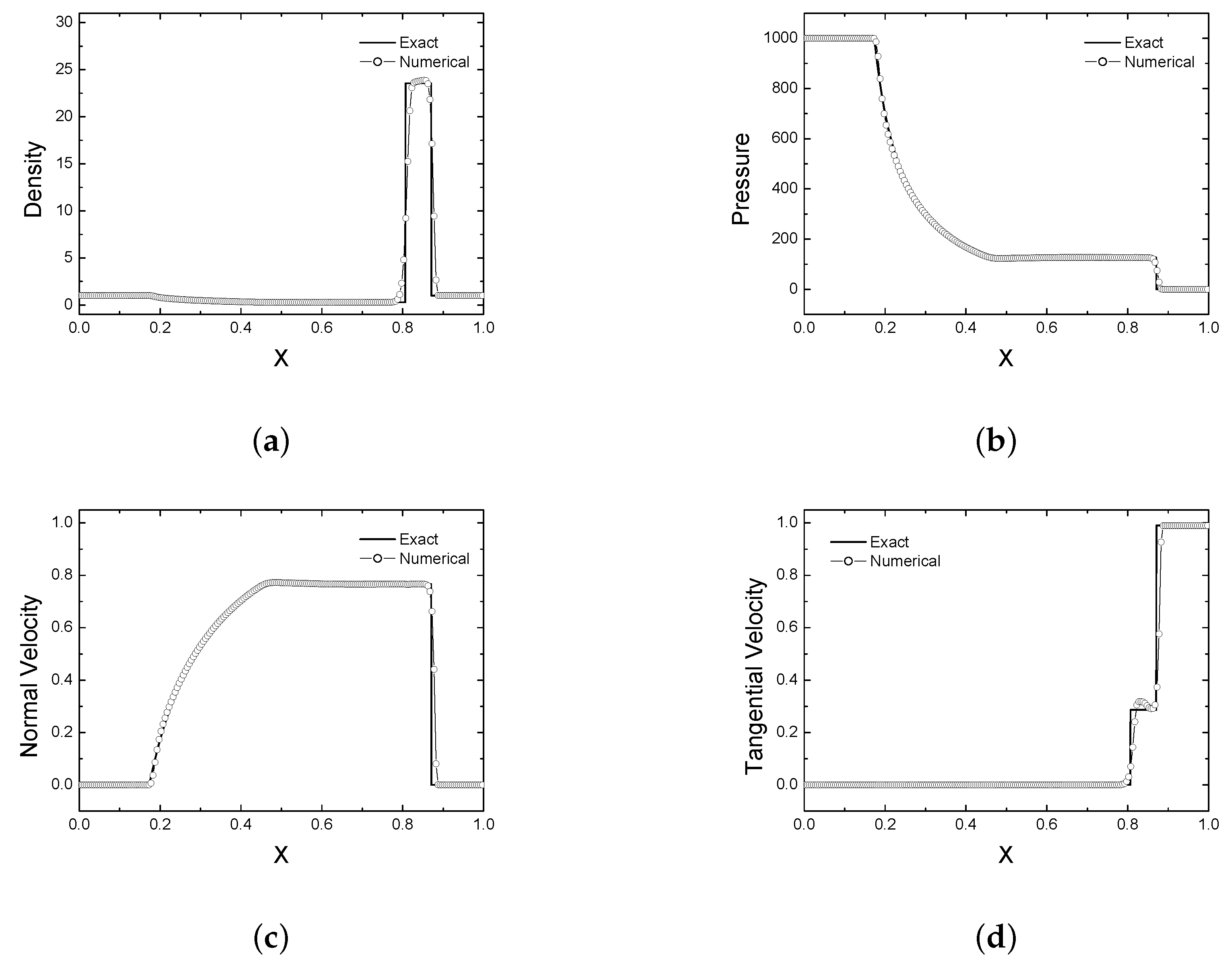
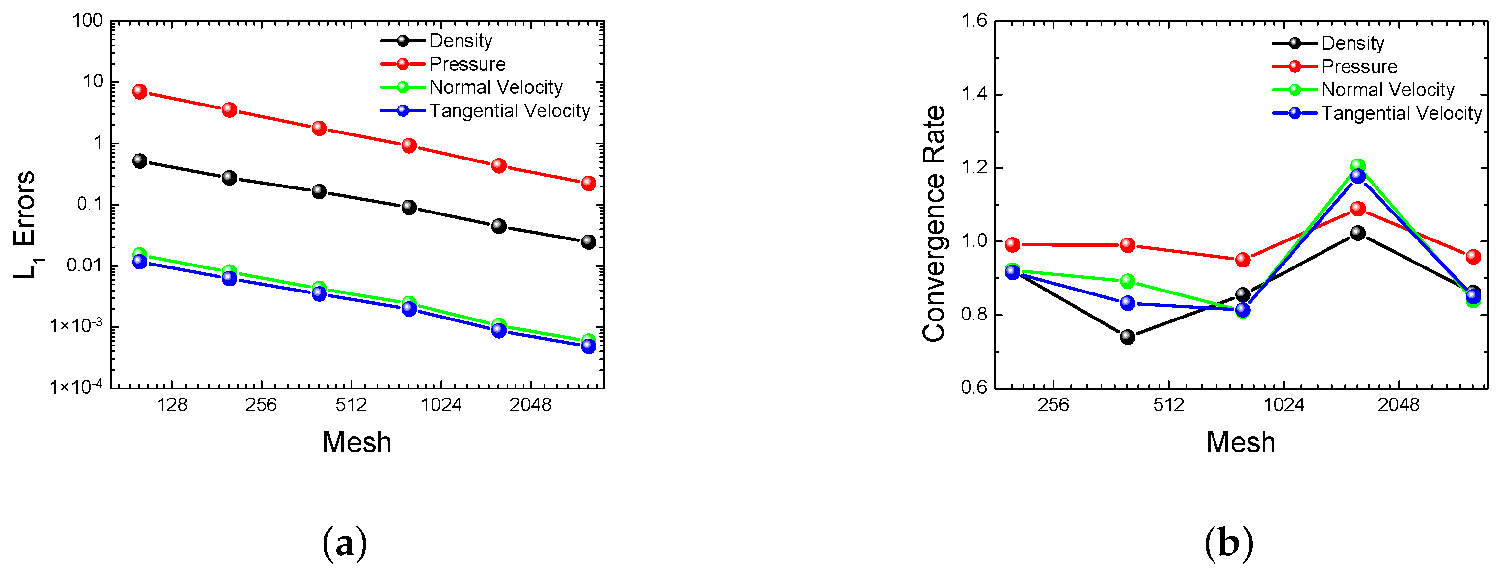
4. Verification
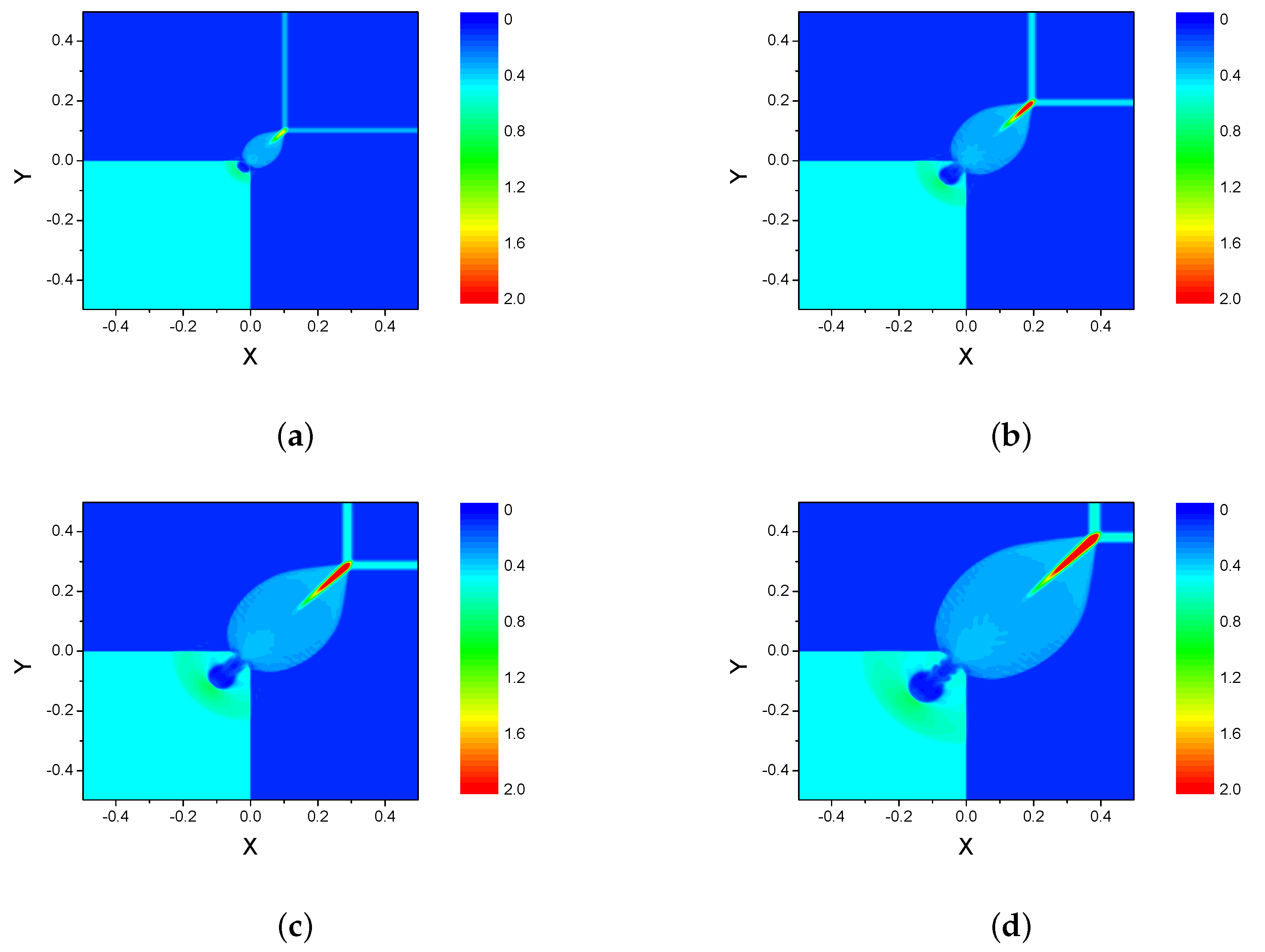
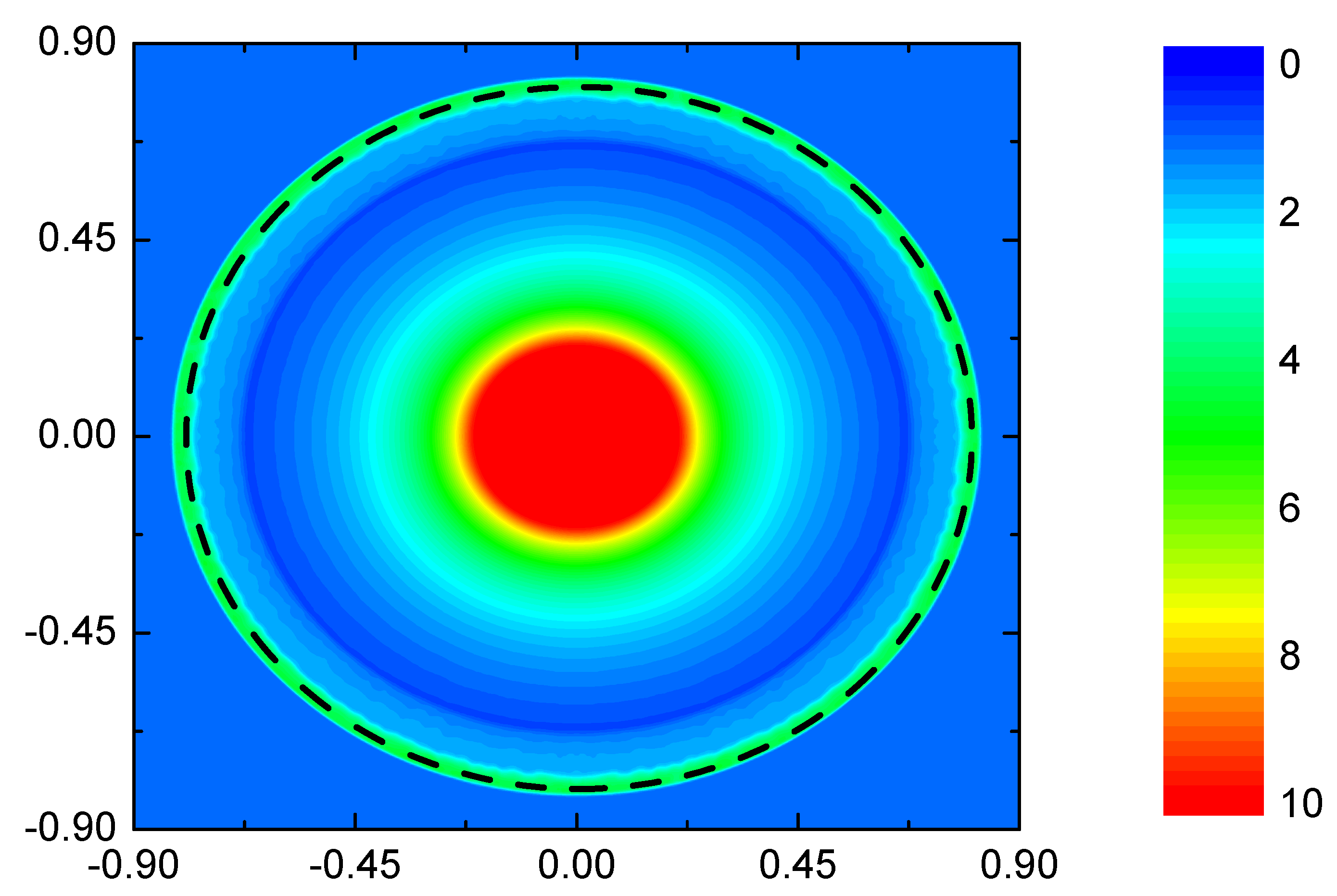
5. Numerical Simulation
6. Discussion and Conclusions
- To increase the order of accuracy on smooth solutions and decrease dissipation at discontinuities, a piecewise parabolic reconstruction is used for the physical variables since they are responsible for the thermodynamic state of the continuous medium [43].
- We use a piecewise-parabolic reconstruction of physical variables although the calculations in the scheme are based on the use of vectors of conservative variables and their flows through cell boundaries. This is due to the fact that they determine the thermodynamic state of a continuous medium. This was emphasized in [43] when studying the accuracy of the discontinuous Galerkin method on the Einfeldt problem.
- When using Rusanov-type methods as part of Godunov’s method, no full spectral problem is solved; this is the case, for instance, when using an equation of state of the Taub–Mathews type [56].
- On the basis of the above computational experiments, we will try to avoid using the MPI technology where possible. The Coarray Fortran technology is a good alternative to develop parallel programs for distributed memory architectures.
- In a number of problems, a significant part of the computational domain is occupied by flows with a high value of the Lorentz factor and low pressure values. In these cases, the energy equation is used in the form:
Author Contributions
Funding
Acknowledgments
Conflicts of Interest
Appendix A
- double precision, allocatable :: array(:)[:]
- irank = this_image()
- isize = num_images()
- Nlocal = N/isize
- i_start_index = (N/isize)*(irank-1)
- if(irank-1 < mod(N,isize)) then
- Nlocal = Nlocal + 1
- i_start_index = i_start_index + irank - 1
- else
- i_start_index = i_start_index + mod(N,isize)
- endif
- allocate(array(Nlocal+4)[*])
- if(irank < isize) then
- array(1)[irank+1] = array(Nlocal+1)array(2)[irank+1] = array(Nlocal+2)
- array(Nlocal+3) = array(3)[irank+1]array(Nlocal+4) = array(4)[irank+1]
- endif
- all
- = (i + i_start_index - 2)*h - h/2.d0
- array(i) = f(x)
- deallocate(array)
- definition of dynamic array located in shared memory between program images;
- definition of variable irank—Coarray Fortran program image number;
- definition of variable isize—the number of images of Coarray Fortran program;
- with known calculation grid size N, calculate the first approximation of the size of the grid Nlocal for the corresponding image of the program;
- calculate the first approximation of the shift index i_start_index of the array part;
- to obtain a uniform distribution of cells over the images, in the first processes the local array size must not exceed the other ones by more than unity;
- add unity to the calculated local size for all first images;
- shift the shift index taking into account the fact that the size of the previous images is greater than the first approximation by unity;
- in the subsequent processes, the first approximation of the grid part size is not recalculated;
- recalculate the shift index with the local sizes of the first images increased by unity;
- this completes the calculation of the shift index and local size;
- allocate memory for array taking into account boundary conditions and/or overlapping areas;
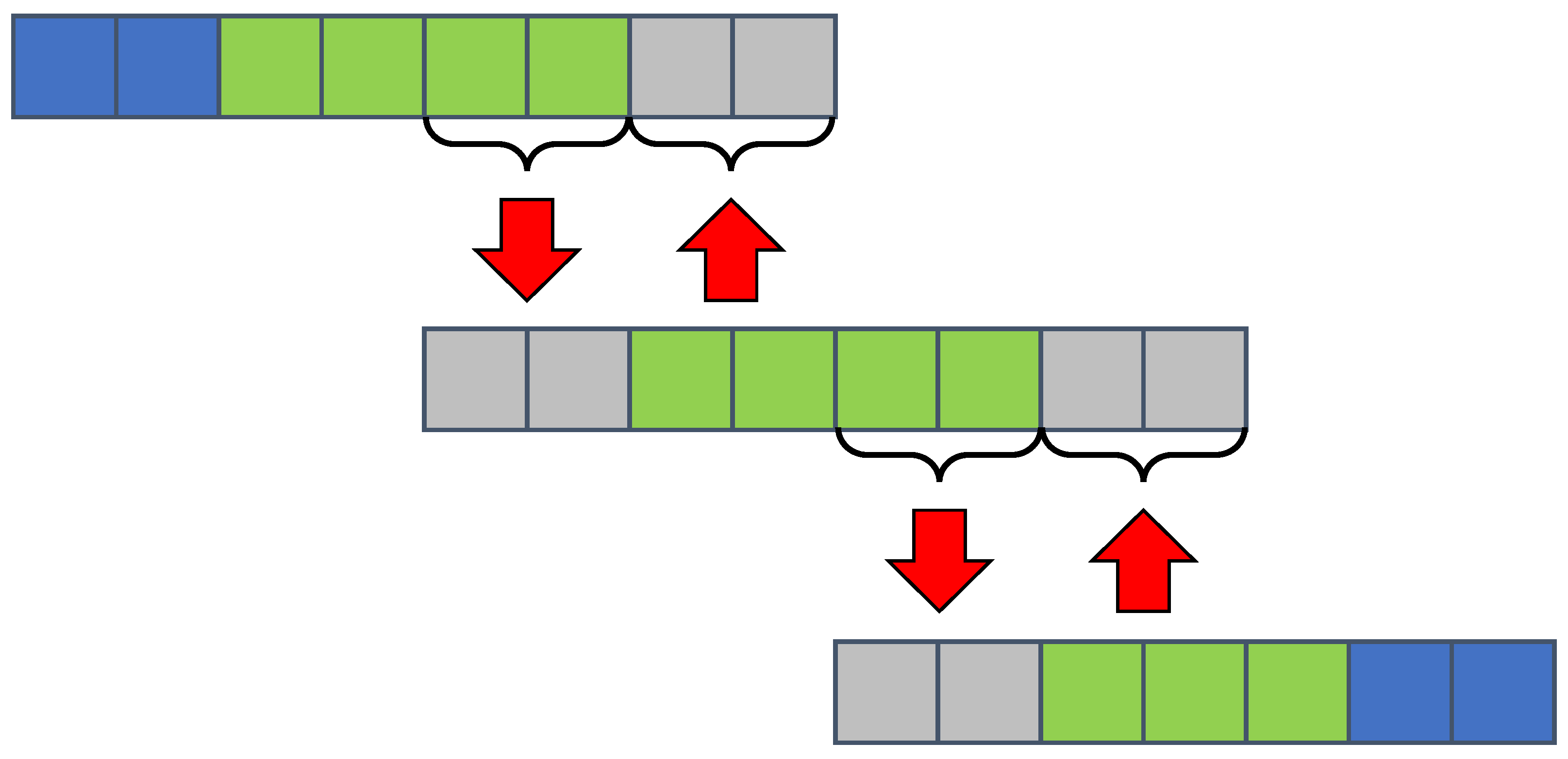
- perform one-way communications with initialization of exchange between the left images of the program;
- write two right extreme values of the local calculation grid into the first two cells—overlapping areas of the next program image;
- write the first two cells of the local calculation grid from the next program image into two rightmost cells—overlapping areas;
- this completes the exchanges between the overlapping areas;
- synchronize data in all images of the Coarray Fortran program;
- calculate the coordinates of the center of cell of size h, taking into account the shift index;
- assign the function value to the corresponding array element;
- remove the memory allocated for the array.
References
- Tyulbashev, S.A.; Chernikov, P.A. Relative variations of the physical parameters of variable extragalactic radio sources. Astron. Rep. 2004, 48, 716–723. [Google Scholar] [CrossRef]
- Chechetkin, V.M.; Dyachenko, V.F.; Ginzburg, S.L.; Paleichik, V.V.; Fimin, N.N.; Sudarikov, A.L. On the generation mechanism of hard cosmic gamma-ray emission from AGN jets. Astron. Rep. 2009, 53, 501–509. [Google Scholar] [CrossRef]
- Chernov, S.V. Polarization Properties of Weakly Relativistic Cylindrical Jets. Astron. Rep. 2019, 63, 910–919. [Google Scholar] [CrossRef]
- Sokolov, V.V.; Bisnovatyi-Kogan, G.S.; Kurt, V.G.; Gnedin, Y.N.; Baryshev, Y.V. Observational constraints on the angular and spectral distributions of photons in gamma-ray burst sources. Astron. Rep. 2006, 50, 612–625. [Google Scholar] [CrossRef] [Green Version]
- Tutukov, A.V.; Cherepashchuk, A.M. Massive close binary stars and gamma-ray bursts. Astron. Rep. 2004, 48, 39–44. [Google Scholar] [CrossRef]
- Chechetkin, V.M.; Dyachenko, V.F.; Ginzburg, S.L.; Fimin, N.N. Dynamics of an ultra-relativistic, collisionless astrophysical plasma. Astron. Rep. 2012, 56, 329–335. [Google Scholar] [CrossRef]
- Tutukov, A.V.; Fedorova, A.V.; Cherepashchuk, A.M. Wolf-Rayet stars with relativistic companions. Astron. Rep. 2013, 57, 657–668. [Google Scholar] [CrossRef]
- Cherepashchuk, A.M. Wolf-Rayet stars and relativistic objects: Distinctions between the mass distributions in close binary systems. Astron. Rep. 2001, 45, 120–137. [Google Scholar] [CrossRef]
- Komissarov, S.S. Simulations of the axisymmetric magnetospheres of neutron stars. Mon. Not. R. Astron. Soc. 2006, 367, 19–31. [Google Scholar] [CrossRef] [Green Version]
- Tutukov, A.V.; Bogomazov, A.I. Radio pulsars in close binaries with neutron stars. Astron. Rep. 2008, 52, 390–402. [Google Scholar] [CrossRef]
- Fateev, V.F.; Davlatov, R.A. Space-Based Gravitational-Wave Detectors: Development of Ground-Breaking Technologies for Future Space-Based Gravitational Gradiometers. Astron. Rep. 2019, 63, 699–709. [Google Scholar] [CrossRef]
- Liu, P.; Zhang, C.-M.; Li, D.; Yang, Y.-Y.; Zhang, J.; Zhang, J.-W. The Simulation of Orbit Decay of Double Neutron Star System PSR J1906+0746 by the Gravitational Wave Radiation. Astron. Rep. 2019, 63, 1090–1094. [Google Scholar] [CrossRef]
- Glushak, A.P. Microquasar jets in the supernova remnant G11.2-0.3. Astron. Rep. 2014, 58, 6–15. [Google Scholar] [CrossRef]
- Barkov, M.V.; Bisnovatyi-Kogan, G.S. Interaction of a cosmological gamma-ray burst with a dense molecular cloud and the formation of jets. Astron. Rep. 2005, 49, 24–35. [Google Scholar] [CrossRef]
- Istomin, Y.N.; Komberg, B.V. Gamma-ray bursts as a result of the interaction of a shock from a supernova and a neutron-star companion. Astron. Rep. 2002, 46, 908–917. [Google Scholar] [CrossRef]
- Artyukh, V.S. Phenomenological model for the evolution of radio galaxies such as Cygnus A. Astron. Rep. 2015, 59, 520–524. [Google Scholar] [CrossRef]
- Artyukh, V.S. Effect of Aberration on the Estimated Parameters of Relativistic Radio Jets. Astron. Rep. 2018, 62, 436–439. [Google Scholar] [CrossRef]
- Butuzova, M.S. Search for differences in the velocities and directions of the kiloparsec-scale jets of quasars with and without X-ray emission. Astron. Rep. 2016, 60, 313–321. [Google Scholar] [CrossRef]
- Butuzova, M.S. The Blazar OJ 287 Jet from Parsec to Kiloparsec Scales. Astron. Rep. 2021, 65, 635–644. [Google Scholar] [CrossRef]
- Malov, I.F.; Machabeli, G.Z.; Malofeev, V.M. A new model of a magnetar. Astron. Rep. 2003, 47, 232–239. [Google Scholar] [CrossRef]
- Belyaev, V.S.; Bisnovatyi-Kogan, G.S.; Gromov, A.I.; Zagreev, B.V.; Lobanov, A.V.; Matafonov, A.P.; Moiseenko, S.G.; Toropina, O.D. Numerical Simulations of Magnetized Astrophysical Jets and Comparison with Laboratory Laser Experiments. Astron. Rep. 2018, 62, 162–182. [Google Scholar] [CrossRef] [Green Version]
- Krauz, V.I.; Mitrofanov, K.N.; Kharrasov, A.M.; Ilyichev, I.V.; Myalton, V.V.; Ananyev, S.S.; Beskin, V.S. Laboratory Modeling of the Rotation of Jets Ejected from Young Stellar Objects at Studies the Azimuthal Structure of an Axial Jet at the PF-3 Facility. Astron. Rep. 2021, 65, 26–44. [Google Scholar] [CrossRef]
- Kulikov, I. A new code for the numerical simulation of relativistic flows on supercomputers by means of a low-dissipation scheme. Comput. Phys. Commun. 2020, 257, 107532. [Google Scholar] [CrossRef]
- Godunov, S.K. A difference method for numerical calculation of discontinuous solutions of the equations of hydrodynamics. Mat. Sb. 1959, 47, 271–306. [Google Scholar]
- Godunov, S.K.; Manuzina, Y.D.; Nazar’eva, M.A. Experimental analysis of convergence of the numerical solution to a generalized solution in fluid dynamics. Comput. Math. Math. Phys. 2011, 51, 88–95. [Google Scholar] [CrossRef]
- Godunov, S.K.; Kulikov, I.M. Computation of Discontinuous Solutions of Fluid Dynamics Equations with Entropy Nondecrease Guarantee. Comput. Math. Math. Phys. 2014, 54, 1012–1024. [Google Scholar] [CrossRef]
- Godunov, S.K.; Denisenko, V.V.; Klyuchinskii, D.V.; Fortova, S.V.; Shepelev, V.V. Study of Entropy Properties of a Linearized Version of Godunov’s Method. Comput. Math. Math. Phys. 2020, 60, 628–640. [Google Scholar] [CrossRef]
- Godunov, S.K.; Klyuchinskii, D.V.; Fortova, S.V.; Shepelev, V.V. Experimental Studies of Difference Gas Dynamics Models with Shock Waves. Comput. Math. Math. Phys. 2018, 58, 1201–1216. [Google Scholar] [CrossRef]
- Kulikov, I.M. A Low-Dissipation Numerical Scheme Based on a Piecewise Parabolic Method on a Local Stencil for Mathematical Modeling of Relativistic Hydrodynamic Flows. Numer. Anal. Appl. 2020, 13, 117–126. [Google Scholar] [CrossRef]
- Godunov, S.K. Thermodynamic formalization of the fluid dynamics equations for a charged dielectric in an electromagnetic field. Comput. Math. Math. Phys. 2012, 52, 787–799. [Google Scholar] [CrossRef]
- Godunov, S.K. About inclusion of Maxwell’s equations in systems relativistic of the invariant equations. Comput. Math. Math. Phys. 2013, 53, 1179–1182. [Google Scholar] [CrossRef]
- Rusanov, V.V. The calculation of the interaction of non-stationary shock waves with barriers. Comput. Math. Math. Phys. 1961, 1, 267–279. [Google Scholar]
- Kolgan, V.P. Application of the principle of minimizing the derivative to the construction of finite-difference schemes for computing discontinuous gas flows. Uch. Zap. Tsentr. Aerogidrodin. Inst. 1972, 3, 68–77. [Google Scholar]
- Kurganov, A.; Tadmor, E. New High-Resolution Central Schemes for Nonlinear Conservation Laws and Convection-Diffusion Equation. J. Comput. Phys. 2000, 160, 214–282. [Google Scholar] [CrossRef] [Green Version]
- Popov, M.; Ustyugov, S. Piecewise parabolic method on local stencil for gasdynamic simulations. Comput. Math. Math. Phys. 2007, 47, 1970–1989. [Google Scholar] [CrossRef]
- Popov, M.; Ustyugov, S. Piecewise parabolic method on a local stencil for ideal magnetohydrodynamics. Comput. Math. Math. Phys. 2008, 48, 477–499. [Google Scholar] [CrossRef]
- Titarev, V.A.; Toro, E.F. ADER schemes for three-dimensional nonlinear hyperbolic systems. J. Comput. Phys. 2005, 204, 715–736. [Google Scholar] [CrossRef]
- Kulikov, I.M.; Chernykh, I.G.; Glinskiy, B.M.; Protasov, V.A. An Efficient Optimization of Hll Method for the Second Generation of Intel Xeon Phi Processor. Lobachevskii J. Math. 2018, 39, 543–551. [Google Scholar] [CrossRef]
- Kulikov, I.; Vorobyov, E. Using the PPML approach for constructing a low-dissipation, operator-splitting scheme for numerical simulations of hydrodynamic flows. J. Comput. Phys. 2016, 317, 318–346. [Google Scholar] [CrossRef] [Green Version]
- Kulikov, I.M.; Chernykh, I.G.; Tutukov, A.V. A New Parallel Intel Xeon Phi Hydrodynamics Code for Massively Parallel Supercomputers. Lobachevskii J. Math. 2018, 39, 1207–1216. [Google Scholar] [CrossRef]
- Kulikov, I.; Chernykh, I.; Tutukov, A. A New Hydrodynamic Code with Explicit Vectorization Instructions Optimizations that Is Dedicated to the Numerical Simulation of Astrophysical Gas Flow. I. Numerical Method, Tests, and Model Problems. Astrophys. J. Suppl. Ser. 2019, 243, 4. [Google Scholar] [CrossRef]
- Kulikov, I. Using a Combination of Godunov and Rusanov Solvers based on the Piecewise Parabolic Reconstruction of Primitive Variables for Numerical Simulation of Supernovae Ia Type Explosion. Lobachevskii J. Math. 2022; in print. [Google Scholar]
- Kriksin, Y.A.; Tishkin, V.F. Variational Entropic Regularization of the Discontinuous Galerkin Method for Gasdynamic Equations. Math. Model. Comput. Simulations 2019, 11, 1032–1040. [Google Scholar] [CrossRef]
- Tunik, Y.V. Numerical Solution of Test Problems Using a Modified Godunov Scheme. Comput. Math. Math. Phys. 2018, 58, 1573–1584. [Google Scholar] [CrossRef]
- Kulikov, I.M.; Chernykh, I.G.; Sapetina, A.F.; Lomakin, S.V.; Tutukov, A.V. A New Rusanov-Type Solver with a Local Linear Solution Reconstruction for Numerical Modeling of White Dwarf Mergers by Means Massive Parallel Supercomputers. Lobachevskii J. Math. 2020, 41, 1485–1491. [Google Scholar] [CrossRef]
- Kulikov, I.M. On a Modification of the Rusanov Solver for the Equations of Special Relativistic Magnetic Hydrodynamics. J. Appl. Ind. Math. 2020, 14, 524–531. [Google Scholar] [CrossRef]
- Barkov, M.; Bosch-Ramon, V. Relativistic hydrodynamical simulations of the effects of the stellar wind and the orbit on high-mass microquasar jets Get access Arrow. Mon. Not. R. Astron. Soc. 2022, 510, 3479–3494. [Google Scholar] [CrossRef]
- Reshetova, G.; Cheverda, V.; Khachkova, T. A Comparison of MPI/OpenMP and Coarray Fortran for Digital Rock Physics Application. Lect. Notes Comput. Sci. 2019, 11657, 232–244. [Google Scholar]
- Reshetova, G.; Cheverda, V.; Khachkova, T. Numerical Experiments with Digital Twins of Core Samples for Estimating Effective Elastic Parameters. Commun. Comput. Inf. Sci. 2019, 1129, 290–301. [Google Scholar]
- Reshetova, G.; Cheverda, V.; Koinov, V. Comparative Efficiency Analysis of MPI Blocking and Non-blocking Communications with Coarray Fortran. Commun. Comput. Inf. Sci. 2022, 1510, 322–336. [Google Scholar]
- Wang, Y.; Li, Z. GridFOR: A Domain Specific Language for Parallel Grid-Based Applications. Int. J. Parallel Program. 2016, 44, 427–448. [Google Scholar] [CrossRef]
- Kataev, N.; Kolganov, A. The experience of using DVM and SAPFOR systems in semi automatic parallelization of an application for 3D modeling in geophysics. J. Supercomput. 2019, 75, 7833–7843. [Google Scholar] [CrossRef]
- Shterenlikht, A.; Cebamanos, L. MPI vs. Fortran coarrays beyond 100k cores: 3D cellular automata. Parallel Comput. 2019, 84, 37–49. [Google Scholar] [CrossRef]
- Guo, P.; Wu, J. One-Sided Communication in Coarray Fortran: Performance Tests on TH-1A. Lect. Notes Comput. Sci. 2018, 11337, 21–33. [Google Scholar]
- Landau, L.D.; Lifshitz, E.M. The Classical Theory of Fields, 4th ed.; Elsevier: Amsterdam, The Netherlands, 1987; p. 402. [Google Scholar]
- Mathews, W. The Hydromagnetic Free Expansion of a Relativistic Gas. Astrophys. J. 1971, 165, 147–164. [Google Scholar] [CrossRef]
- Perucho, M.; Marti, J.M. A numerical simulation of the evolution and fate of a Fanaroff-Riley type I jet. The case of 3C 31. Mon. Not. R. Astron. Soc. 2007, 382, 526–542. [Google Scholar] [CrossRef] [Green Version]
- Perucho, M.; Marti, J.M.; Quilis, V. Long-term FRII jet evolution in dense environments. Mon. Not. R. Astron. Soc. 2022, 510, 2084–2096. [Google Scholar] [CrossRef]


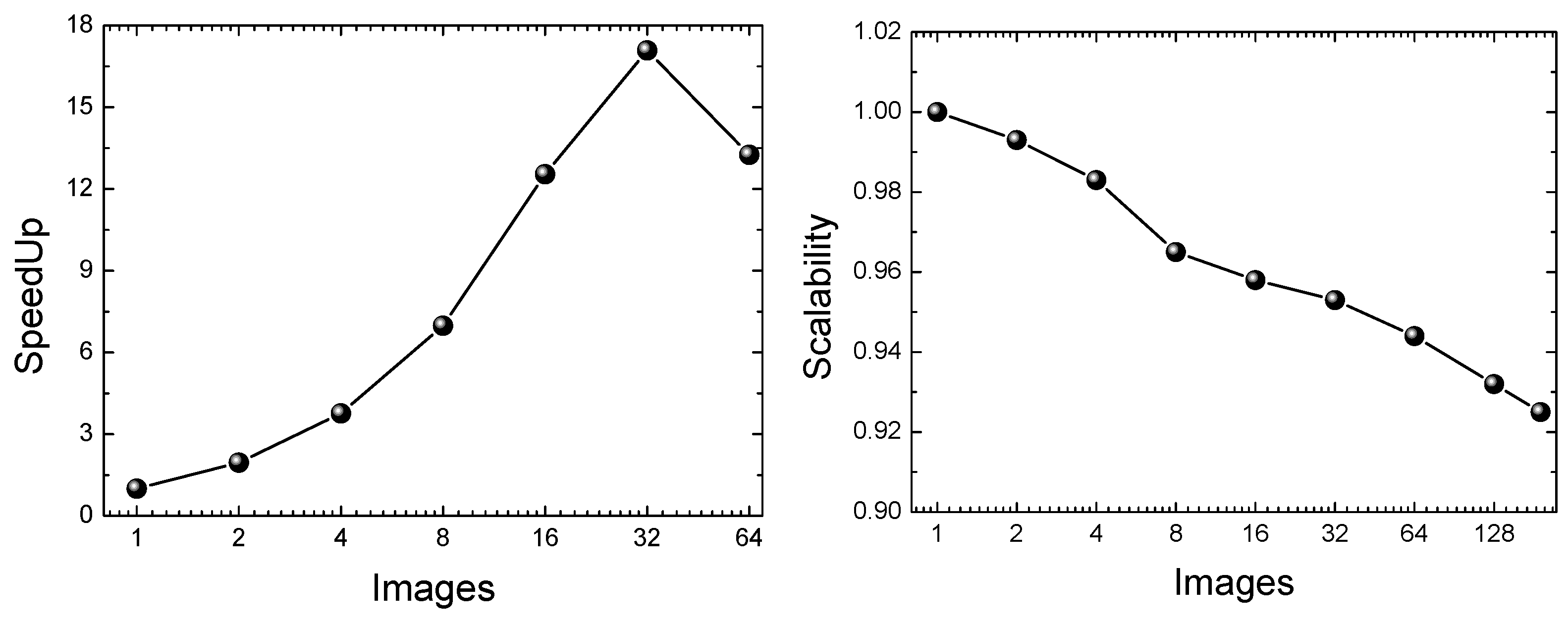
| Nodes | Sockets | Cores | Threads | Images | Time (s) |
|---|---|---|---|---|---|
| 1 | 1 | 1 | 1 | 1 | 27.542 |
| 1 | 1 | 2 | 1 | 2 | 14.724 |
| 1 | 1 | 1 | 2 | 2 | 14.443 |
| 1 | 2 | 1 | 1 | 2 | 14.122 |
| 2 | 1 | 1 | 1 | 2 | 14.072 |
| 1 | 1 | 2 | 2 | 4 | 7.345 |
| 1 | 1 | 4 | 1 | 4 | 7.485 |
| 1 | 2 | 1 | 2 | 4 | 7.395 |
| 2 | 1 | 2 | 1 | 4 | 7.398 |
| 2 | 1 | 1 | 2 | 4 | 7.318 |
| 2 | 2 | 1 | 1 | 4 | 7.378 |
| 1 | 1 | 8 | 1 | 8 | 3.952 |
| 1 | 1 | 4 | 2 | 8 | 4.045 |
| 1 | 2 | 2 | 2 | 8 | 4.051 |
| 1 | 2 | 4 | 1 | 8 | 3.985 |
| 2 | 2 | 1 | 2 | 8 | 3.945 |
| 2 | 1 | 2 | 2 | 8 | 3.946 |
| 2 | 2 | 2 | 1 | 8 | 3.971 |
Publisher’s Note: MDPI stays neutral with regard to jurisdictional claims in published maps and institutional affiliations. |
© 2022 by the authors. Licensee MDPI, Basel, Switzerland. This article is an open access article distributed under the terms and conditions of the Creative Commons Attribution (CC BY) license (https://creativecommons.org/licenses/by/4.0/).
Share and Cite
Kulikov, I.; Chernykh, I.; Karavaev, D.; Prigarin, V.; Sapetina, A.; Ulyanichev, I.; Zavyalov, O. A New Parallel Code Based on a Simple Piecewise Parabolic Method for Numerical Modeling of Colliding Flows in Relativistic Hydrodynamics. Mathematics 2022, 10, 1865. https://doi.org/10.3390/math10111865
Kulikov I, Chernykh I, Karavaev D, Prigarin V, Sapetina A, Ulyanichev I, Zavyalov O. A New Parallel Code Based on a Simple Piecewise Parabolic Method for Numerical Modeling of Colliding Flows in Relativistic Hydrodynamics. Mathematics. 2022; 10(11):1865. https://doi.org/10.3390/math10111865
Chicago/Turabian StyleKulikov, Igor, Igor Chernykh, Dmitry Karavaev, Vladimir Prigarin, Anna Sapetina, Ivan Ulyanichev, and Oleg Zavyalov. 2022. "A New Parallel Code Based on a Simple Piecewise Parabolic Method for Numerical Modeling of Colliding Flows in Relativistic Hydrodynamics" Mathematics 10, no. 11: 1865. https://doi.org/10.3390/math10111865