Damping Optimization of Linear Vibrational Systems with a Singular Mass Matrix

Abstract

We present two novel results for small damped oscillations described by the vector differential equation $M\ddot{x}+C\dot{x}+Kx=0$, where the mass matrix M can be singular, but standard deflation techniques cannot be applied. The first result is a novel formula for the solution X of the Lyapunov equation $A^{T}X+XA=-I$, where $A=A\left(v\right)$ is obtained from $M,C\left(v\right)\in {\mathbb{R}}^{n\times n}$, and $K\in {\mathbb{R}}^{n\times n}$, which are the so-called mass, damping, and stiffness matrices, respectively, and $\mathrm{rank}\left(M\right)=n-1$. Here, $C\left(v\right)$ is positive semidefinite with $\mathrm{rank}\left(C\right(v\left)\right)=1$. Using the obtained formula, we propose a very efficient way to compute the optimal damping matrix. The second result was obtained for a different structure, where we assume that $dim\left(\mathcal{N}\right(M\left)\right)\ge 1$ and internal damping exists (usually a small percentage of the critical damping). For this structure, we introduce a novel linearization, i.e., a novel construction of the matrix A in the Lyapunov equation $A^{T}X+XA=-I$, and a novel optimization process. The proposed optimization process computes the optimal damping $C\left(v\right)$ that minimizes a function $v\mapsto \mathrm{trace}\left(ZX\right)$ (where Z is a chosen symmetric positive semidefinite matrix) using the approximation function $g\left(v\right)=c_v+\frac{a}{v}+bv$, for the trace function $f\left(v\right)\doteq \mathrm{trace}\left(ZX\right(v\left)\right)$. Both results are illustrated with several corresponding numerical examples.

1. Introduction

We consider small damped oscillations in the absence of gyroscopic forces, described by the vector differential equation

$$\begin{array}{c}\hfill M\ddot{x}+C\dot{x}+Kx=0,\\ \hfill x\left(0\right)=x_0,\dot{x}\left(0\right)={\dot{x}}_0,\end{array}$$

(1)

where $M,C,$ and K (mass, damping, and stiffness matrices, respectively) are real, symmetric matrices of order n.

The main problem considered in this paper is the derivation (or computation) of the optimal damping for vibrating systems, such as those mentioned above, for the case where the damping matrix becomes singular. The problem of damping optimization is part of a very interesting and active research area where several different approaches exist. Damping optimization is usually a very demanding problem; moreover, the problem of optimizing damping positions with viscosities still has no satisfactory solution.

Damping optimization contains two different sub-problems, including one in which the mass matrix is non-singular and one in which the mass matrix can be singular.

Damping optimization with non-singular mass has been widely investigated during the last two decades. Some of the results concerning the so-called stationary system can be found in [1,2,3,4,5,6,7,8,9]. A more detailed description of these references can be found in [10].

On the other hand, the problem of non-stationary systems has been considered in [10,11,12].

Here, M, K, and C are large, usually of order $n>\mathcal{O}\left(1000\right)$, and do not have a prescribed structure; M and K are very often diagonal, tridiagonal, or some other structure, depending on the application. It is important to emphasize that the assumptions concerning the mass and the damping matrix do not allow the use of standard deflation techniques as in [13,14], nor the frequency domain approach from [15] because M and C cannot be diagonalized simultaneously.

A damping matrix can be defined in several different ways. One of the most common ways is that $C=C_{in}+C_{ext}\left(v\right)$, where $C_{in}$ represents internal damping, and only the external damping part depends on the parameters $v>0$ (called viscosities). Moreover, external damping can be written as $C_{ext}\left(v\right)=v{C}_i$, where $C_i$ determines the geometry of the i-th damper, and it has a small rank, so that $C_{ext}\left(v\right)$ is a semidefinite matrix.

Internal damping, $C_{in}$, can be modeled in different ways. The most popular is the classical Rayleigh damping:

$$C_{in}=\alpha M+\beta K.$$

However, throughout this paper, we use the definition that internal damping is a small multiple of critical damping; that is, in the case of critical damping

$$C_{in}=\alpha M^{1/2}\sqrt{M^{-1/2}K{M}^{-1/2}}{M}^{1/2},$$

(2)

see, e.g., [16,17]. More details regarding the model can be found in [6,7,11,16,18,19,20,21,22].

There are several different (damping) optimization criteria, and the most common ones are based on the asymptotic approach or the approach in which the damping criterion is based on an infinite time scale. For example, in [12,23,24,25,26], the optimal displacement or optimal damper positions are based on the criterion that considers asymptotical behavior. On the other hand, in [10], the optimization criteria are defined over the basic period of the periodic external force $g\left(t\right)$.

In this paper, we consider the optimization process based on the so-called energy minimization criterion, which is equivalent to the minimization of the trace of the solution of the Lyapunov equation

$$A^{T}X+XA=-I.$$

(3)

For the case where M can be singular, the matrix A that depends on M, D, and K must be carefully constructed because standard linearization is not possible. The particular construction of the matrix A is one of our novel results.

Further, the optimal damping is obtained from the following optimization process:

$$v={\mathrm{argmin}}_{v}f\left(v\right)\doteq {\mathrm{argmin}}_v\mathrm{trace}\left(ZX\left(v\right)\right),$$

(4)

where the damping matrix is given as $D\left(v\right)=C_{in}+v{C}_{ex}$. For the physical background of this penalty function, see [19,20,27].

Here, Z is a symmetric positive semidefinite matrix, usually defined as

$$Z=Z_1\oplus Z_1,\mathrm{where}{Z}_1\in {\mathbb{R}}^{n\times n},\mathrm{and}{Z}_1=\left[\begin{array}{ccc}0& 0& 0\\ 0& I_s& 0\\ 0& 0& 0\end{array}\right],$$

(5)

where $I_s$ denotes an identity matrix of dimension s.

As was shown in [3] (or [27]), the above optimization criterion is equivalent to the minimization of the mean value of the total energy of all initial data. More details about the construction of the matrix Z can be found in [3].

In this paper, we consider two different cases (two different structures) of damping matrices. In the first part of the paper, we assume that the damping matrix is given as $D\left(v\right)=v{C}_{ex}$, that is, that the internal damping is zero ($C_{in}=0$). For this particular case, we additionally assume that the dimension of the null space of the mass matrix $dim\left(\mathcal{N}\right(M\left)\right)=1$. For this case, we derive the formula for the solution X of the Lyapunov Equation (3) as a function of v; this allows us to discuss some properties of the solution and to find the graph of the meromorphic function $v\mapsto \mathrm{trace}\left(ZX\right)$ by finding its poles and performing a corresponding partial fraction decomposition.

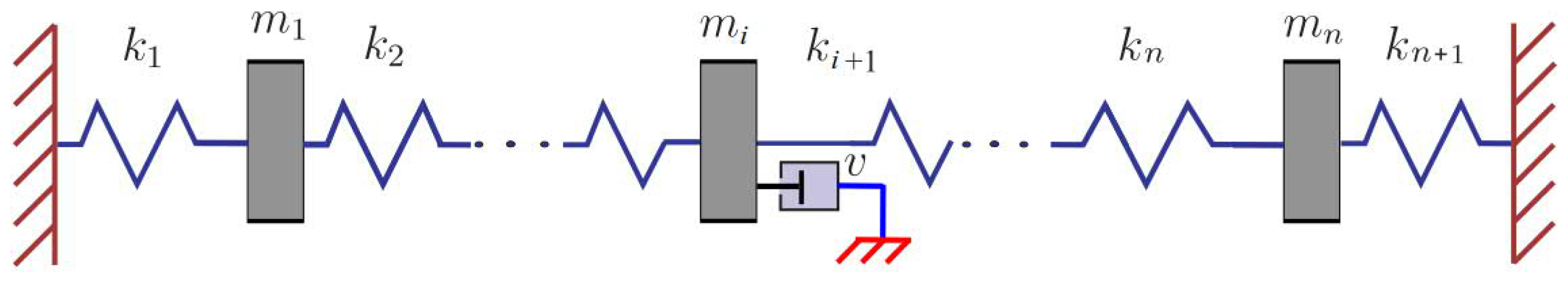
An example of such a system is the so-called n-mass oscillator or oscillator ladder (Figure 1), where

$$M=\mathrm{diag}(m_1,m_2,\dots ,m_n),$$

(6)

$$K=\left[\begin{array}{ccccc}{k}_1+k_2& -k_2& & & \\ -k_2& k_2+k_3& -k_3& & \\ & \ddots & \ddots & \ddots & \\ & & -k_{n-1}& k_{n-1}+k_n& -k_n\\ & & & -k_n& k_n+k_{n+1}\end{array}\right],$$

(7)

$$D\equiv C_{in}+C\left(v\right)=C_{in}+v{e}_i{e}_i^T.$$

(8)

Here, $m_i\ge 0$ are the masses, $k_i>0$ are the spring constants or stiffnesses, $e_i$ is the i-th canonical basis vector, and v is the viscosity of the damper applied on the i-th mass. Note that, for the system presented in Figure 1, the rank of the matrix $C\left(v\right)$ is one.

The first part of this paper is devoted to structures similar to the one in Figure 1. For example, in the mass-spring system shown in (6)–(8), if one of the masses, for example, $m_n$, were to vanish (that is, if one mass were substituted with a damper or if it were sufficiently smaller then the others such that it could be neglected), then the mass matrix M would be singular, and the standard linearization would not be possible. In fact, in such a case, we could not prescribe the initial velocity ${\dot{x}}_n\left(0\right)$, and the phase space would have a dimension less than $2n$. This would be even more the case if there were no damping at the position in question; then, we could not even prescribe $x_n\left(0\right)$. More details on this type of structure can be found in [11].

Since we have a strong structure in the first part of the paper ($C_{in}=0$ and $dim\left(\mathcal{N}\right(M\left)\right)=1$) and, as a result, we present a formula for the solution $X\left(v\right)$, we refer to this as the“theoretical part”. As we see in the numerical examples, the structures are extremely unstable without internal damping, and it is hard to calculate any quantities for $dim\left(\mathcal{N}\right(M\left)\right)\ge 1$ when $C_{in}=0$.

Thus, in the second part of the paper, we assume that $dim\left(\mathcal{N}\right(M\left)\right)\ge 1$ and $C_{in}>0$ (usually a small percentage of the critical damping). The second part of the paper is the “numerical part” or “numerical point of view”. In this part, we present a novel construction of the matrix A in the Lyapunov Equation (3) and a novel optimization process that is based on the properties of the formula obtained in the first part of the paper and the new approximated (projected) Lyapunov equation. Our optimization process is based on the idea of approximating the trace function $f\left(v\right)\doteq \mathrm{trace}\left(ZX\right(v\left)\right)$ with its approximation

$$g\left(v\right)=c_v+\frac{a}{v}+bv,a,b>0,$$

(9)

which allows us to find the minima. Here, a, b, and $c_v$ are obtained by simple interpolation using the approximate trace function $\tilde{f}\left(v\right)\doteq \mathrm{trace}\left(Z\tilde{X}\left(v\right)\right)$ through the three points $v_1,v_2,$ and $v_3$, where $\tilde{X}$ is the solution of the approximate Lyapunov equation

$${\tilde{A}}^T\tilde{X}+\tilde{X}\tilde{A}=-I,$$

(10)

and $\tilde{A}$ is the projected matrix A of smaller dimension.

A similar formula was obtained in [20] for the case $\mathrm{rank}\left(D\right(v\left)\right)=1$, while the case $\mathrm{rank}\left(D\right(v\left)\right)>1$ seems to be more difficult to handle, as shown in [10,21].

As we see in the section that includes the numerical illustrations, our approach speeds up the viscosity optimization process by 3 to 10 times.

We would like to emphasize that damping optimization using criterion (4) requires solving the Lyapunov Equation (3) numerous times, which may be inefficient, as well as memory- and time-consuming. However, most of the usual (engineering) approaches that assume that all three matrices M, C, and K can be simultaneously diagonalized are inappropriate here due to the structure of the damping matrix.

The paper is organized as follows. In Section 2, we present the novel formula for the solution X of the Lyapunov Equation (3) as the function of the viscosity parameter v. In Section 3, we present a novel approach to calculating the optimal damping matrix D, which includes quasi-optimal positions together with the corresponding optimal viscosity parameter. At the end of Section 3, we illustrate the main results using a numerical example.

2. The Singular Mass Case, $dim\left(\mathcal{N}\right(\mathbf{M}\left)\right)=\mathbf{1}$

As we emphasized in the introduction, the damped mass-spring system with a singular mass matrix deserves special treatment since standard linearization is not possible. For this purpose, we use the results from the book [11] by Krešimir Veselić on the linearization of damped mass-spring systems with singular mass.

Without losing on generality, we assume that $\mathsf{\Phi }$ is a real non-singular matrix such that

$$\begin{array}{c}\hfill {\mathsf{\Phi }}^{T}M\mathsf{\Phi }=\left[\begin{array}{cc}{I}_{n-1}& o\\ o^T& 0\end{array}\right],{\mathsf{\Phi }}^{T}K\mathsf{\Phi }=\left[\begin{array}{cc}{\mathsf{\Omega }}_1& o\\ o^T& {\omega }_n\end{array}\right],\end{array}$$

(11)

where o is a zero vector of dimension $n-1$, ${\mathsf{\Omega }}_1=\mathrm{diag}({\omega }_1,\dots ,{\omega }_{n-1})$. Then, the matrix is as follows:

$$\begin{array}{c}\hfill D={\mathsf{\Phi }}^{T}C\mathsf{\Phi }=v{\mathsf{\Phi }}^{T}c{c}^T\mathsf{\Phi }=\left[\begin{array}{cc}{D}_{11}& D_{12}\\ D_{12}^T& D_{22}\end{array}\right],D_{11}\in {\mathbb{R}}^{n-1,n-1},D_{22}\ne 0.\end{array}$$

We now proceed to construct the phase-space formulation of (1), which, after the substitution $x=\mathsf{\Phi }y$, with $\mathsf{\Phi }$ from (11), reads

$$\begin{array}{c}\hfill \begin{array}{c}\hfill {\ddot{y}}_1+D_{11}{\dot{y}}_1+D_{12}{\dot{y}}_2+{\mathsf{\Omega }}_1^2{y}_1=0,\\ \hfill D_{12}^T{\dot{y}}_1+D_{22}{\dot{y}}_2+{\omega }_n^2{y}_2=0.\end{array}\end{array}$$

(12)

Here, it is important to emphasize that the assumption that $D_{12}\ne 0$ distinguishes this system from others obtained simply by deflation; that is, when one has a damping such that $D_{12}=0$, then (12) is equivalent with a system

$$\begin{array}{c}\hfill \begin{array}{c}\hfill {\ddot{y}}_1+D_{11}{\dot{y}}_1+{\mathsf{\Omega }}_1^2{y}_1=0,\\ \hfill D_{22}{\dot{y}}_2+{\omega }_n^2{y}_2=0,\end{array}\end{array}$$

of two independent equations, and it can be considered similar to [28,29].

By introducing the new variables

$$\begin{array}{c}\hfill z_1={\mathsf{\Omega }}_1{y}_1,z_2={\omega }_n{y}_2,z_3={\dot{y}}_1,\end{array}$$

the system (12) becomes

$$\begin{array}{cc}\hfill {\dot{z}}_1& ={\mathsf{\Omega }}_1{z}_3\hfill \end{array}$$

(13)

$$\begin{array}{cc}\hfill {\dot{z}}_2& =-{\omega }_n{D}_{22}^{-1}\left(D_{12}^T{z}_3+{\omega }_n{z}_2\right)\hfill \end{array}$$

(14)

$$\begin{array}{cc}\hfill {\dot{z}}_3& =-D_{11}{z}_3+D_{12}{D}_{22}^{-1}\left(D_{12}^T{z}_3+{\omega }_n{z}_2\right)-{\mathsf{\Omega }}_1{z}_1\hfill \end{array}$$

(15)

which yields the following linearization:

$$\begin{array}{cc}\hfill \dot{z}& =Az,\hfill \end{array}$$

(16)

$$\begin{array}{cc}\hfill A& =\left[\begin{array}{ccc}{O}_{n-1}& o& {\mathsf{\Omega }}_1\\ o^T& -\frac{{\omega }_n^2}{D_{22}}& -\frac{{\omega }_n}{D_{22}}{D}_{12}^T\\ -{\mathsf{\Omega }}_1& \frac{{\omega }_n}{D_{22}}{D}_{12}& -D_{11}+D_{12}{D}_{22}^{-1}{D}_{12}^T\end{array}\right].\hfill \end{array}$$

(17)

Recall that the first problem is to find a formula for the solution of the Lyapunov Equation (3).

Thus, we continue with deriving the solution of the Lyapunov Equation (3) using the matrix A form (16), that is:

$$\begin{array}{cc}\hfill & \left[\begin{array}{ccc}{O}_{n-1}& o& -{\mathsf{\Omega }}_1\\ o^T& -\frac{{\omega }_n^2}{D_{22}}& \frac{{\omega }_n}{D_{22}}{D}_{12}^T\\ {\mathsf{\Omega }}_1& -\frac{{\omega }_n}{D_{22}}{D}_{12}& -D_{11}+D_{12}{D}_{22}^{-1}{D}_{12}^T\end{array}\right]\left[\begin{array}{ccc}{X}_{11}& \eta & X_{12}\\ {\eta }^T& x_0& {\mu }^T\\ X_{12}^T& \mu & X_{22}\end{array}\right]\hfill \\ \hfill & +\left[\begin{array}{ccc}{X}_{11}& \eta & X_{12}\\ {\eta }^T& x_0& {\mu }^T\\ X_{12}^T& \mu & X_{22}\end{array}\right]\left[\begin{array}{ccc}{O}_{n-1}& o& {\mathsf{\Omega }}_1\\ o^T& -\frac{{\omega }_n^2}{D_{22}}& -\frac{{\omega }_n}{D_{22}}{D}_{12}^T\\ -{\mathsf{\Omega }}_1& \frac{{\omega }_n}{D_{22}}{D}_{12}& -D_{11}+D_{12}{D}_{22}^{-1}{D}_{12}^T\end{array}\right]=\left[\begin{array}{ccc}-I_{n-1}& o& O_{n-1}\\ o^T& -1& o^T\\ O_{n-1}& o& -I_{n-1}\end{array}\right]\hfill \end{array}$$

(18)

Before we continue, we denote that $d=\sqrt{v}{\mathsf{\Phi }}^{T}c=\sqrt{v}\left[\begin{array}{c}{d}_1\\ d_2\end{array}\right]$, $d_1$ is an $n-1$ dimensional vector, and $0\ne d_2\in \mathbb{R}$. This implies

$$\begin{array}{c}\hfill D_{11}=v{d}_1{d}_1^T{D}_{12}=v{d}_1{d}_2,D_{22}=v{d}_2^2,\\ \hfill \frac{D_{12}}{D_{22}}=\frac{d_1}{d_2},\frac{1}{D_{22}}=\frac{1}{v}·\frac{1}{d_2^2},-D_{11}+D_{12}{D}_{22}^{-1}{D}_{12}^T=O_{n-1}.\end{array}$$

The above Lyapunov Equation (18) is equivalent to the following 6 equations:

$$\begin{array}{cc}\hfill {\mathsf{\Omega }}_1{X}_{12}^T+X_{12}{\mathsf{\Omega }}_1& =I_{n-1},\hfill \end{array}$$

(19)

$$\begin{array}{cc}\hfill {\mathsf{\Omega }}_1\mu +\frac{{\omega }_n^2}{v{d}_2^2}\eta -\frac{{\omega }_n}{d_2}{X}_{12}{d}_1& =o,\hfill \end{array}$$

(20)

$$\begin{array}{cc}\hfill -{\mathsf{\Omega }}_1{X}_{22}+X_{11}{\mathsf{\Omega }}_1-\frac{{\omega }_n}{d_2}\eta d_1^T& =O_{n-1},\hfill \end{array}$$

(21)

$$\begin{array}{cc}\hfill -\frac{2}{v}·\frac{{\omega }_n^2}{d_2^2}{x}_0+\frac{{\omega }_n}{d_2}\left({\mu }^T{d}_1+d_1^T\mu \right)& =-1,\hfill \end{array}$$

(22)

$$\begin{array}{cc}\hfill -\frac{1}{v}·\frac{{\omega }_n^2}{d_2^2}{\mu }^T+\frac{{\omega }_n}{d_2}{d}_1^T{X}_{22}+{\eta }^T{\mathsf{\Omega }}_1-\frac{{\omega }_n}{d_2}{x}_0{d}_1^T& =o,\hfill \end{array}$$

(23)

$$\begin{array}{cc}\hfill {\mathsf{\Omega }}_1{X}_{12}-\frac{{\omega }_n}{d_2}{d}_1{\mu }^T+X_{12}^T{\mathsf{\Omega }}_1-\frac{{\omega }_n}{d_2}\mu d_1^T& =-I_{n-1}.\hfill \end{array}$$

(24)

From Equation (19), it follows

$$\begin{array}{cc}\hfill X_{12}{\mathsf{\Omega }}_1& =\frac{1}{2}{I}_{n-1}+S,\mathrm{where} S \mathrm{is} \mathrm{skew}\text{-}\mathrm{symmetric},\text{that is} S=-S^T,\hfill \end{array}$$

which implies $s_{ij}=-s_{ij}$ for $i\ne j$ and $s_{ii}=0$. This further gives us

$$\begin{array}{cc}\hfill X_{12}& =\frac{1}{2}{\mathsf{\Omega }}_1^{-1}+S{\mathsf{\Omega }}_1^{-1}.\hfill \end{array}$$

(25)

From Equation (24), it follows

$$\begin{array}{cc}\hfill \frac{{\omega }_n}{d_2}{d}_1{\mu }^T+\frac{{\omega }_n}{d_2}\mu d_1^T& =I_{n-1}+{\mathsf{\Omega }}_1{X}_{12}+X_{12}^T{\mathsf{\Omega }}_1,\hfill \end{array}$$

which, using Equation (25), gives

$$\begin{array}{cc}\hfill \frac{{\omega }_n}{d_2}\left(d_1{\mu }^T+\mu d_1^T\right)& =2I_{n-1}+{\mathsf{\Omega }}_{1}S{\mathsf{\Omega }}_1^{-1}-{\mathsf{\Omega }}_1^{-1}S{\mathsf{\Omega }}_1.\hfill \end{array}$$

(26)

Diagonal entries in Equation (26) give

$$\begin{array}{cc}\hfill \frac{{\omega }_n}{d_2}\left({\left(d_1\right)}_i{\mu }_i+{\mu }_i{\left(d_1\right)}_i\right)& =2,\hfill \end{array}$$

or

$$\begin{array}{c}\hfill {\mu }_i=\frac{d_2}{{\omega }_n{\left(d_1\right)}_i},i=1,\dots ,n-1,\end{array}$$

(27)

which gives the unknown vector $\mu$.

Now, we can obtain the matrix S. Indeed, from Equation (26), for $i\ne j$, it follows

$$\begin{array}{c}\hfill \frac{{\omega }_i}{{\omega }_j}{s}_{ij}-\frac{{\omega }_j}{{\omega }_i}{s}_{ij}=\frac{{\omega }_n}{d_2}\left({\left(d_1\right)}_i{\mu }_j+{\left(d_1\right)}_j{\mu }_i\right),\end{array}$$

which gives

$$\begin{array}{c}\hfill s_{ij}=\frac{{\omega }_n}{d_2}·\frac{{\left(d_1\right)}_i{\mu }_j+{\left(d_1\right)}_j{\mu }_i}{\frac{{\displaystyle {\omega }_i^2-{\omega }_j^2}}{{\displaystyle {\omega }_i{\omega }_j}}},i,j=1,\dots ,n-1,i\ne j.\end{array}$$

(28)

Once we have skew-symmetric S, we can derive $X_{12}$. From Equation (25), it follows that

$$\begin{array}{cc}\hfill {\left(X_{12}\right)}_{ij}& =\frac{{\delta }_{ij}}{2{\omega }_j}+(1-{\delta }_{ij})·\frac{{\displaystyle {\omega }_n{\omega }_i}}{{\displaystyle d_2({\omega }_i^2-{\omega }_j^2)}}\left({\left(d_1\right)}_i{\mu }_j+{\left(d_1\right)}_j{\mu }_i\right)\hfill \\ \hfill & =\frac{{\delta }_{ij}}{2{\omega }_j}+\frac{{\displaystyle (1-{\delta }_{ij}){\omega }_j}}{{\displaystyle ({\omega }_i^2-{\omega }_j^2)}}\left(\frac{{\left(d_1\right)}_i}{{\left(d_1\right)}_j}+\frac{{\left(d_1\right)}_j}{{\left(d_1\right)}_i}\right),\hfill \end{array}$$

(29)

where ${\delta }_{ij}$ is Kronecker’s delta.

We proceed to considering Equation (20), which gives

$$\begin{array}{cc}\hfill \frac{{\omega }_n^2}{v{d}_2^2}\eta ,& =\frac{{\omega }_n}{d_2}{X}_{12}{d}_1-{\mathsf{\Omega }}_1\mu ,\hfill \\ \hfill \eta & =v\frac{d_2^2}{{\omega }_n^2}\left(\frac{{\omega }_n}{d_2}{X}_{12}{d}_1-{\mathsf{\Omega }}_1\mu \right),\Rightarrow {\eta }_i=v\left(\frac{d_2}{{\omega }_n}\sum _k^{n-1}{\left(X_{12}\right)}_{ik}{\left(d_1\right)}_k-\frac{d_2^2}{{\omega }_n^2}{\omega }_i{\mu }_i\right),\hfill \end{array}$$

or

$$\begin{array}{c}\hfill {\eta }_i=v\left(\frac{d_2}{{\omega }_n}\sum _k^{n-1}\left(\frac{{\delta }_{ik}}{2{\omega }_k}+\frac{{\displaystyle (1-{\delta }_{ik}){\omega }_i}}{{\displaystyle ({\omega }_i^2-{\omega }_k^2)}}\left(\frac{{\left(d_1\right)}_i}{{\left(d_1\right)}_k}+\frac{{\left(d_1\right)}_k}{{\left(d_1\right)}_i}\right){\left(d_1\right)}_k\right)-\frac{d_2^3}{{\omega }_n^3}\frac{{\omega }_i}{{\left(d_1\right)}_i}\right),\end{array}$$

which gives:

$$\begin{array}{c}\hfill {\eta }_i=v\left(\frac{d_2}{{\omega }_n}\sum _k^{n-1}\left(\frac{{\delta }_{ik}}{2{\omega }_k}+\frac{{\displaystyle (1-{\delta }_{ik}){\omega }_i}}{{\displaystyle ({\omega }_i^2-{\omega }_k^2)}}\frac{{\left(d_1\right)}_i^2+{\left(d_1\right)}_k^2}{{\left(d_1\right)}_i}\right)-\frac{d_2^3}{{\omega }_n^3}\frac{{\omega }_i}{{\left(d_1\right)}_i}\right).\end{array}$$

(30)

Further, from Equation (22), it follows

$$\begin{array}{cc}\hfill \frac{2}{v}·\frac{{\omega }_n^2}{d_2^2}{x}_0& =1+\frac{{\omega }_n}{d_2}\left(d_1^T\mu +{\mu }^T{d}_1\right)\Rightarrow ,\hfill \\ \hfill x_0& =v·\frac{d_2^2}{2{\omega }_n^2}\left(1+\frac{{\omega }_n}{d_2}\left(d_1^T\mu +{\mu }^T{d}_1\right)\right).\hfill \end{array}$$

Using the fact that $\frac{{\omega }_n}{d_2}{\mu }^T{d}_1=n-1$ (which can bee seen from Equation (27)), it follows

$$\begin{array}{cc}\hfill x_0& =v\frac{d_2^2}{2{\omega }_n^2}(2n-1).\hfill \end{array}$$

(31)

The remaining two diagonal blocks $X_{11}$ and $X_{22}$ we derive using Equations (23) and (21). Thus, from Equation (21), one obtains

$$\begin{array}{cc}\hfill X_{22}& ={\mathsf{\Omega }}_1^{-1}{X}_{11}{\mathsf{\Omega }}_1-\frac{{\omega }_n}{d_2}{\mathsf{\Omega }}_1^{-1}\eta d_1^T,\hfill \end{array}$$

(32)

using the symmetry of $X_{11}$ and $X_{22}$ from Equation (32), it follows

$$\begin{array}{cc}\hfill X_{22}& ={\mathsf{\Omega }}_1{X}_{11}{\mathsf{\Omega }}_1^{-1}-\frac{{\omega }_n}{d_2}{d}_1{\eta }^T{\mathsf{\Omega }}_1^{-1}.\hfill \end{array}$$

(33)

Now, Equations (32) and (33) imply

$$\begin{array}{c}\hfill {\mathsf{\Omega }}_1^{-1}{X}_{11}{\mathsf{\Omega }}_1-\frac{{\omega }_n}{d_2}{\mathsf{\Omega }}_1^{-1}\eta d_1^T={\mathsf{\Omega }}_1{X}_{11}{\mathsf{\Omega }}_1^{-1}-\frac{{\omega }_n}{d_2}{d}_1{\eta }^T{\mathsf{\Omega }}_1^{-1}.\end{array}$$

(34)

From Equation (34), for $i\ne j$, it follows

$$\begin{array}{cc}\hfill \frac{{\omega }_j}{{\omega }_i}{\left(X_{11}\right)}_{ij}-{\left(X_{11}\right)}_{ij}\frac{{\omega }_i}{{\omega }_j}& =\frac{{\omega }_n}{d_2}\left(\frac{1}{{\omega }_i}{\eta }_i{\left(d_1\right)}_j-{\left(d_1\right)}_i{\eta }_j\frac{1}{{\omega }_j}\right),\hfill \end{array}$$

or

$$\begin{array}{cc}\hfill {\left(X_{11}\right)}_{ij}& =\frac{{\omega }_n}{d_2}\frac{{\omega }_i{\omega }_j}{{\omega }_j^2-{\omega }_i^2}\left(\frac{v}{{\omega }_i}\left(\frac{d_2}{{\omega }_n}\sum _k^{n-1}\left(\frac{{\delta }_{ik}}{2{\omega }_k}+\frac{{\displaystyle (1-{\delta }_{ik}){\omega }_i}}{{\displaystyle ({\omega }_i^2-{\omega }_k^2)}}\frac{{\left(d_1\right)}_i^2+{\left(d_1\right)}_k^2}{{\left(d_1\right)}_i}\right)-\frac{d_2^3}{{\omega }_n^3}\frac{{\omega }_i}{{\left(d_1\right)}_i}\right){\left(d_1\right)}_j-\right.\hfill \\ \hfill & \left.\frac{v{\left(d_1\right)}_i}{{\omega }_j}\left(\frac{d_2}{{\omega }_n}\sum _k^{n-1}\left(\frac{{\delta }_{jk}}{2{\omega }_j}+\frac{{\displaystyle (1-{\delta }_{ik}){\omega }_i}}{{\displaystyle ({\omega }_j^2-{\omega }_k^2)}}\frac{{\left(d_1\right)}_j^2+{\left(d_1\right)}_k^2}{{\left(d_1\right)}_j}\right)-\frac{d_2^3}{{\omega }_n^3}\frac{{\omega }_j}{{\left(d_1\right)}_j}\right)\right).\hfill \end{array}$$

(35)

On the other hand, from Equation (32), it follows

$$\begin{array}{cc}\hfill {\left(X_{22}\right)}_{ij}& =\frac{{\omega }_j}{{\omega }_i}{\left(X_{11}\right)}_{ij}-\frac{{\omega }_n}{d_2}\frac{{\eta }_i{\left(d_1\right)}_j}{{\omega }_i}.\hfill \end{array}$$

Finally, we can obtain the diagonal entries for both matrices $X_{11}$ and $X_{22}$ from Equation (23). Indeed, for the diagonal entries of $X_{22}$, one obtains:

$$\begin{array}{cc}\hfill {\left(X_{22}\right)}_{ii}& =-\sum _{k\ne i}^{n-1}{\left(X_{22}\right)}_{ik}{\left(d_1\right)}_k+\frac{d_2}{{\omega }_n{\left(d_1\right)}_i}\left(\frac{1}{v}\frac{{\omega }_n^2}{d_2^2}{\mu }_i-{\eta }_i{\omega }_i+\frac{{\omega }_n}{d_2}{x}_0{\left(d_1\right)}_i\right),\hfill \end{array}$$

and

$$\begin{array}{cc}\hfill {\left(X_{11}\right)}_{ii}& ={\left(X_{22}\right)}_{ii}-\frac{{\omega }_n}{d_2}\frac{{\eta }_i}{{\omega }_i}{\left(d_1\right)}_i.\hfill \end{array}$$

Now, the trace of the solution X of the Lyapunov Equation (3) can be obtained as

$$\begin{array}{c}\hfill \mathrm{trace}\left(X\right)=2·\mathrm{trace}\left(X_{11}\right)+\sum _i^{n-1}\frac{{\omega }_n}{d_2}\frac{{\eta }_i}{{\omega }_i}{\left(d_1\right)}_i+x_0,\end{array}$$

or

$$\begin{array}{c}\hfill \mathrm{trace}\left(X\right)=2·\sum _i^{k-1}{\left(X_{11}\right)}_{ii}+\sum _i^{n-1}\frac{{\omega }_n}{d_2}\frac{{\eta }_i}{{\omega }_i}{\left(d_1\right)}_i+v\frac{d_2^2}{2{\omega }_n^2}(2n-1).\end{array}$$

(36)

As one can see from the structure of Equation (36), the formula for the trace is very complicated, even for this special case in which the damping matrix is of rank one. Moreover, if $Z_1$ has just one non-zero entire function, that is, if $Z_1=e_i{e}_i^T$, where $e_i$ denotes the i-th canonical vector, the formula for the trace of $\left(ZX\right)$ is still complicated. Indeed, if we let Z be defined as $Z=e_i{e}_i^T\oplus 1\oplus e_i{e}_i^T$, then

$$\begin{array}{cc}\hfill \mathrm{trace}\left(ZX\right)& =2·{\left(X_{11}\right)}_{ii}+v\frac{d_2^2}{2{\omega }_n^2}(2n-1)\hfill \\ \hfill & +v\left(\sum _i^{n-1}\frac{{\left(d_1\right)}_i}{{\omega }_i}\sum _k^{n-1}\left(\frac{{\delta }_{ik}}{2{\omega }_k}+\frac{{\displaystyle (1-{\delta }_{ik}){\omega }_i}}{{\displaystyle ({\omega }_i^2-{\omega }_k^2)}}\frac{{\left(d_1\right)}_i^2+{\left(d_1\right)}_k^2}{{\left(d_1\right)}_i}\right)-\frac{d_2^3}{{\omega }_n^3}\frac{{\omega }_i}{{\left(d_1\right)}_i}\right),\hfill \end{array}$$

(37)

where

$$\begin{array}{cc}\hfill {\left(X_{11}\right)}_{ii}& =-\sum _{k\ne i}^{n-1}\left(\frac{{\omega }_k}{{\omega }_i}{\left(X_{11}\right)}_{ik}-\frac{{\omega }_n}{d_2}\frac{{\eta }_i{\left(d_1\right)}_k}{{\omega }_i}\right){\left(d_1\right)}_k+\frac{d_2}{{\omega }_n{\left(d_1\right)}_i}\left(\frac{1}{v}\frac{{\omega }_n^2}{d_2^2}{\mu }_i-{\eta }_i{\omega }_i+\frac{{\omega }_n}{d_2}{x}_0{\left(d_1\right)}_i\right)\hfill \\ \hfill & -\frac{{\omega }_n}{d_2}\frac{{\eta }_i}{{\omega }_i}{\left(d_1\right)}_i,\hfill \end{array}$$

(38)

and where ${\left(X_{11}\right)}_{ik}$, ${\mu }_i$, and ${\eta }_i$ can be obtained from Equations (35), (27), and (30), respectively.

Once again, we see that Formula (37) for the trace of the solution of the Lyapunov Equation (3) is still very complicated, which is partly a consequence of the fact that we use all entries of the solution for the sum of the diagonal entries.

Thus, the formulas presented in this section serve primarily as a way to find an implicit formula for the solution $X\left(v\right)$ and a corresponding partial fraction decomposition for the function $v\mapsto \mathrm{trace}\left(ZX\right)$.

On the other hand, as we see in the next section, we only need the trace of the solution for the optimization process, which can be obtained much more efficiently for a certain setting.

3. Damping Optimization

Recall that, in the optimization process, we must find such c, viz. $d=\sqrt{v}{\mathsf{\Phi }}^{T}c$, such that

$$\mathrm{trace}\left(ZX\right)=min,$$

where X is a solution of the following Lyapunov equation:

$$A^{T}X+XA=-I,$$

(39)

where A is defined as in (17), and Z is defined as in (5).

Usually, the optimization procedure means that we choose a vector (depending on the position of the damper) $c_1$, and then find the corresponding optimal viscosity by simply solving

$$\frac{d}{dv}\mathrm{trace}\left(ZX\left(v_0\right)\right)=0.$$

Once we find the optimal damping vector ${\left(d_{opt}\right)}_1=\sqrt{v_0}{\mathsf{\Phi }}^T{c}_1$, we continue the same process for the next vector $c_2$. After obtaining a set of “optimal vectors” $\{{\left(d_{opt}\right)}_1,\dots ,{\left(d_{opt}\right)}_k\}$ for the global optimization vector, we choose one that produces the smallest $\mathrm{trace}\left(ZX\right)$.

One can see that, even in this very simple case (rank one damping), the whole optimization process is computationally demanding.

Therefore, we propose here a novel approach that allows us to very efficiently calculate a quasi-optimal damping vector $d_{opt}$.

3.1. Case 1

As in the first case, consider the optimization problem

$$\mathrm{trace}\left(ZX\right)=min,$$

where X is the solution of the Lyapunov Equation (50), A is defined as in (17), and Z is defined as

$$Z=e_i{e}_i^T\oplus 1\oplus e_i{e}_i^T,$$

for some $i\in \{1,\dots ,n-1\}$.

As shown in the previous section for this case, the trace is equal to

$$\begin{array}{cc}\hfill \mathrm{trace}\left(ZX\right)& =2{\left(X_{22}\right)}_{ii}-\frac{{\omega }_n^2}{v{d}_2^2}\frac{{\eta }_i}{{\omega }_i}{\left(d_1\right)}_i.\hfill \end{array}$$

Now, we propose a novel approach. Instead of choosing the first (position) vector $c_1$ and deriving an optimal viscosity using Formulas (37), (35), (27), and (30) to give us the first optimal vector ${\left(d_{opt}\right)}_1=\sqrt{v_0}{\mathsf{\Phi }}^T{c}_1$, we assume that an optimal position vector $c_{opt}$ has the following form:

$$\begin{array}{c}\hfill {\mathsf{\Phi }}^T{c}_{opt}={[e_i,d_2]}^T\Rightarrow c_{opt}={\mathsf{\Phi }}^{-T}{[e_i,d_2]}^T.\end{array}$$

This means that $d_1=e_i$, which greatly simplifies the computation of the trace.

The choice of this $\left(d_{opt}\right)$ we call quasi-optimal.

Now, multiplying Equation (23) by $d_1=e_i$ from the right-hand side, we obtain

$$\begin{array}{cc}\hfill +\frac{{\omega }_n}{d_2}{e}_i^T{X}_{22}{e}_i& =\frac{1}{v}·\frac{{\omega }_n^2}{d_2^2}{\mu }^T{e}_i-{\eta }^T{\mathsf{\Omega }}_1{e}_i+\frac{{\omega }_n}{d_2}{x}_0{e}_i^T{e}_i,\hfill \end{array}$$

or

$$\begin{array}{cc}\hfill {\left(X_{22}\right)}_{ii}& =\frac{d_2}{{\omega }_n}\left(\frac{1}{v}·\frac{{\omega }_n^2}{d_2^2}{\mu }_i-{\eta }_i{\omega }_i+\frac{{\omega }_n}{d_2}{x}_0\right).\hfill \end{array}$$

(40)

This all implies that the trace of the solution of the Lyapunov Equation (50) is given as

$$\begin{array}{cc}\hfill \mathrm{trace}\left(ZX\right)& =2\frac{d_2}{{\omega }_n}\left(\frac{1}{v}·\frac{{\omega }_n^2}{d_2^2}{\mu }_i{\eta }_i{\omega }_i+\frac{{\omega }_n}{d_2}{x}_0\right)+\frac{{\omega }_n}{d_2}\frac{{\eta }_i}{{\omega }_i}+x_0.\hfill \end{array}$$

For this simplified case, a simple calculation yields

$$\begin{array}{cc}\hfill {\left(X_{12}\right)}_{ii}& =\frac{1}{2{\omega }_i},{\mu }_i=\frac{d_2}{{\omega }_n},\hfill \\ \hfill {\eta }_i& =v\frac{d_2^2}{{\omega }_n^2}\left(\frac{{\omega }_n}{d_2}\frac{1}{2{\omega }_i}-{\omega }_i\frac{d_2}{{\omega }_n}\right),x_0=v\frac{3}{2}\frac{d_2^2}{{\omega }_n^2}.\hfill \end{array}$$

The new, simplified formula for the trace reads:

$$\begin{array}{cc}\hfill \mathrm{trace}\left(ZX\right)& =\frac{2}{v}+\frac{v}{2}·\left(\frac{1}{{\omega }_i^2}+4\frac{d_2^4{\omega }_i^2}{{\omega }_n^4}+5\frac{d_2^2}{{\omega }_n^2}\right).\hfill \end{array}$$

The optimal viscosity $v_{opt}$ is a stationary point of the $\mathrm{trace}\left(ZX\right(v\left)\right)$, that is

$$v_{opt}=\frac{2{\omega }_i{\omega }_n^2}{\sqrt{4d_2^4{\omega }_i^4+5d_2^4{\omega }_i^2{\omega }_n^2+{\omega }_n^4}}.$$

This means that the optimal damping vector is given by

$$c_{opt}=\frac{1}{\sqrt{v_{opt}}}·{\mathsf{\Phi }}^{-T}{[e_i,d_2]}^T.$$

3.2. Case 2

As in the second case, we consider the similar optimization problem

$$\mathrm{trace}\left(ZX\right)=min,$$

where X is the solution of the Lyapunov Equation (50), A is defined as in (17), but Z is defined as

$$Z=Z_1\oplus 1\oplus Z_1,$$

where

$$Z_1=\left[\begin{array}{ccc}0& 0& 0\\ 0& I_s& 0\\ 0& 0& 0\end{array}\right],$$

for some $s\ll n$.

For simplicity, let us assume that $s=2$, viz.

$$Z_1=0_{n-i}\oplus I_2\oplus 0_{n+i-1}=\left[\begin{array}{cc}{e}_i& e_{i+1}\end{array}\right]\left[\begin{array}{c}{e}_i^T\\ e_{i+1}^T\end{array}\right],$$

where $0_k$ denotes a zero matrix of dimension $k\times k$.

Then, similarly to Case 1, we can determine ${\left(c_{opt}\right)}_1=\frac{1}{\sqrt{{\left(v_{opt}\right)}_1}}·{\mathsf{\Phi }}^{-T}{[e_i,d_2]}^T$ for the case ${\left(Z_1\right)}_1=e_i{e}_i^T$ and ${\left(c_{opt}\right)}_2=\frac{1}{\sqrt{{\left(v_{opt}\right)}_2}}·{\mathsf{\Phi }}^{-T}{[e_{i+1},d_2]}^T$ for the case ${\left(Z_1\right)}_2=e_{i+1}{e}_{i+1}^T$.

Now, we define the quasi-optimal damping matrix as

$$D_{opt}={\left(v_{opt}\right)}_1·{\left(c_{opt}\right)}_1{\left(c_{opt}\right)}_1^T+{\left(v_{opt}\right)}_2·{\left(c_{opt}\right)}_2{\left(c_{opt}\right)}_2^T.$$

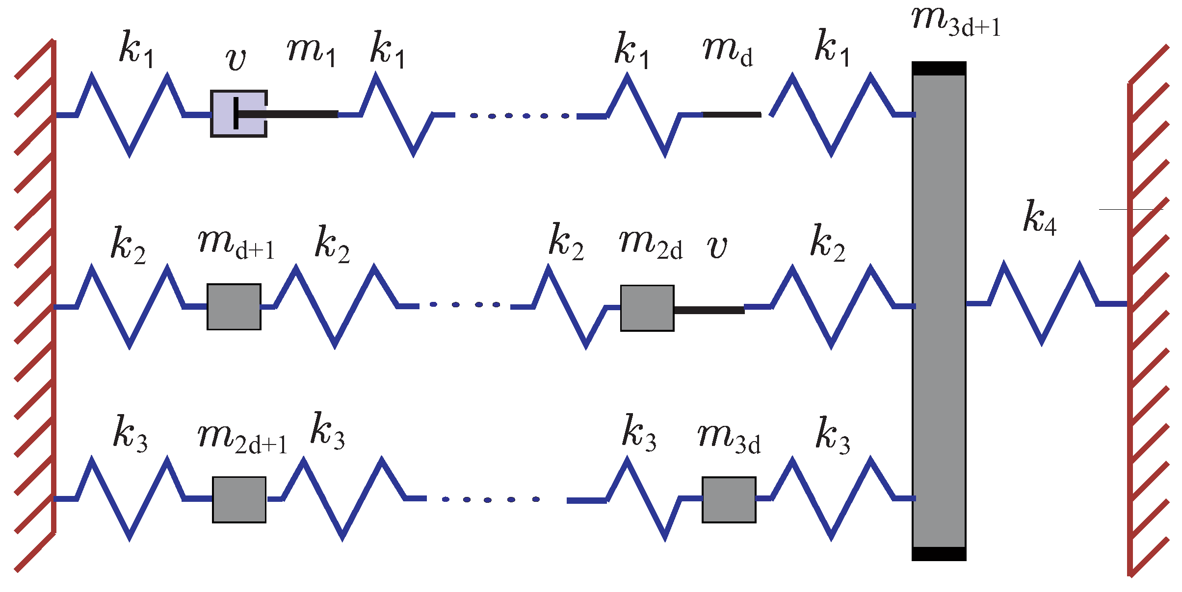
3.3. Numerical Example: Rank One

We now illustrate the results from Section 3.1 with a simple numerical example describing the mass-spring system (6)–(8).

For simplicity, we take $n=10$, all $m_i=1$, for $i=1,\dots ,n-1$ and $m_n=0$ and all $k_i=1$ for $i=1,\dots ,n-1$, yielding

$$M=\left[\begin{array}{ccccc}1& 0& & & \\ 0& 1& 0& & \\ & \ddots & \ddots & \ddots & \\ & & 0& 1& 0\\ & & & 0& 0\end{array}\right],K=\left[\begin{array}{ccccc}2& -1& & & \\ -1& 2& -1& & \\ & \ddots & \ddots & \ddots & \\ & & -1& 2& -1\\ & & & -1& 2\end{array}\right].$$

We define the damping matrix $D\doteq D(i,v)$ as a function of the viscosity parameter v and damper positions $i\in \{1,\dots ,n-1\}$, with two different structures.

$$\mathrm{Structure}1:D(i,v)=v{\mathsf{\Phi }}^{T}c{c}^T{\mathsf{\Phi }}^T,c={[e_i,1]}^T,$$

where $e_i$ denotes the i-th canonical basis vector of dimension $n-1$.

$$\mathrm{Structure}2:D(i,v)=vc{c}^T,c={[e_i,1]}^T.$$

Table 1. Optimal traces vs. damper positions.

Positions i	1	2	3	4	5	6	7	8	9
Optimal trace structure 1	$327.22$	$105.75$	$210.88$	$81.38$	$118.10$	$311.10$	$3300.1$	15,083	117,110
Optimal trace structure 2	${10}^9$	${10}^9$	$7.1768$	${10}^9$	${10}^9$	${10}^9$	${10}^9$	${10}^9$	${10}^9$

shows the optimal values of the trace function $v\to \mathrm{trace}\left(ZX\right)$, for 

$$Z\doteq f_3{f}_3^T\oplus 1\oplus f_3{f}_3^T,$$

where $f_3$ denotes the 3-th canonical basis vector of dimension $2·n-1$.

As can be seen from Table 1, it is obvious that “the best possible damping matrix” is $D=v_{opt}[e_3,1]{[e_3,1]}^T$ with optimal viscosity $v_{opt}=0.56$, which is consistent with the results from Section 3.1.

We want to emphasize that, for all other positions within structure 2, the system is extremely unstable; therefore, we add a small perturbation (of single precision order), which results in traces $O\left({10}^9\right)$.

4. The Singular Mass Case, $dim\left(\mathcal{N}\right(\mathbf{M}\left)\right)\ge \mathbf{1}$

As we described in the introduction, in this section, we consider a slightly different configuration.

Recall that we are considering a system of differential Equations (1), viz.

$$\begin{array}{c}\hfill M\ddot{x}+C\dot{x}+Kx=0,\\ \hfill x\left(0\right)=x_0,\dot{x}\left(0\right)={\dot{x}}_0,\end{array}$$

(41)

where $M,C,$ and K (mass, damping, and stiffness matrices, respectively) are real, symmetric matrices of order n.

Let $\mathsf{\Phi }=\left[\begin{array}{cc}{\mathsf{\Phi }}_0& {\mathsf{\Phi }}_{+}\end{array}\right]$ be a real non-singular matrix, such that ${\mathsf{\Phi }}_0^{T}M{\mathsf{\Phi }}_0=0_{n_0}$, ${\mathsf{\Phi }}_0^{T}M{\mathsf{\Phi }}_{+}=0_{n_0,m}$, and ${\mathsf{\Phi }}_{+}^{T}M{\mathsf{\Phi }}_{+}=I_m$, which means that we can write:

$$\begin{array}{c}\hfill {\mathsf{\Phi }}^{T}M\mathsf{\Phi }=\left[\begin{array}{cc}{0}_{n_0}& \\ & I_m\end{array}\right],{\mathsf{\Phi }}^{T}K\mathsf{\Phi }=\left[\begin{array}{cc}{\mathsf{\Omega }}_0^2& \\ & {\mathsf{\Omega }}_{+}^2\end{array}\right],\end{array}$$

(42)

where $0_{n_0}$ and ${\mathsf{\Omega }}_0$ are quadratic matrices of dimension $n_0$, with zeros and ${\omega }_1^0,\dots ,{\omega }_{n_0}^0>0$ corresponding, respectively, with zero eigenvalues in the matrix M. Further, ${\mathsf{\Omega }}_{+}=\mathrm{diag}({\omega }_1,$$\dots ,{\omega }_m)$, where $m=n-n_0$.

In addition, we assume here that $n_0\doteq dim\left(\mathcal{N}\left(M\right)\right)\ge 1$, and the damping is defined as

$$C_{in}+v·C_{ex},where{C}_{in}\doteq \alpha \mathsf{\Omega }=\alpha \left[\begin{array}{cc}{\mathsf{\Omega }}_0& \\ & {\mathsf{\Omega }}_{+}\end{array}\right].$$

Then, the damping matrix has the form

$$\begin{array}{c}\hfill D={\mathsf{\Phi }}^T\left(C_{in}+v·C_{ex}\right)\mathsf{\Phi }=\left[\begin{array}{cc}{D}_{11}& D_{12}\\ D_{12}^T& D_{22}\end{array}\right],D_{11}\in {\mathbb{R}}^{n_0,n_0},D_{22}\ne 0.\end{array}$$

Similarly to Section 2, in the first part of this section, we derive a new “linearized” system of differential equations.

First, note that all the above imply that

$$\begin{array}{c}\hfill \begin{array}{c}\hfill D_{11}{\dot{x}}_1+D_{12}{\dot{x}}_2+{\mathsf{\Omega }}_0^2{x}_0=0,\\ \hfill {\ddot{x}}_2+D_{12}^T{\dot{x}}_1+D_{22}{\dot{x}}_2+{\mathsf{\Omega }}_{+}^2{x}_{+}=0,\end{array}\end{array}$$

(43)

where $x=[x_0,x_{+}]$, and $x_0$ and $x_{+}$ are of dimension $n_0$ and m, respectively.

Let us emphasize again that the assumption $D_{12}\ne 0$ distinguishes the system under consideration from other (usually considered) systems obtained simply by deflation. If we were to have a damping such that $D_{12}=0$, then (43) would be equivalent to a system

$$\begin{array}{c}\hfill \begin{array}{c}\hfill D_{11}{\dot{x}}_1+{\mathsf{\Omega }}_0^2{x}_0=0,\\ \hfill {\ddot{x}}_2+D_{22}{\dot{x}}_2+{\mathsf{\Omega }}_{+}^2{x}_{+}=0,\end{array}\end{array}$$

of two independent equations that represent a system of differential algebraic equations and would be considered similar to [28,29].

By introducing the new variables

$$\begin{array}{c}\hfill z_1={\mathsf{\Omega }}_0{x}_0,z_2={\mathsf{\Omega }}_{+}{x}_{+},z_3={\dot{x}}_2,\end{array}$$

the system (43) becomes

$$\begin{array}{cc}\hfill {\dot{z}}_1& =-{\mathsf{\Omega }}_0{D}_{11}^{-1}{D}_{12}{z}_3-{\mathsf{\Omega }}_0{D}_{11}^{-1}{\mathsf{\Omega }}_0{z}_1\hfill \end{array}$$

(44)

$$\begin{array}{cc}\hfill {\dot{z}}_2& ={\mathsf{\Omega }}_{+}{z}_3\hfill \end{array}$$

(45)

$$\begin{array}{cc}\hfill {\dot{z}}_3& =D_{12}^T{D}_{11}^{-1}{\mathsf{\Omega }}_0{z}_1-{\mathsf{\Omega }}_{+}{z}_2+\left(D_{12}^T{D}_{22}^{-1}{D}_{12}-D_{22}\right)z_3\hfill \end{array}$$

(46)

which yields to the following linearization:

$$\begin{array}{cc}\hfill \dot{z}& =Az,\hfill \end{array}$$

(47)

$$\begin{array}{cc}\hfill A& =\left[\begin{array}{ccc}-{\mathsf{\Omega }}_0{D}_{11}^{-1}{\mathsf{\Omega }}_0& 0_{n_0,m}& -{\mathsf{\Omega }}_{+}{D}_{11}^{-1}{D}_{12}\\ 0_{m,n_0}& 0_{m,m}& {\mathsf{\Omega }}_{+}\\ D_{12}^T{D}_{11}^{-1}{\mathsf{\Omega }}_{+}& -{\mathsf{\Omega }}_{+}& D_{12}^T{D}_{11}^{-1}{D}_{12}-D_{22}\end{array}\right].\hfill \end{array}$$

(48)

We would like to emphasize that if $D_{12}=0$, then the linearization (48) would become

$$\begin{array}{cc}\hfill A_{+}& =\left[\begin{array}{cc}0& {\mathsf{\Omega }}_{+}\\ -{\mathsf{\Omega }}_{+}& -D_{22}\end{array}\right],\hfill \end{array}$$

(49)

which is the standard linearization used in many papers, such as [3,4,5,6,7].

Again, our goal is to find such an external damping $v{\mathsf{\Phi }}^T{C}_{ex}\mathsf{\Phi }$ such that

$$\mathrm{trace}\left(ZX\right)=min,$$

where X is a solution of the following Lyapunov equation:

$$A^{T}X+XA=-I,$$

(50)

where A is defined as in (48), and Z is defined as in (5).

Recall that from (36), in the case of $dim\left(\mathcal{N}\right(M\left)\right)=1$ and $\alpha =0$ (no internal damping), we have

$$\begin{array}{c}\hfill f\left(v\right)=\mathrm{trace}\left(X\right)=2·\sum _i^{k-1}{\left(X_{11}\right)}_{ii}+\sum _i^{n-1}\frac{{\omega }_n}{d_2}\frac{{\eta }_i}{{\omega }_i}{\left(d_1\right)}_i+v\frac{d_2^2}{2{\omega }_n^2}(2n-1).\end{array}$$

This and (38) imply that, for the one-dimensional singularity case, the trace function has the following form:

$$\begin{array}{c}\hfill f\left(v\right)=\frac{a_0}{v}+b_{0}v+c_0,\end{array}$$

where the constants $a_0$, $b_0$, and $c_0$ are obtained from (36) and (38).

This result is quite similar to the formula obtained in [20] for the case with non-singular mass M and rank one damping.

Unfortunately, at the moment, we do not have a similar formula for damping with a rank larger than one. Thus, we propose a new (projection) approximation for solving Lyapunov Equation (50).

Further, we take advantage of the fact that, for the solution X of the Lyapunov Equation (50) and the solution Y of the so-called dual Lyapunov equation

$$AY+Y{A}^T=-Z,$$

(51)

it holds that

$$\mathrm{trace}\left(Y\right)=\mathrm{trace}\left(ZX\right).$$

Thus, in what follows, instead of A from (48) and Z from (5), we consider the projected Lyapunov equation

$$A_p{X}_p+X_p{A_p}^T=-Z_p,$$

(52)

where

$$\begin{array}{cc}\hfill A_p& =\left[\begin{array}{ccc}-{\mathsf{\Omega }}_0{D}_{11}^{-1}{\mathsf{\Omega }}_0& 0_{12}& -{\mathsf{\Omega }}_{+}{D}_{11}^{-1}{\widehat{D}}_{12}\\ 0_{21}& 0_{22}& {\mathsf{\Omega }}_p\\ {\widehat{D}}_{12}^T{D}_{11}^{-1}{\mathsf{\Omega }}_p& -{\mathsf{\Omega }}_p& {\widehat{D}}_{12}^T{D}_{11}^{-1}{\widehat{D}}_{12}-{\widehat{D}}_{22}\end{array}\right],\hfill \end{array}$$

(53)

where ${\mathsf{\Omega }}_p$ and ${\widehat{D}}_{12}$ are p dimensional principal submatrices of ${\mathsf{\Omega }}_{+}$ and $D_{12}$, respectively. The matrix $Z_p$ is obtained as the direct sum of two p dimensional submatrices of the matrix Z. That is, if $Z=Z_1\oplus Z_2$, where $Z_1$ is $n\times n$ and $Z_2$ is $(n-n_0)\times (n-n_0)$ with $I_s$ (identity of order s) as principal submatrix, respectively, then

$$\begin{array}{c}\hfill Z_p=Z_{(p,1)}\oplus Z_{(p,2)},\end{array}$$

(54)

where $Z_{(p,1)}$ is a $(p+n_0)\times (p+n_0)$ dimensional matrix, and $Z_{(p,2)}$ is a $p\times p$ dimensional matrix, where both have $I_s$ as principal submatrix. Note that the matrices in the projected Lyapunov Equation (53) have dimensions $(2p+n_0)\times (2p+n_0)$.

We now illustrate the efficiency of the above approach. We have noticed that, in many applications, the reduced dimension is between the order of s (half the rank of the projection matrix Z from the right-hand side of the Lyapunov equation) up to two or three times s. Thus, if $s=0.1·n$ and we set $p=2·s$, this means that any direct Lyapunov solver requiring $\mathcal{O}\left(n^3\right)$ (such as Bartels–Stewart or Hammerling) requires $0.2^3\mathcal{O}\left(n^3\right)$ for the projected equations, which represents a speed increase of a factor more than 100. Obviously, the increase in speed can be even larger if the rank of the matrix Z is smaller.

To demonstrate the accuracy of the obtained approximation, we propose a simple residual error. Indeed, after solving the Lyapunov Equation (52), we have the approximate solution

$$\begin{array}{c}\hfill \begin{array}{c}pp+n_0\\ X_p=\left[\begin{array}{cc}{\left(X_p\right)}_{11}& {\left(X_p\right)}_{12}\\ {\left(X_p\right)}_{12}^T& {\left(X_p\right)}_{22}\end{array}\right].\end{array}\end{array}$$

Now, our approximation of the full dimension can be defined as

$$\begin{array}{cc}\hfill & \begin{array}{cccc}p& m-p& p& m+n_0-p\end{array}\hfill \\ \hfill \tilde{X}& =\left[\begin{array}{cccc}{\left(X_p\right)}_{11}& 0& {\left(X_p\right)}_{12}& 0\\ 0& 0& 0& 0\\ {\left(X_p\right)}_{12}^T& 0& {\left(X_p\right)}_{22}& 0\\ 0& 0& 0& 0\end{array}\right].\hfill \end{array}$$

Let A be full dimensional matrix form (52); then, the residual is simply defined as

$$\begin{array}{c}\hfill E=A\tilde{X}+\tilde{X}{A}^T+Z.\end{array}$$

(55)

The error that determines our tolerance is defined as

$$\begin{array}{c}\hfill err\doteq \frac{{\parallel E\parallel }_F}{\mathrm{trace}\left(\tilde{X}\right)}.\end{array}$$

(56)

Finally, for the optimization process, we propose an approach similar to parabolic minimization, but instead of using parabolic model functions, we propose using hyperbolic functions

$$\begin{array}{c}\hfill g\left(v\right)=\frac{a}{v}+bv+c,\end{array}$$

where $a,b$, and c are determined by a simple interpolation through the three previously determined points $v_1,v_2,$ and $v_3$. The zero of $g^{\prime }\left(v_4\right)=0$ is our first approximation for the optimal v. Now, one of the previous points $\{v_1,v_2,v_3\}$ is replaced by this new minimum $v_4$, and the process is repeated until the selected tolerance level is attained.

All of the above considerations are presented in Algorithm 1. After performing one offline step of the simultaneous diagonalization of matrices M and K as in (42),

$$\begin{array}{c}\hfill {\mathsf{\Phi }}^{T}M\mathsf{\Phi }=\left[\begin{array}{cc}{0}_{n_0}& \\ & I_m\end{array}\right],{\mathsf{\Phi }}^{T}K\mathsf{\Phi }=\left[\begin{array}{cc}{\mathsf{\Omega }}_0^2& \\ & {\mathsf{\Omega }}_{+}^2\end{array}\right],\end{array}$$

and setting (or defining) the damper “positions” (geometry),

$$D={\mathsf{\Phi }}^T\left(C_{in}+v·C_{ex}\right)\mathsf{\Phi }=D_{in}+v{D}_{ex},$$

we can present Algorithm 1.

Algorithm 1: Calculate optimal viscosity $v_{opt}$

Require:  ${\mathsf{\Omega }}_1$, ${\mathsf{\Omega }}_2$, $\{v_1,v_2,v_3\}$ - starting viscosites, Z, $D_{in}$, $D_{ex}$, $maxiter$, $tol$ Ensure:  $v_{opt}$ 1: for$i\in \{1,2,3\}$, define do 2:    $D\left(v_i\right)=D_{in}+v{D}_{ex}$ 3:    corresponding $A\left(v_i\right)$ as in (53) and $Z_p$ as in (54) 4:    define reduced dimension p, and calculate approximate solution $X_p$ of $A_p{X}_p+X_p{A_p}^T=-Z_p,$ 5:    check does $err$ from (56) satisfy $err<tol$ 6:    if $err<tol$, for $err$ from (56) then 7:      continue to 11: 8:    else     increase p and go to 4: 9:    end if 10: end for 11: For the model function $$g\left(v\right)=\frac{a}{v}+bv+c,$$ use standard linear least squares method through the points $\{g\left(v_1\right),g\left(v_2\right),g\left(v_3\right)\}$ to determine a, b, and c 12: $v_0=\sqrt{\frac{a}{b}}$ - the first approximation of optimal viscosity 13: for$k=1,\dots ,maxtier$do 14:    $v_k=v_{k-1}$ 15:    $D\left(v_k\right)=D_{in}+v\left(k\right)D_{ex}$ 16:    set $A\left(v_i\right)$ as in (53) 17:    calculate approximate solution $X_p$ of $A_p{X}_p+X_p{A_p}^T=-Z_p$ 18:    determine new set $\{v_1,v_2,v_3\}$ (leave new minimum and its “neighbors”) 19:    determine new a, b, and c for the new points $\{g\left(v_1\right),g\left(v_2\right),g\left(v_3\right)\}$ 20:    $v_k=\sqrt{\frac{a}{b}}$ - the new approximation of optimal viscosity 21:    if $$\frac{|v_k-v_{k-1}|}{|v_k|}\le tol$$ then 22:       $$v_{opt}=v_k$$ 23:      else     goto 8: 24:    end if 25: end for

5. Numerical Illustration

In this section, we illustrate the performance of Algorithm 1 on three different classes of mechanical systems, used in many papers such as [6,16], with the essential difference that we assume that the mass matrix can be singular.

Example 1.Consider the mechanical system with

$$M=\mathrm{diag}(m_1,m_2,\dots ,m_n)$$

where $m_1=\dots m_{n_0}=0$, and

$$K=\left[\begin{array}{ccccc}{k}_1& -k_1& & & \\ -k_1& k_1+k_2& -k_2& & \\ & \ddots & \ddots & \ddots & \\ & & -k_{n-2}& k_{n-2}+k_{n-1}& -k_{n-1}\\ & & & -k_{n-1}& k_{n-1}+k_n\end{array}\right].$$

Let $\mathsf{\Phi }=\left[\begin{array}{cc}{\mathsf{\Phi }}_0& {\mathsf{\Phi }}_{+}\end{array}\right]$ be a real non-singular matrix as in (42), such that

$$\begin{array}{c}\hfill {\mathsf{\Phi }}^{T}M\mathsf{\Phi }=\left[\begin{array}{cc}{0}_{n_0}& \\ & I_m\end{array}\right],{\mathsf{\Phi }}^{T}K\mathsf{\Phi }=\left[\begin{array}{cc}{\mathsf{\Omega }}_0^2& \\ & {\mathsf{\Omega }}_{+}^2\end{array}\right].\end{array}$$

As we have mentioned above, the damping matrix is defined as

$$\begin{array}{cc}\hfill D& =D_{in}+v{D}_{ex}\hfill \\ \hfill D_{in}& ={\mathsf{\Phi }}^T{C}_{in}\mathsf{\Phi },D_{ex}={\mathsf{\Phi }}^T{C}_{ex}\mathsf{\Phi }.\hfill \end{array}$$

We present results on optimal viscosities $v_{opt}$ obtained for three different configurations of $m_i$ and $k_i$, and a set of 10 prescribed positions, that is, for 10 predefined matrices $D_{ex}$.

Configuration 1.

For the first configuration, we set

$$\begin{array}{cc}\hfill n& =1000—\mathrm{dimension} \mathrm{of} \mathrm{matrices},n_0=10—\mathrm{dimension} \mathrm{of} \mathrm{null} \mathrm{subspace} \mathrm{of} M,\hfill \\ \hfill m_j& =12·j,j=n_0+1,\dots ,n,k_j=1,j=1,\dots ,n.\hfill \end{array}$$

The internal damping matrix is defined as

$$\begin{array}{cc}\hfill D_{in}& ={10}^{-4}·\mathsf{\Omega },\mathsf{\Omega }\doteq {\mathsf{\Omega }}_0\oplus {\mathsf{\Omega }}_{+}.\hfill \end{array}$$

Let ${\phi }_t$ be the t-th column of the matrix ${\mathsf{\Phi }}_{+}$. Then, the external damping matrix (which depends on positions) is defined as

$$\begin{array}{cc}\hfill D_{ex}& =\left[\begin{array}{cc}{\mathsf{\Phi }}_0& {\mathsf{\Phi }}_t\end{array}\right],{\mathsf{\Phi }}_t=\left[\begin{array}{cc}{\phi }_{21+100·t}& \dots ,{\phi }_{40+100·t}\end{array}\right],t=0,\dots ,9.\hfill \end{array}$$

This means that for the first configuration, the external damping has columns from ${\phi }_{21}$ to ${\phi }_{40}$; the second configuration has columns ${\phi }_{21}$ to ${\phi }_{40}$; and so on to the last one with columns ${\phi }_{921}$ to ${\phi }_{940}$.

It is important to emphasize that at the first $n_0$ positions, the system contains only dampers, so the first $n_0$ masses are 0.

For the matrix Z (on the right-hand side in the Lyapunov equation), we set

$$\begin{array}{c}\hfill Z=0_{n_0}\oplus Z_1\oplus Z_1,Z_1=I_s\oplus 0_{m-s},\end{array}$$

where $0_{n_0}$ is an $n_0\times n_0$ zero matrix, and $I_s$ is an identity matrix of dimension $s=100$.

The obtained results are presented in

Table 2. Optimal viscosities for Configuration 1.

Positions (t) 21:40 + 100·t	0	1	2	3	4
Optimal visc. Algorithm 1	$4.2948$	$1.7368\times {10}^1$	$30.463$	$45.934$	$61.748$
Optimal trace Algorithm 1	$5.6153\times {10}^6$	$1.1645\times {10}^6$	$1.7440\times {10}^6$	$2.5305\times {10}^6$	$3.2829\times {10}^6$
Optimal visc. fminsearch	$4.2948$	$17.368$	$30.087$	$44.850$	$59.332$
Optimal trace fminsearch	$5.6153\times {10}^6$	$1.1645\times {10}^6$	$1.7440\times {10}^6$	$2.5305\times {10}^6$	$3.2829\times {10}^6$
Rel. error (56)	$7.4424\times {10}^{-17}$	$2.7935\times {10}^{-8}$	$1.5191\times {10}^{-5}$	$1.9908\times {10}^{-5}$	$2.2599\times {10}^{-5}$
Positions(t) 21:40 + 100 ·t	5	6	7	8	9
Optimal visc. Algorithm 1	$5.3480\times {10}^1$	$4.3959\times {10}^1$	$3.8125\times {10}^1$	$3.4038\times {10}^1$	$2.9794\times {10}^1$
Optimal trace Algorithm 1	$2.9840\times {10}^6$	$2.6623\times {10}^6$	$2.4733\times {10}^6$	$2.3638\times {10}^6$	$2.1533\times {10}^6$
Optimal visc fminsearch	$5.2054\times {10}^1$	$4.3070\times {10}^1$	$3.7460\times {10}^1$	$3.3536\times {10}^1$	$2.9460\times {10}^1$
Optimal trace fminsearch	$2.9625\times {10}^6$	$2.6519\times {10}^6$	$2.4660\times {10}^6$	$2.3581\times {10}^6$	$2.1487\times {10}^6$
Rel. error (56)	$2.0869\times {10}^{-5}$	$1.8709\times {10}^{-5}$	$1.7431\times {10}^{-5}$	$1.6362\times {10}^{-5}$	$1.5729\times {10}^{-5}$

.

Configuration 2.

For the second configuration, we use bigger matrix dimensions and a different matrix K.

$$\begin{array}{cc}\hfill n& =2000—\mathrm{dimension} \mathrm{of} \mathrm{matrices},n_0=10—\mathrm{dimension} \mathrm{of} \mathrm{null} \mathrm{subspace} \mathrm{of} M,\hfill \\ \hfill m_j& =12·j,j=n_0+1,\dots ,n,k_j=1,j=1,\dots ,n.\hfill \end{array}$$

In this configuration, we consider the following stiffness matrix:

$$\begin{array}{c}\hfill \widehat{K}=\left[\begin{array}{ccccccc}4& -1& -1& & & & \\ -1& 4& -1& -1& & & \\ -1& -1& 4& -1& -1& & \\ & \ddots & \ddots & \ddots & \ddots & \ddots \\ & -1& -1& 4& -1& -1\\ & & -1& -1& 4& -1\\ & & & -1& -1& 4\end{array}\right]\end{array}$$

The internal and external damping matrices are similar to the previous case, that is

$$\begin{array}{cc}\hfill D_{in}& ={10}^{-4}·\mathsf{\Omega },\mathsf{\Omega }\doteq {\mathsf{\Omega }}_0\oplus {\mathsf{\Omega }}_{+},\hfill \end{array}$$

is defined as

$$\begin{array}{cc}\hfill D_{ex}& =\left[\begin{array}{cc}{\mathsf{\Phi }}_0& {\mathsf{\Phi }}_t\end{array}\right],{\mathsf{\Phi }}_t=\left[\begin{array}{cc}{\phi }_{21+150·t}& \dots ,{\phi }_{40+150·t}\end{array}\right],t=0,\dots ,9,\hfill \end{array}$$

where ${\phi }_t$ is the t-th column of the matrix ${\mathsf{\Phi }}_{+}$.

For the matrix Z, we use the same matrix as in the previous case defined by (54):

$$\begin{array}{c}\hfill Z=0_{n_0}\oplus Z_1\oplus Z_1,Z_1=I_s\oplus 0_{m-s},\end{array}$$

where $0_{n_0}$ is an $n_0\times n_0$ zero matrix, and $I_s$ is an identity matrix of dimension $s=100$.

The obtained results are presented in

Table 3. Optimal viscosities for Configuration 2.

Positions (t) 21:40 + 100·t	0	1	2	3	4
Optimal visc. Algorithm 1	$9.0137$	$39.209$	$7.8999\times {10}^1$	$1.2126\times {10}^2$	$1.5291\times {10}^2$
Optimal trace Algorithm 1	$9.7801\times {10}^6$	$1.4589\times {10}^6$	$2.5182\times {10}^6$	$3.4452\times {10}^6$	$3.9859\times {10}^6$
Optimal visc. fminsearch	$9.0137$	$39.209$	$7.6474\times {10}^1$	$1.13892$	$1.4135\times {10}^2$
Optimal trace fminsearch	$9.7801\times {10}^6$	$1.4589\times {10}^6$	$2.5174\times {10}^6$	$3.4136\times {10}^6$	$3.9424\times {10}^6$
Rel. error (56)	$7.0347\times {10}^{-17}$	$1.0986\times {10}^{-16}$	$1.9372\times {10}^{-5}$	$2.5991\times {10}^{-5}$	$3.1844\times {10}^{-5}$
Positions(t) 21:40 + 100·t	5	6	7	8	9
Optimal visc. Algorithm 1	$1.8644\times {10}^2$	$2.3116\times {10}^2$	$2.6915\times {10}^2$	$3.2734\times {10}^2$	$2.4521\times {10}^2$
Optimal trace Algorithm 1	$4.3150\times {10}^6$	$4.8266\times {10}^6$	$4.8698\times {10}^6$	$5.2954\times {10}^6$	$4.5854\times {10}^6$
Optimal visc fminsearch	$1.6896\times {10}^2$	$2.0028\times {10}^2$	$2.2848\times {10}^2$	$2.7213\times {10}^2$	$2.1241\times {10}^2$
Optimal trace fminsearch	$4.2718\times {10}^6$	$4.7244\times {10}^6$	$4.6841\times {10}^6$	$5.0019\times {10}^6$	$4.4533\times {10}^6$
Rel. error (56)	$3.8534\times {10}^{-5}$	$4.5229\times {10}^{-5}$	$5.0984\times {10}^{-5}$	$5.4818\times {10}^{-5}$	$4.9010\times {10}^{-5}$

.

Configuration 3.

The last case within the numerical illustrations is again an oscillator ladder with a different configuration.

This configuration is found in [6,16].

We consider the mechanical system shown in Figure 2, with $3d+1$ masses, consisting of three rows of masses with $d+1$ springs. Each row has springs of the same stiffness equal to $k_1,k_2,$ and $k_3$. On the left-hand side, rows of springs are connected to the fixed base, and on the right-hand side, they are connected to the last mass ($m_{3d+1}$), which is connected to the fixed base with a spring of stiffness $k_4$.

The mathematical model for the considered vibrational system is given by Equation (41), where the mass matrix is

$$M=\mathrm{diag}(m_1,m_2,\dots ,m_n).$$

The stiffness matrix is defined as

$$K=\left[\begin{array}{cccc}{K}_{11}& & & -{\kappa }_1\\ & K_{22}& & -{\kappa }_2\\ & & K_{33}& -{\kappa }_3\\ -{\kappa }_1^T& -{\kappa }_2^T& -{\kappa }_3^T& k_1+k_2+k_3+k_4\end{array}\right],$$

where

$$K_{ii}=k_i\left[\begin{array}{ccccc}2& -1& & & \\ -1& 2& -1& & \\ & \ddots & \ddots & \ddots & \\ & & -1& 2& -1\\ & & & -1& 2\end{array}\right],{\kappa }_i=\left[\begin{array}{c}0\\ ⋮\\ 0\\ k_i\end{array}\right],i=1,2,3.$$

In our example, we consider the following configuration:

$$\begin{array}{cc}\hfill d& =300,n=3d+1=901,\hfill \\ \hfill m_k& =0,k=1,\dots ,n_0,m_k=0.01,k=n_0+1,\dots ,d,\hfill \\ \hfill m_k& =2,k=d+1,\dots ,2·d,m_k=400,k=2·d,\dots ,3·d,m_n=100,\hfill \\ \hfill k_1& =1,k_2=2,k_3=2,k_4=5.\hfill \end{array}$$

As in the two previous cases, for the damping we take

$$\begin{array}{cc}\hfill D_{in}& ={10}^{-5}·\mathsf{\Omega },\mathsf{\Omega }\doteq {\mathsf{\Omega }}_0\oplus {\mathsf{\Omega }}_{+},\hfill \end{array}$$

which is the internal damping matrix and

$$\begin{array}{cc}\hfill D_{ex}& =\left[\begin{array}{cc}{\mathsf{\Phi }}_0& {\mathsf{\Phi }}_t\end{array}\right],{\mathsf{\Phi }}_t=\left[\begin{array}{cc}{\phi }_{21+150·t}& \dots ,{\phi }_{40+150·t}\end{array}\right],t=0,\dots ,9,\hfill \end{array}$$

for the external damping, where ${\phi }_t$ is the t-th column of the matrix ${\mathsf{\Phi }}_{+}$.

Here, as in the previous two cases, at the first $n_0$ positions (“first row”), the system contains only dampers; therefore, the first $m_i=0$, for $i=1,\dots ,n_0$.

For the matrix Z, we use the same matrix as in the previous two cases; it is defined by (54).

The obtained results are presented in

Table 4. Optimal viscosities for Configuration 3.

Positions (t) 21:40 + 100·t	0	1	2	3	4
Optimal visc. Algorithm 1	$2.0284\times {10}^{-3}$	$2.5811\times {10}^{-3}$	$2.2827\times {10}^{-3}$	$5.8067\times {10}^{-2}$	$4.5660\times {10}^{-2}$
Optimal trace Algorithm 1	$6.0377\times {10}^4$	$4.3650\times {10}^4$	$4.9078\times {10}^4$	$1.6128\times {10}^5$	$1.6156\times {10}^5$
Optimal visc. fminsearch	$2.0275\times {10}^{-3}$	$2.5790\times {10}^{-3}$	$2.2813\times {10}^{-3}$	$5.8335\times {10}^{-2}$	$4.6291\times {10}^{-2}$
Optimal trace fminsearch	$6.0377\times {10}^4$	$4.3650\times {10}^4$	$4.9078\times {10}^4$	$1.6128\times {10}^5$	$1.6156\times {10}^5$
Rel. error (56)	$2.0499\times {10}^{-4}$	$3.0910\times {10}^{-4}$	$2.7175\times {10}^{-4}$	$1.9799\times {10}^{-3}$	$1.8297\times {10}^{-3}$
Positions(t) 21:40 + 100·t	5	6	7	8	9
Optimal visc. Algorithm 1	$0.01212$	$2.0990\times {10}^3$	$9.0360\times {10}^3$	$5.2554\times {10}^3$
Optimal trace Algorithm 1	$8.8469\times {10}^4$	$7.8204\times {10}^4$	$3.3000\times {10}^5$	$1.6797\times {10}^5$
Optimal visc fminsearch	$0.01206$	$2.0175\times {10}^3$	$1.9739\times {10}^3$	$4.8508\times {10}^3$
Optimal trace fminsearch	$8.8468\times {10}^4$	$7.7174\times {10}^4$	$7.7982\times {10}^4$	$1.4775\times {10}^5$
Rel. error (56)	$1.3229\times {10}^{-3}$	$9.8193\times {10}^{-3}$	$1.1273\times {10}^{-2}$	$9.3280\times {10}^{-3}$

, where the largest projection space has a dimension of $p=350$. As a result of specified structure (the first two rows are lighter than the third one), it suffices to take $p=200$ for the positions $n_0+1,\dots ,2·n$, and $p=300$ for the positions $2·n+1,\dots ,3·n+1$.

As can be seen from Table 4, most of the obtained approximations are satisfactory, except for the positions of the external dampers from 621 to 640 (this for $t=7$). For this case, we need to increase the reduced (projected) dimension to $p=400$. This leads to the following approximations:

$$\mathrm{Opt}.\mathrm{viscosity}=2.0581\times {10}^3,\mathrm{Opt}.\mathrm{trace}=7.8030\times {10}^4,\mathrm{relative}\mathrm{error}\left(\right)=5.1034\times {10}^{-3}.$$

6. Conclusions

This paper contains two novel results for small damped oscillations described by the vector differential equation $M\ddot{x}+C\dot{x}+Kx=0$, where the mass matrix M can be singular, but standard deflation techniques cannot be applied. For example, $\mathcal{N}\left(M\right)\cap \mathcal{N}\left(C\right)=\varnothing$.

The first result is the novel formula for the solution X of the Lyapunov equation $A^{T}X+XA=-I$, where $A=A\left(v\right)$ is obtained from $M,C\left(v\right)$, and K, which are the so-called mass, damping, and stiffness matrices, respectively. These matrices are real, symmetric of order n, and $\mathrm{rank}\left(M\right)=n-1$. In addition, we assume that K is positive definite and $C\left(v\right)$ is positive semidefinite, with $\mathrm{rank}\left(C\right(v\left)\right)=1$ and no internal damping.

Using the obtained formula, we propose a novel approach for very efficiently calculating the optimal damping matrix $C_{opt}=v_{opt}{d}_{opt}{d}_{opt}^T$.

In contrast to the first part of the paper, which we refer to as the “theoretical part”, in the second part, we assumed that $dim\left(\mathcal{N}\right(M\left)\right)\ge 1$ and $C_{in}>0$ (usually a small percentage of the critical damping). We refer to this part as the “numerical part” or “numerical point of view”.

In said part, we presented a novel linearization, i.e., a novel construction of the matrix A in the Lyapunov equation $A^{T}X+XA=-I$, and a novel optimization process. The proposed optimization process computes the optimal damping $C\left(v\right)$ that minimizes a function $v\mapsto \mathrm{trace}\left(ZX\right)$, where Z is a chosen symmetric positive semidefinite matrix, using the approximation function $g\left(v\right)=c_v+\frac{a}{v}+bv$ for the trace function $f\left(v\right)\doteq \mathrm{trace}\left(ZX\right(v\left)\right)$.

The results obtained in both parts were illustrated with several corresponding numerical examples.

References

1. Cox, S.J. Designing for optimal energy absorption. II. The damped wave equation. In Control and Estimation of Distributed Parameter Systems; Birkhauser: Basel, Switzerland, 1998; pp. 103–109. [Google Scholar] [CrossRef]
2. Freitas, P.; Lancaster, P. On the optimal value of the spectral abscissa for a system of linear oscillators. SIAM J. Matrix Anal. Appl. 1999, 21, 195–208. [Google Scholar] [CrossRef]
3. Nakić, I. Optimal Damping of Vibrational Systems. Ph.D. Thesis, Fernuniversität, Hagen, Germany, 2002. [Google Scholar]
4. Brabender, K. Optimale Dämpfung von Linearen Schwingungssystemen. Ph.D. Thesis, Fernuniversität, Hagen, Germany, 1998. [Google Scholar]
5. Müller, P.C.; Gürgöze, M. Optimale Dämpfungsstärke eines viskosen Dämpfers bei einem mehrläufigen Schwingungssystem. Z. Angew. Math. Mech. 1991, 71, T60–T63. [Google Scholar]
6. Benner, P.; Tomljanović, Z.; Truhar, N. Dimension reduction for damping optimization in linear vibrating systems. Z. Angew. Math. Mech. 2011, 91, 179–191. [Google Scholar] [CrossRef]
7. Benner, P.; Tomljanović, Z.; Truhar, N. Optimal Damping of Selected Eigenfrequencies Using Dimension Reduction. Numer. Linear Algebra Appl. 2013, 20, 1–17. [Google Scholar] [CrossRef]
8. Cox, S.; Nakić, I.; Rittmann, A.; Veselić, K. Lyapunov optimization of a damped system. Syst. Control Lett. 2004, 53, 187–194. [Google Scholar] [CrossRef]
9. Cox, S.J. Designing for optimal energy absortion I: Lumped parameter systems. ASME J. Vib. Acoust. 1998, 120, 339–345. [Google Scholar] [CrossRef]
10. Truhar, N.; Tomljanović, Z.; Veselić, K. Damping optimization in mechanical systems with external force. Appl. Math. Comput. 2015, 250, 270–279. [Google Scholar] [CrossRef]
11. Veselić, K. Damped Oscillations of Linear Systems; Springer Lecture Notes in Mathematics; Springer: Berlin, Germany, 2011. [Google Scholar]
12. Fujita, K.; Moustafa, A.; Takewaki, I. Optimal placement of viscoelastic dampers and supporting members under variable critical excitations. Earthq. Struct. 2010, 1, 43–67. [Google Scholar] [CrossRef]
13. Mehrmann, V.; Schröder, C. Nonlinear eigenvalue and frequency response problems in industrial practice. J. Math. Ind. 2011, 1, 1–18. [Google Scholar] [CrossRef] [Green Version]
14. Gräbner, N.; Mehrmann, V.; Quraishi, S.; Schröder, C.; von Wagner, U. Numerical methods for parametric model reduction in the simulation of disk brake squeal. Z. Angew. Math. Mech. 2016, 96, 1388–1405. [Google Scholar] [CrossRef]
15. Kougioumtzoglou, I.; Fragkoulis, V.; Pantelous, A.; Pirrotta, A. Random vibration of linear and nonlinear structural systems with singular matrices: A frequency domain approach. J. Sound Vib. 2017, 404, 84–101. [Google Scholar] [CrossRef] [Green Version]
16. Truhar, N.; Veselić, K. An efficient method for estimating the optimal dampers’ viscosity for linear vibrating systems using Lyapunov equation. SIAM J. Matrix Anal. Appl. 2009, 31, 18–39. [Google Scholar] [CrossRef]
17. Benner, P.; Kürschner, P.; Tomljanović, Z.; Truhar, N. Semi-active damping optimization of vibrational systems using the parametric dominant pole algorithm. J. Appl. Math. Mech. 2015, 96, 604–619. [Google Scholar] [CrossRef] [Green Version]
18. Truhar, N. An efficient algorithm for damper optimization for linear vibrating systems using Lyapunov equation. J. Comput. Appl. Math. 2004, 172, 169–182. [Google Scholar] [CrossRef] [Green Version]
19. Veselić, K. On linear vibrational systems with one dimensional damping. J. Appl. Anal. 1988, 29, 1–18. [Google Scholar] [CrossRef]
20. Veselić, K. On linear vibrational systems with one dimensional damping II. Integral Equations Oper. Theory 1990, 13, 883–897. [Google Scholar] [CrossRef]
21. Truhar, N.; Veselić, K. On some properties of the Lyapunov equation for damped systems. Math. Commun. 2004, 9, 189–197. [Google Scholar]
22. Truhar, N.; Tomljanović, Z.; Puvača, M. An Efficient Approximation For Optimal Damping In Mechanical Systems. Int. J. Numer. Anal. Model. 2017, 14, 201–217. [Google Scholar]
23. Orlando, D.; Goncalves, P.B. Hybrid nonlinear control of a tall tower with a pendulum absorber. Struct. Eng. Mech. 2013, 46, 153–177. [Google Scholar] [CrossRef]
24. Viola, E.; Guidi, F. Influence of the supporting braces on the dynamic control of buildings with added viscous dampers. Struct. Control Health Monit. 2008, 16, 267–286. [Google Scholar] [CrossRef]
25. Wang, Y.; Dyke, S. Smart system design for a 3D base-isolated benchmark building. Struct. Control Health Monit. 2008, 30, 939–957. [Google Scholar] [CrossRef]
26. Benner, P.; Tomljanović, Z.; Truhar, N. Damping Optimization for Linear Vibrating Systems Using Dimension Reduction. In Proceedings of the 10th International Conference on Vibration Problems ICOVP 2011, Prague, Czech Republic, 5–8 September 2011; pp. 297–305. [Google Scholar]
27. Veselić, K.; Brabender, K.; Delinić, K. Passive control of linear systems. In Proceedings of the 1st Conference on Applied Mathematics and Computation, Dubrovnik, Croatia, 13–18 September 1999; pp. 39–68. [Google Scholar]
28. Kunkel, P.; Mehrmann, V. Damped Oscillations of Linear Systems; European Mathematical Society, Publishing House: Zürich, Switzerland, 2006. [Google Scholar]
29. Campbell, S.; Ilchmann, A.; Mehrmann, V.; Reis, T. (Eds.) Applications of DifferentialAlgebraic Equations: Examples and Benchmarks; Springer: Berlin, Germany, 2019. [Google Scholar]
Figure 1. The n-mass oscillator with one damper.
Mathematics 10 01854 g001
Figure 2. 3 d + 1 mass oscillator.
Mathematics 10 01854 g002