Swarm-Intelligence Optimization Method for Dynamic Optimization Problem

Abstract

In recent years, the vigorous rise in computational intelligence has opened up new research ideas for solving chemical dynamic optimization problems, making the application of swarm-intelligence optimization techniques more and more widespread. However, the potential for algorithms with different performances still needs to be further investigated in this context. On this premise, this paper puts forward a universal swarm-intelligence dynamic optimization framework, which transforms the infinite-dimensional dynamic optimization problem into the finite-dimensional nonlinear programming problem through control variable parameterization. In order to improve the efficiency and accuracy of dynamic optimization, an improved version of the multi-strategy enhanced sparrow search algorithm is proposed from the application side, including good-point set initialization, hybrid algorithm strategy, Lévy flight mechanism, and Student’s t-distribution model. The resulting augmented algorithm is theoretically tested on ten benchmark functions, and compared with the whale optimization algorithm, marine predators algorithm, harris hawks optimization, social group optimization, and the basic sparrow search algorithm, statistical results verify that the improved algorithm has advantages in most tests. Finally, the six algorithms are further applied to three typical dynamic optimization problems under a universal swarm-intelligence dynamic optimization framework. The proposed algorithm achieves optimal results and has higher accuracy than methods in other references.

1. Introduction

Dynamic optimization, also known as optimal control, a core part of industrial process design, directly affects the approval of multiple performance indicators such as the overall output, material loss, and efficiency improvement of the control system. It has long been an important means to maximize the value in process control of the chemical industry [1,2]. Affected by the upgrading of industry and the expansion of system scale, the established mathematical model is often full of high-dimensional, strongly nonlinear, and other complex characteristics that are difficult to deal with. Therefore, how to achieve an effective solution to this kind of dynamic optimization problem is not only a challenging but also an urgent and practical research topic. With the continuous development and deepening of optimization technology, the swarm-intelligence optimization technique, as an emerging branch, is becoming an attractive alternative to solve dynamic optimization problems [3], which is increasingly favored by academia and industry.

The earliest method applied to dynamic optimization is the indirect method [4], which has rigorous and accurate results. However, the mathematical process is often complex and difficult to implement, and there is no analytical solution [5], so it is very limited in practical application. Different from the indirect method, the direct method [6] discretizes the variables of the dynamic optimization problem into a form that can be solved by numerical methods. Among them, the CVP method [7] only discretizes the control variables. It has higher efficiency when solving the system and has become the mainstream direct method. Furthermore, the CVP method provides an effective time-domain discretization strategy, which transforms the dynamic optimization problem into a finite-dimensional NLP problem, so that the swarm-intelligence algorithm, a practical parameter optimization technique [8,9], can be used. At present, swarm-intelligence optimization techniques have attracted extensive attention in the application of various optimization problems [10,11], and have the advantages of low dependence on prior knowledge, high robustness based on population search, and no need to calculate the gradient information of the objective function.

In recent years, scholars have used swarm-intelligence algorithms to solve dynamic optimization problems, and proposed solutions including particle swarm optimization (PSO) [12], beetle antennae search (BAS) [13], ant colony optimization (ACO) [14], seagull optimization algorithm (SOA) [15], sailfish optimizer (SFO) [16], and cultural algorithm (CA) [17]. In this context, these successful application cases confirm the effectiveness of swarm-intelligence algorithms for dynamic optimization. However, in the current literature description, a universal framework of swarm-intelligence algorithms for dynamic optimization is generally ignored, which is not conducive to the further research of various algorithms with different performances, thus limiting the long-term development of swarm-intelligence dynamic optimization methods. Therefore, it is very necessary to establish a universal framework of the swarm-intelligence dynamic optimization method, which is a core topic to be solved in this paper. Furthermore, the efficiency and accuracy of solving specific problems in the existing research still need to be improved, which often requires an approach with better performance. Therefore, this paper introduces an improved version of the sparrow search algorithm (SSA) applied to dynamic optimization problems, and uses other well-known swarm-intelligence algorithms, including whale optimization algorithm (WOA) [18], marine predators algorithm (MPA) [19], harris hawks optimization (HHO) [20], and social group optimization (SGO) [21] compared under a universal swarm-intelligence dynamic optimization framework. The boosted abilities of the proposed algorithm for typical dynamic optimization problems is successfully verified.

The SSA was chosen as the base for augmentation as it has been validated as having a better optimization performance and solving ability [22,23,24,25,26] compared to PSO, grey wolf optimizer (GWO) [27], gravitational search algorithm (GSA) [28], and sine cosine algorithm (SCA) [29]. It has been successfully applied in various domains, including UAV track planning [30], density peak clustering [31], BP neural network optimization [32], robot path planning [33], and micro-grid operation [34], showing great potential. However, it is also established that the basic SSA suffers from insufficient search scope, weak resistance to local extremum, and a slow convergence rate, which needs to be further enhanced. Hybridization is a popular algorithm design approach [35], by integrating the advantages of different algorithms, a hybrid algorithm with better performance can be constructed. In this paper, SGO is introduced into the SSA optimization framework. On this basis, the good-point set, inertia weight factor, and Lévy flight are used to modify the details, and the structure of the optimization algorithm is modified by using the Student’s t-distribution model. Then, a cooperative-mutation hybrid-swarm-intelligence algorithm (CM-HSSA) is proposed to solve the dynamic optimization problem.

The main objective behind the universal swarm-intelligence dynamic optimization framework proposed in this study is to further improve the SSA from the application side, and increase the efficiency and accuracy of solving specific dynamic optimization problems. Furthermore, since the potential for algorithms with different performances under a universal swarm-intelligence dynamic optimization framework has not been investigated enough, five other well-known swarm-intelligence techniques were also implemented and tested for three typical cases. In a nutshell, the significant characteristics of our paper are listed as:

• A universal swarm-intelligence dynamic optimization method is summarized and proposed, which lays a theoretical foundation for subsequent research on using the swarm-intelligence technique to solve dynamic optimization problems.
• A novel modified SSA is implemented from the application side and utilized to improve the efficiency and accuracy of typical dynamic optimization problems.
• Other well-known swarm-intelligence techniques for dynamic optimization are further investigated under a universal optimization framework.

The rest of the paper is organized in the following manner. Section 2 describes the fundamental methods used (the CVP method and a universal swarm-intelligence dynamic optimization method). Section 3 introduces the modified version of the algorithm as well as the original one and tests other algorithms on benchmark functions. Section 4 deals with the optimization of typical dynamic optimization problems with six algorithms under a universal swarm-intelligence dynamic optimization framework. Finally, Section 5 summarizes some conclusions and prospects for future work.

2. Preliminaries

In this section, firstly, the standard mathematical model of the dynamic optimization problem is introduced. Secondly, the basic principle of the CVP strategy is introduced, and then a universal swarm-intelligence dynamic optimization framework is summarized and proposed. In particular, the general implementation scheme and flow chart of this method are given.

2.1. Dynamic Optimization Problem Description

Generally, dynamic optimization problems are common in the control systems of industrial processes and widely exist in the chemical industry. The research object is mainly aimed at dynamic time-varying systems [36]. The established mathematical model is often described in the form of a differential–algebraic equation (DAE), which contains constraints and an objective function. Therefore, the essence of solving the dynamic optimization problem is to apply the control effect to the variables in the model and then select the appropriate optimization scheme to make the performance index in the process reach the best state. The mathematical model of a typical dynamic optimization problem can be described as follows:

$$\begin{array}{c}\min J=\Phi [x(t_f)]+{\int }_{t_0}^{t_f}L[x(t),u(t),t]dt\\ s.t.\{\begin{array}{l}\frac{dx}{dt}=f[x(t),u(t),t]\\ x(t_0)=x_0\\ u_{lb}\le u(t)\le u_{ub}\\ t\in [t_0,t_f]\end{array}\end{array}$$

(1)

where $J$ is the objective function, also known as the performance index, which is composed of the final value term $\Phi [x(t_f)]$ at the process termination time $t_f$ and the integral term ${\int }_{t_0}^{t_f}L[x(t),u(t),t]dt$ existing on the whole time period $[t_0,t_f]$, $u(t)={[u_1(t),u_2(t),\cdots ,u_m(t)]}^T$ is the m-dimensional control variable, and constrained by the upper boundary $u_{ub}$ and the lower boundary $u_{lb}$, $x(t)={[x_1(t),x_2(t),\cdots ,x_n(t)]}^T$ is the n-dimensional state variable. Therefore, Equation (1) can be briefly described as looking for the control variable $u(t)$ that makes the target $J$ obtain the optimal value under the condition of the initial state $x(t_0)=x_0$, and the value of $u(t)$ should meet the requirements of the feasible region.

2.2. CVP Strategy

As the mainstream numerical calculation method in the direct solution, the principle of the CVP method is to use the basic function with finite parameters to approach the control effect. Specifically, the strategy first discretizes the time domain ($[t_0,t_f]$) into $NE$ sub-interval ($[t_{k-1},t_k] (k=1,2,\cdots ,NE)$), that is, $t_0\le t_1\le \cdots \le t_{N-1}\le t_{NE}=t_f$, and further uses the basis function to approximate the components on each sub-interval, then $u(t)$ can be expressed as the cumulative sum of each component on the whole $[t_0,t_f]$:

$$u(t)={\displaystyle \sum _{k=1}^{NE}{\sigma }_j^k(t)}\hspace{1em}j=1,2,\cdots ,m\hspace{1em}k=1,2,\cdots ,NE$$

(2)

where ${\sigma }_j^k(t)$ is the linear combination of the basic function of the known structure of each component ($u_j(t)$) in the time interval ($[t_{k-1},t_k]$), which is determined by limited parameters. The mathematical model of the optimization problem transformed by the CVP method can be described as:

$$\begin{array}{c}\min \tilde{J}=\phi [\sigma (t)]\\ s.t.u_{lb}\le {\displaystyle \sum _{k=1}^{NE}{\sigma }^k(t)\le u_{ub}}\end{array}$$

(3)

where $\sigma (t)={[{\sigma }^1(t),{\sigma }^2(t),\cdots ,{\sigma }^{NE}(t)]}^T$ is the parameter vector to be optimized. Therefore, the CVP method provides an effective transformation method, and an infinite-dimensional dynamic optimization problem is transformed into a finite-dimensional static optimization problem with a finite number of parameters.

2.3. Swarm-Intelligence Dynamic Optimization Method Based on CVP Strategy

For dynamic optimization problems, after CVP processing, the control variables, state variables, objective functions, and constraints of the system are all determined by the parameter vector, thus forming the NLP problem which can be solved by the swarm-intelligent optimization algorithm. Depending on the type of basis function, the approximation effect is also different. As the most important type of basis function, the piecewise constant approximation strategy is the most reasonable choice from theoretical analysis to practical calculation, and has the characteristics of simplicity and effectiveness. Figure 1 shows the control curve approximated by piecewise constant when NE = 7.

In particular, different from the traditional deterministic optimization algorithm based on gradient, the swarm-intelligence optimization algorithm established by randomness generally does not need to calculate the gradient information about the objective function, so the relevant gradient calculation process is not included in the solution structure. The calculation steps of the swarm-intelligence dynamic optimization method based on the CVP strategy are as follows. Figure 2 shows the calculation framework of this method.

(1)

Through the CVP strategy, $u(t)$ is transformed into $\sigma (t)$, and the dynamic optimization problem shown in Equation (1) is transformed into the static optimization problem form shown in Equation (3).

(2)

Set relevant parameters, such as population size, the maximum number of iterations, and algorithm parameters.

(3)

Initialize the population.

(4)

Evaluate and sort the fitness values of individuals in the population and record the current optimal value.

(5)

According to the evolution strategy of the algorithm, a new population is generated.

(6)

Compare the fitness value of the new solution and replace it if it is better than the current value.

(7)

Determine whether the current condition meets the stop criterion; if so, terminate the algorithm and output the optimal solution. Otherwise, return to (4) and continue to execute, and set t = t + 1.

3. Mathematical Models and Algorithms

This beginning of the section introduces the basic implementation of the SSA algorithm, followed by a discussion about the known and observed flaws and drawbacks of the original version, and a detailed description of the proposed modified algorithm that is devised to specifically overcome these flaws of the original algorithm is provided. In the end, ten groups of benchmark functions are used to test the performance of the proposed algorithm, WOA, MPA, HHO, SSA, and SGO.

3.1. Sparrow Search Algorithm

The mathematical model of SSA mainly refers to the foraging habits of sparrows, idealizes the individual behavior in the population, formulates the corresponding iterative rules, and divides the individual into two roles of producers and scroungers in each generation according to the fitness value. In addition, SSA also designed an early warning process, which is to randomly select some individuals in the population called scouters, and update their locations in each iteration. Finally, it searches for the global optimal solution through a certain number of iterations.

The locations of producers are updated as follows:

$$X_i^{t+1}=\{\begin{array}{l}{X}_i^t\cdot \exp \left(-\frac{i}{\alpha \cdot Ite{r}_{\max }}\right),{{\displaystyle }}^{}\hspace{1em}{R}_2<ST\\ X_i^t+Q\cdot L,\hspace{1em}\hspace{1em}\hspace{1em}\hspace{1em}\hspace{1em}{R}_2\ge ST\end{array}$$

(4)

where t represents the current iteration, $Ite{r}_{\max }$ is the maximum number of iterations, $\alpha$ is a random number in the range of (0, 1], $Q$ is a random number subject to normal distribution, $L$ is a $1\times D$ matrix with each element value of 1, $R_2(R_2\in [0,1])$ and $ST(ST\in [0.5,1])$ represent the alarm value and safety threshold, respectively. It can be seen from Equation (4) that their values determine the update mode of producers

The locations of scroungers are updated as follows:

$$X_i^{t+1}=\{\begin{array}{l}Q\cdot \exp \left(\frac{X_{worst}^t-X_i^t}{i^2}\right),\hspace{1em}\hspace{1em}\hspace{1em}i>n/2\\ X_p^t+\left|X_i^t-X_p^t\right|\cdot A^{+}\cdot L,\hspace{1em}otherwise\end{array}$$

(5)

where $n$ represents the number of sparrows, $X_p$ is the best foraging location occupied by the current producers, $X_{worst}^t$ is the current worst foraging location, is a $A$ matrix with element values of 1 or −1, and $A^{+}=A^T{(A{A}^T)}^{-1}$. $Q$ and $L$ are the same as in Equation (4).

The locations of scouters are updated as follows:

$$X_i^{t+1}=\{\begin{array}{l}{X}_{best}^t+\beta \cdot \left|X_i^t-X_{best}^t\right|, f_i>f_g\\ X_i^t+K\cdot \left(\frac{\left|X_i^t-X_{worst}^t\right|}{\left(f_i-f_w\right)+\epsilon }\right), f_i=f_g\end{array}$$

(6)

where $f_i$ is the individual fitness value of scouters, $f_g$ represents the global optimal fitness value, $X_{best}^t$ is the global optimal foraging location, $\beta$ is $K$ are step control parameters, and $\epsilon$ is a minimal constant to avoid the denominator being zero.

The flowchart of SSA is shown in Figure 3.

3.2. Multi-Strategy Improved Hybrid Swarm-Intelligence Optimization Algorithm

3.2.1. Good-Point Set Theory

Previous studies have shown that the impact of the distribution of the initial population on swarm-intelligence algorithms cannot be ignored [9]. To improve the uniformity of the initial population search in solution space, scholars mostly use a chaotic map strategy to solve this problem. At present, the commonly used chaotic map models include circle map [37], tent map [38], piecewise map [39], cat map [40], logistic map [41], and Gauss map [42]. However, although this initialization method based on chaotic mapping has achieved some results, it still has considerable randomness, so it cannot effectively ensure the search breadth of the initial population.

To solve the above problems, this paper applies the good-point set theory [43] to the initial population stage. Its construction principle is: set $G_s$ be the unit cube in s-dimensional Euclidean space, and if $r\in G_s$, the shape is as follows:

$$P_n(k)=\left\{\left(\left\{r_1^{(n)}\cdot k\right\},\left\{r_2^{(n)}\cdot k\right\},\cdots ,\left\{r_s^{(n)}\cdot k\right\}\right),1\le k\le n\right\}$$

(7)

If the deviation $\phi (n)=C(r,\epsilon )n^{-1+\epsilon }$ is satisfied, where $C(r,\epsilon )$ is the constant only related to $r$ and $\epsilon (\epsilon >0)$, then $P_n(k)$ is the good-point set and $r$ is the good point. $\left\{r_s^{(n)}\cdot k\right\}$ indicates the decimal part, $n$ is the number of samples, and we set $r=\{2\cos (2\pi k/p),1\le k\le s\}$ and $p$ as the minimum prime number satisfying $(p-3)\ge s$. Mapping the good points of $G_s$ to the search space is:

$$X_{i,j}=\left\{r_j^{(i)}\cdot k\right\}\cdot (u{b}_j-l{b}_j)+l{b}_j$$

(8)

with the same number of points, a consistent distribution effect can be obtained each time using the good-point set to initialize the population. Because the construction of the good-point set is independent of the dimension of the sample, it plays a better role in solving high-dimensional problems. Through calculation and analysis, the deviation of the good-point set is $O(n^{-1+\epsilon })$, while the deviation of the random method is $O(n^{-1/2}{(\log \log n)}^{1/2})$. Compared with the random method, the deviation of the good-point set is reduced to the square-root level. Therefore, the good-point set theory provides a stable and effective uniform point selection strategy for population initialization.

To intuitively compare the two initialization methods, the population distribution generated by the random method and good-point set method when $N=100$ on $[0,1]$ is provided in Figure 4. In addition, we further compared the six commonly used chaotic maps mentioned above with the good-point set method. Considering the randomness of chaotic maps, we carried out 10 experiments, and the average value distributions of each method when $N=100$ are shown in Figure 5.

3.2.2. Hybrid Algorithm Strategy

In SSA, the producers represent the sparrows with better fitness in the population, and have the function of guiding other individuals to move to the best foraging location. Therefore, the location update process of the producers will closely affect the optimization ability of SSA. According to Equation (4), the producers have two ways of updating their locations. When $R_2\ge ST$, the individuals will move randomly near the current locations according to the normal distribution; when $R_2<ST$, the update of the locations is affected by Equation (9):

$$f(x)=\exp (-\frac{x}{\alpha \cdot Ite{r}_{\max }})$$

(9)

when $Ite{r}_{\max }=1000$, $N=1000$, $D=1$ and $\alpha =1$, the value distribution of the producers is shown in Figure 6. It can be seen that the search scope of producers shows an obvious reduction trend with iterations, and finally decreases to less than half of the initial range, all concentrated in the range of 0 to 0.4. The reduction of the search range is bound to reduce the population diversity in the optimization process, resulting in a search blind area, which increases the risk of SSA falling into the local extremum in the later stages of the iteration.

To improve the deficiency of the location update strategy of the producers, we decided to introduce the improvement phase of SGO to replace Equation (4). The mathematical model of the improvement phase of SGO is as follows:

$$X_i^{t+1}=c\cdot X_i^t+r\cdot (X_{best}^t-X_i^t)$$

(10)

where $t$ represents the current number of iterations, $X_i^t$ and $X_{best}^t$ are the current individual location and the global optimal individual location, respectively, $c\in (0,1)$ is the self-reflection parameter, which is 0.2 in the original reference [15], and $r$ is a random number satisfying uniform distribution from $[0,1]$. It can be seen that the location update will be guided by the current optimal individual, which is conducive to improving the global exploration ability and the convergence rate of the algorithm in the initial stage. However, as the self-reflection parameter, the constant attribute of $c$ leads to an invariance dependence on the location information with iterations. We change $c$ into an inertia weight factor whose value changes dynamically [44], as shown in Equation (11):

$$c^t=\frac{c_s(c_s-c_e)(Ite{r}_{\max }-t)}{Ite{r}_{\max }}$$

(11)

where $c^t$ represents the inertia weight factor, $c_s$ and $c_e$ represent the adjustment parameters, $c_s=0.9$. and $c_s=0.4$ are set, respectively. Therefore, by introducing $c^t$, the adaptive regulation of the participation degree of its location information is achieved. The decreasing characteristic of $c^t$ makes the algorithm maintain a good global exploration ability at the early stage of iteration and helps the algorithm have a more effective local development ability at the later stage of iteration. Figure 7 describes the changing trend of $c^t$ with iterations. The new producers’ update strategy is shown in Equation (12):

$$X_i^{t+1}=c^t\cdot X_i^t+r\cdot (X_{best}^t-X_i^t)$$

(12)

where $c^t$ is the inertia weight factor, $X_i^{t+1}$, $X_i^t$ and $X_{best}^t$ are the next-generation location, current location, and current optimal location of the producer, respectively.

3.2.3. Stagnation Disturbance Strategy Based on Lévy Flight

When the iteration proceeds to a certain extent, affected by the local extremum, the update range of the producers will become smaller or move only near the current region. At this time, more and more producers will change into scroungers, which indicates that there is no solution in the nearby region, causing the algorithm to stagnate.

Lévy flight is a random walk. Studies have shown that the movement patterns of many animals can be described by it [45]. Since the generation of its step is affected by the heavy-tailed distribution, there will be a jump performance with a large span during the random walk. Therefore, Lévy flight is applied to the update of individuals as a disturbance, which will enable the search of the algorithm to enter a broader area and improve the ability of global exploration. Furthermore, to further illustrate that Lévy flight can adapt to larger-scale search, Brownian motion trajectory and Lévy flight trajectory simulated by the Mantegna method [46] are revealed in Figure 8.

The calculation method of Lévy flight in this paper is as follows [47]:

$$Lévy(x)=0.01\times \frac{{\theta }_1\cdot \sigma }{{\left|{\theta }_2\right|}^{\frac{1}{\beta }}}$$

(13)

where ${\theta }_1$ and ${\theta }_2$ are parameters subject to normal distribution, $\beta$ is a constant, which is taken as 1.5 in this paper, and $\sigma$ is calculated as follows:

$$\sigma ={\left[\frac{\mathsf{\Gamma }(1+\beta )\cdot \sin (\pi \cdot \beta /2)}{\mathsf{\Gamma }((1+\beta )/2)\cdot \beta \cdot 2^{(\beta -1)/2}}\right]}^{\frac{1}{\beta }}$$

(14)

where $\mathsf{\Gamma }(x)$ is the $gamma$ function and $\mathsf{\Gamma }(x)=(x-1)!$ and x belongs to the set of natural numbers.

The new scroungers’ update strategy is shown in Equation (16):

$$X_i^{t+1}=\{\begin{array}{l}{X}_i^t+X_i^t\cdot Lévy(d),\hspace{1em}\hspace{1em}\hspace{1em}\hspace{1em}i>n/2\\ X_p^t+\left|X_i^t-X_p^t\right|\cdot A^{+}\cdot L,\hspace{1em}otherwise\end{array}$$

(15)

where $X_i^{t+1}$, $X_i^t$ and $X_p^t$ are the next-generation location, current location, and current optimal location of the scrounger, respectively, and $d$ represents the dimension of the location vector.

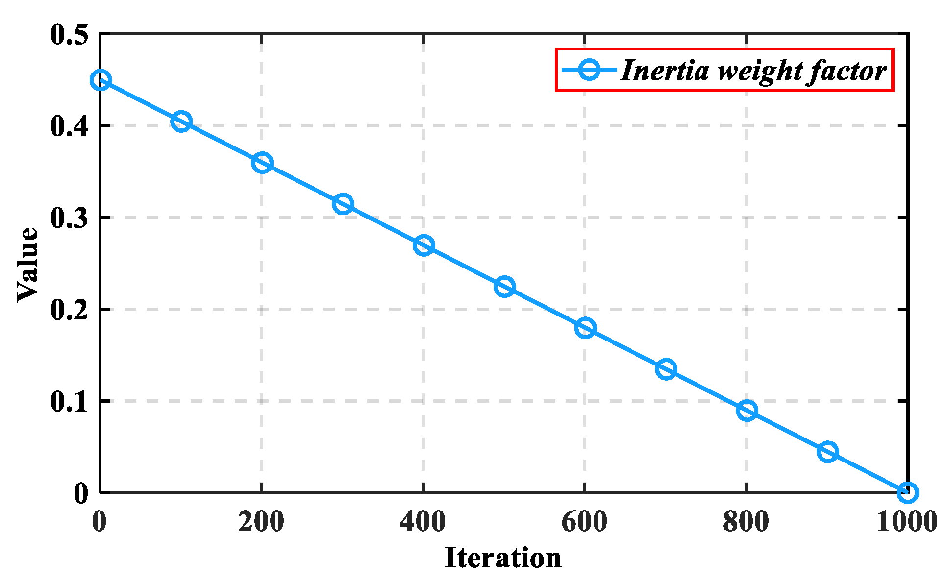
3.2.4. Early Warning Process Based on Student’s t-Distribution Mutation Factor

According to Equation (6), the update of the early warning process is related to the fitness value of the individual. When $f_i>f_g$, the individual will move towards the current optimal location, When $f_i=f_g$, the individual will move randomly in the area near itself, and the distance is related to the current worst location and the worst fitness value. Therefore, the early warning process of SSA is essentially the furthest disturbance to the population location after the iteration of producers and scroungers.

Student’s t-distribution is an important distribution type. Its curved shape is related to the change in degrees of freedom $n$. When $n=1$, t-distribution is Cauchy distribution; when $n\to \infty$, t-distribution is Gaussian distribution, that is, Cauchy distribution and Gaussian distribution are two special cases of Student’s t-distribution.

In this paper, the degrees of freedom for t-distribution are taken from the current iteration, and a mutation factor based on the Student’s t-distribution that changes with iterations can be obtained. This is applied to scouters in the early warning process as a random disturbance. The mathematical model of the new early warning process is shown in Equation (16).

$$X_i^{t+1}=X_p^t+X_p^t\cdot trnd(t)$$

(16)

where $trnd(t)$ is the t-distribution mutation factor with the current iteration as the degree of freedom, and $X_i^{t+1}$ and $X_p^t$ are the next-generation location and current optimal location of the scouter, respectively. Moreover, the mutation factor combines the advantages of Cauchy distribution and Gaussian distribution and generates different disturbance ranges through changing degrees of freedom, which can effectively balance the global exploration ability and local development ability of the algorithm. The improved algorithm based on the t-distribution mutation factor is defined as the collaborative-mutation hybrid sparrow search algorithm (CM-HSSA). The pseudo-code of CM-HSSA is shown in Algorithm 1:

Algorithm 1: The framework of CM-HSSA

Input: Max_Iter: the maximum iteration; N: the population size; PD: the proportion of producers; SD: the proportion of early warning sparrows; cs, ce: the inertia weight adjustment parameters. Output:Xbest: the optimal individual location; fg: the fitness value of the optimal individual. /* Initialization*/ 1. for i = 1 to N do 2.  for j = 1 to d do 3.   Initialize the location of N sparrows using equation (8); 4.  end for 5. end for /*Iterative search*/ 6. Calculate the fitness value and record the current optimal individual; 7. for (t < Max_iter) 8.  for i = 1 to PD*N do 9.   Update the location of producers according to equation (12); 10.  end for 11.  for i = PD*N + 1 to N do 12.   Update the location of scroungers according to equation (15); 13.  end for 14.  for i = 1 to SD*N do 15.   Update the location of early warning sparrows according to equation (16); 16.  end for 17.  Evaluate the fitness value of the new location and update if it is better; 18. end for /*Algorithm terminated*/ 19. ReturnXbest, fg

3.3. Benchmark Function Experiments

This section provides ten groups of classical benchmark functions to test the optimization performance of six algorithms, including four unimodal functions with only one global optimal value and five multimodal functions with multiple local extremums. $F_1–F_8$ are 30 dimensions and $F_9–F_{10}$ are 2 dimensions.

Table 1. Information on benchmark functions.

Benchmark Function	Formula	Range	Opt
Sphere Model	$F_1(x)={\displaystyle \sum _{i=1}^n{x}_i{}^2}$	[−100, 100]	0
Schwefel’s problem 2.22	$F_2(x)={\displaystyle \sum _{i=1}^n\left|x_i\right|+}{\displaystyle \prod _{i=1}^n\left|x_i\right|}$	[−10, 10]	0
Schwefel’s problem 1.2	$F_3(x)={{\displaystyle \sum _{i=1}^n\left({\displaystyle \sum _{j=1}^i{x}_j}\right)}}^2$	[−100, 100]	0
Schwefel’s problem 2.21	$F_4(x)={\max }_i\left\{\left|x_i\right|,1\le i\le n\right\}$	[−100, 100]	0
Generalized Schwefel’s problem 2.26	$F_5(x)={\displaystyle \sum _{i=1}^n-x_i\sin \sqrt{\left|x_i\right|}}$	[−500, 500]	−4.18.9829D
Generalized Rastrigin’s Function	$F_6(x)={\displaystyle \sum _{i=1}^n[x_i^2-10\cos (2\pi x_i)+10]}$	[−5.12, 5.12]	0
Ackley’s Function	$F_7(x)=-20\exp \left(-0.2\sqrt{\frac{1}{n}{\displaystyle \sum _{i=1}^n{x}_i{}^2}}\right)-\exp \left(\frac{1}{n}{\displaystyle \sum _{i=1}^n\cos \left(2\pi x_i\right)}\right)+20+e$	[−32, 32]	0
Generalized Griewank Function	$F_8(x)=\frac{1}{4000}{\displaystyle \sum _{i=1}^n{x}_i^2-{\displaystyle \prod _{i=1}^n\cos \frac{x_i}{\sqrt{i}}+1}}$	[−600, 600]	0
Branin Function	$F_9(x)={\left(x_2-\frac{5.1}{4{\pi }^2}{x}^2+\frac{5}{\pi }{x}_1-6\right)}^2+10\left(1-\frac{1}{8\pi }\right)\cos x_1+10$	[−5, 5]	0.398
Goldstein–Price Function	$\begin{array}{c}{F}_{10}(x)=[1+{(x_1+x_2+1)}^2(19-14x_1+3x_1^2-14x_2+6x_1{x}_2+3x_2^2)]\times \\ [30+{(2x_1-3x_2)}^2(18-32x_1+12x_1^2+48x_2-36x_1{x}_2+27x_2^2)]\end{array}$	[−2, 2]	3

gives the relevant information on these benchmark functions. The range represents the search scope, Opt represents the theoretical optimal value and D represents the dimension of the problem. Among them, $F_1–F_4$ can test the convergence rate, accuracy, and local development ability, while $F_5–F_{10}$ can test the anti-local extremum ability and global exploration ability.

3.3.1. Parameter Settings

To verify the significance of the improvement, we compared the optimization effects of WOA, MPA, HHO, SSA, SGO, and CM-HSSA on benchmark functions. To ensure the objectivity of the experiments, the population is set to 30 and the maximum iteration is 100. The specific parameter settings of each algorithm are as follows. For WOA, the logarithmic spiral shape parameter $b=1$. For MPA, the fish aggregating device $FADs=0.2$. For HHO, the prey energy factor $E$ is a random number between $(-1,1)$. For SSA, the safety threshold $ST=0.8$, the proportion of producers $PD=0.2$, and the proportion of scouters $SD=0.1$. For SGO, the self-reflection parameter $c=0.2$. For CM-HSSA, the proportion of producers $PD=0.2$, the proportion of scouters $SD=0.1$, and weight adjustment parameters $c_s=0.9$ and $c_e=0.4$. It is worth noting that the above parameters are taken from the original references. The values of these artificially set parameters are obtained based on experience, which can maximize the optimization performance of the algorithms.

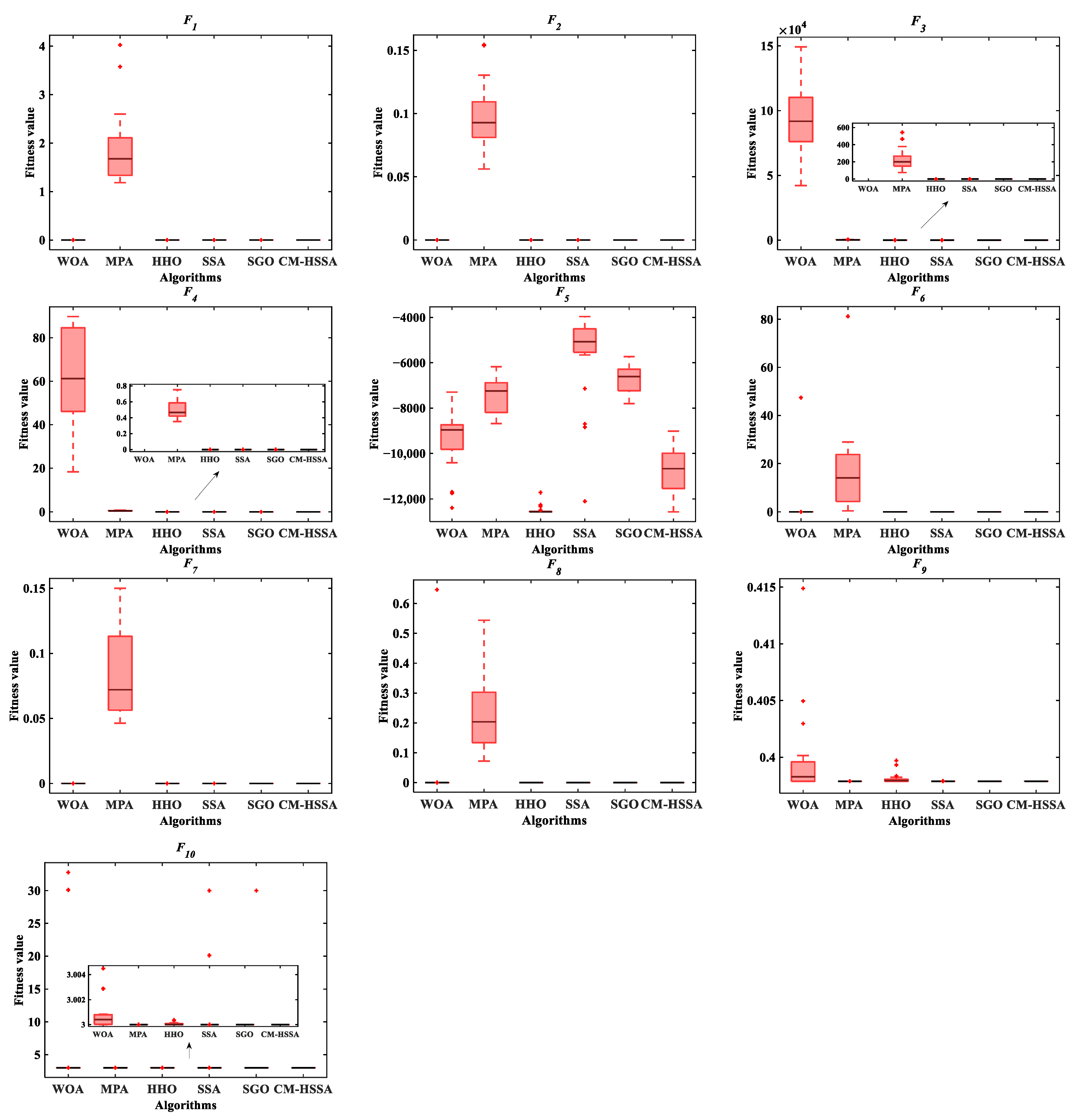
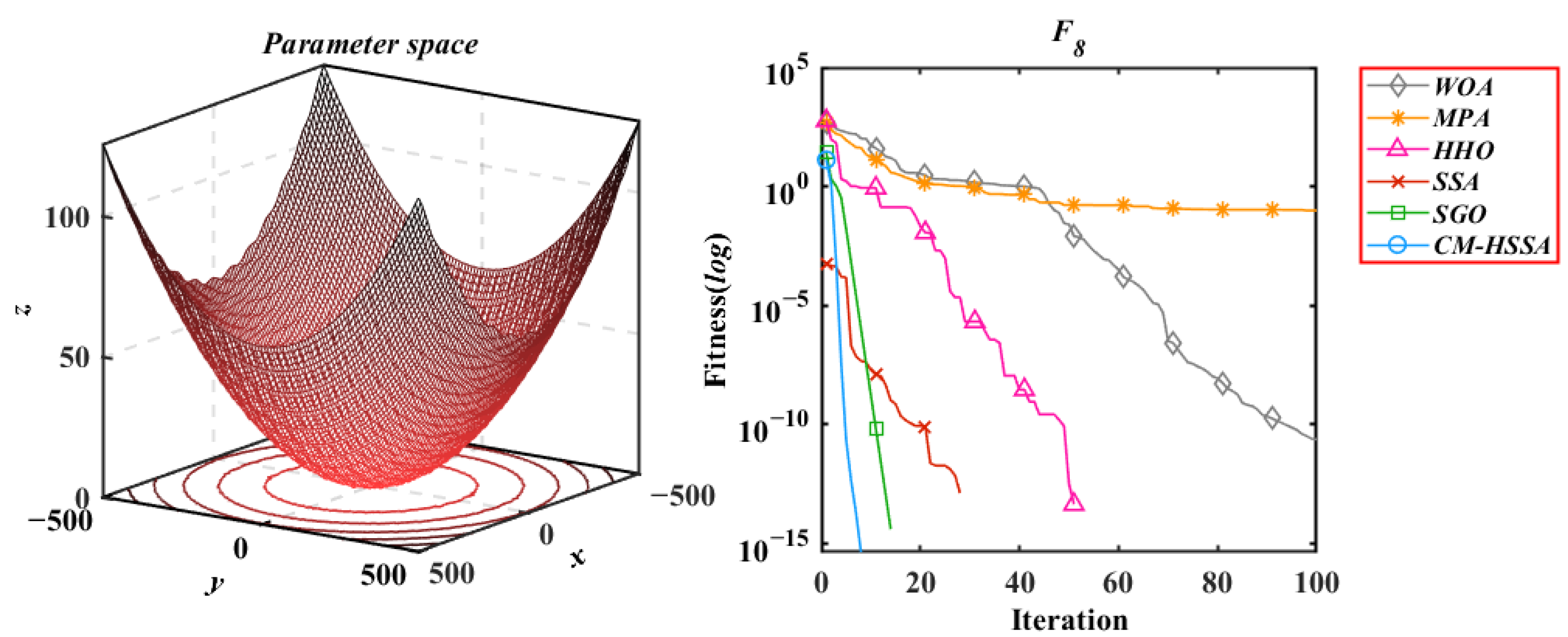
3.3.2. Statistical Result Comparison

To ensure the fairness of the experiments, each algorithm runs 20 times independently, and the mean value, standard deviation, and average calculation time are recorded. Among them, the mean value reflects the optimization accuracy, the standard deviation reflects the robustness, and TIC/TOC is used to calculate the running time of each algorithm. Through the experimental results listed in

Table 2. Experimental results of six algorithms.

Function	Result	WOA	MPA	HHO	SSA	SGO	CM-HSSA
$F_1$	Mean	3.5706 × 10−10	1.9437	1.3052 × 10−20	2.9595 × 10−33	4.3773 × 10−135	0
	Std.	7.1180 × 10−10	1.0336	5.8268 × 10−20	1.3235 × 10−33	2.9367 × 10−136	0
	TIC/TOC	0.075297	0.260806	0.122167	0.098561	0.121907	0.102957
$F_2$	Mean	9.7066 × 10−9	9.6357 × 10−2	4.3809 × 10−13	2.0208 × 10−21	1.5103 × 10−68	0
	Std.	2.1815 × 10−8	3.3799 × 10−2	1.0991 × 10−12	8.9306 × 10−21	1.6423 × 10−69	0
	TIC/TOC	0.060907	0.197253	0.121605	0.090216	0.127647	0.096940
$F_3$	Mean	9.8067 × 104	2.1566 × 102	1.8472 × 10−13	4.1637 × 10−33	2.2632 × 10−135	0
	Std.	2.8622 × 104	1.8756 × 102	8.2479 × 10−13	1.8621 × 10−32	9.9703 × 10−136	0
	TIC/TOC	0.098011	0.306055	0.232791	0.116329	0.246341	0.148943
$F_4$	Mean	5.6341 × 101	4.5856 × 10−1	3.6428 × 10−13	3.9747 × 10−21	1.0950 × 10−68	0
	Std.	2.8796 × 101	1.0924 × 10−1	6.1075 × 10−13	1.7745 × 10−20	5.3688 × 10−70	0
	TIC/TOC	0.060370	0.203315	0.113611	0.106351	0.126110	0.117772
$F_5$	Mean	−8.6688 × 103	−7.2695 × 103	−1.2356 × 104	−6.2868 × 103	−6.9435 × 103	−1.06 × 104
	Std.	1.0522 × 103	4.7419 × 102	7.9240 × 102	1.6650 × 103	6.5873 × 102	7.8299 × 102
	TIC/TOC	0.067170	0.251228	0.157786	0.079425	0.111361	0.098025
$F_6$	Mean	1.2998 × 10−8	8.6017	0	0	0	0
	Std.	5.3053 × 10−8	7.2342	0	0	0	0
	TIC/TOC	0.060027	0.217248	0.177083	0.076583	0.130681	0.106733
$F_7$	Mean	3.7669 × 10−7	8.9223 × 10−2	7.3576 × 10−12	1.0658 × 10−15	8.8818 × 10−16	8.8818 × 10−16
	Std.	5.5884 × 10−7	2.8663 × 10−2	2.2196 × 10−12	7.9441 × 10−16	0	0
	TIC/TOC	0.071849	0.177886	0.127309	0.079305	0.122893	0.098612
$F_8$	Mean	9.1942 × 10−1	2.7695 × 10−1	0	0	0	0
	Std.	2.8307 × 10−1	1.4355 × 10−1	0	0	0	0
	TIC/TOC	0.073628	0.198219	0.159379	0.077422	0.131028	0.115157
$F_9$	Mean	4.0011 × 10−1	3.9789 × 10−1	3.9853 × 10−1	3.9789 × 10−1	3.9789 × 10−1	3.9789 × 10−1
	Std.	3.7678 × 10−3	5.0943 × 10−11	1.1419 × 10−3	6.3089 × 10−7	2.3781 × 10−8	0
	TIC/TOC	0.051275	0.173310	0.137616	0.098129	0.096289	0.083473
$F_{10}$	Mean	8.4292	3.0201	3.0231	3.0023	3.0001	3.0000
	Std.	1.1139 × 101	1.8833 × 10−10	1.4497 × 10−4	2.7527 × 10−7	1.9782 × 10−7	2.2017 × 10−15
	TIC/TOC	0.056070	0.183948	0.155738	0.071500	0.107347	0.081171

, we can see the different optimization performances of the algorithms.

The simulation software used in experiments was MATLAB R2018b. It is worth mentioning that iterations are generally positively correlated with the accuracy, while the maximum iteration set in this paper is 100, which can better reflect the optimization performance of the algorithms in short iterations. According to Table 2, CM-HSSA can obtain the stable optimal convergence accuracy for unimodal functions $F_1-F_4$, and the optimization performance is better than other algorithms. For multimodal functions, HHO has the highest accuracy on $F_5$, followed by CM-HSSA. The mean value of the two algorithms has reached the level of −1 × 10⁴, which is higher than other algorithms. For $F_6$ and $F_8$, CM-HSSA, HHO, SSA, and SGO can obtain the best optimization accuracy. Although their convergence behavior is different, they all successfully find the global optimal solution in the limited iteration. For $F_7$, $F_9$, and $F_{10}$, CM-HSSA has the highest accuracy and the smallest standard deviation, which is better than other algorithms, indicating that CM-HSSA has stronger local development ability and the ability to jump out of the local extremum. In terms of calculation time, WOA is the fastest, CM-HSSA is close to that of SSA, faster than HHO and SGO, and MPA takes the longest time. To improve the visualization of results and the significance of CM-HSSA, we selected the boxplot and Wilcoxon test [48] to further analyze the data in

Table 3. The p-value test results over benchmark functions.

Function	CM-HSSA vs. WOA	CM-HSSA vs. MPA	CM-HSSA vs. HHO	CM-HSSA vs. SSA	CM-HSSA vs. SGO
$F_1$	8.0065 × 10−9	8.0065 × 10−9	8.0065 × 10−9	8.0065 × 10−9	8.0065 × 10−9
$F_2$	8.0065 × 10−9	8.0065 × 10−9	8.0065 × 10−9	8.0065 × 10−9	8.0065 × 10−9
$F_3$	8.0065 × 10−9	8.0065 × 10−9	8.0065 × 10−9	2.992 × 10−8	8.0065 × 10−9
$F_4$	8.0065 × 10−9	8.0065 × 10−9	8.0065 × 10−9	8.0065 × 10−9	8.0065 × 10−9
$F_5$	2.6609 × 10−6	6.7004 × 10−8	6.1833 × 10−4	6.8341 × 10−7	6.7004 × 10−8
$F_6$	2.9868 × 10−8	8.0065 × 10−9	N/A	N/A	N/A
$F_7$	8.0065 × 10−9	8.0065 × 10−9	1.0433 × 10−7	3.4211 × 10−4	N/A
$F_8$	8.0065 × 10−9	8.0065 × 10−9	N/A	N/A	N/A
$F_9$	1.1597 × 10−4	6.7956 × 10−8	1.0581 × 10−4	8.0065 × 10−9	5.0209 × 10−5
$F_{10}$	8.0065 × 10−9	8.0065 × 10−9	2.1025 × 10−7	4.0137 × 10−8	1.9299 × 10−3

.

The boxplot in Figure 9 shows the characteristic information of the results of six algorithms, including maximum, minimum, and median. Table 3 shows the difference between the results of CM-HSSA and other algorithms through p-value comparison with the Wilcoxon test. When the p-value is less than 5%, there is an obvious difference between the two algorithms; otherwise, it means that the difference is not obvious, and N/A means that the two algorithms have the same performance and cannot be compared. According to the data recorded in Table 3, in most tests (42/50), the p-value is less than 5%, indicating that the optimization performance of CM-HSSA is significantly different from that of other algorithms, and the optimization ability is much higher than that of SSA. To further analyze the differences in convergence modes of each algorithm, Figure 10, Figure 11, Figure 12, Figure 13, Figure 14, Figure 15, Figure 16, Figure 17, Figure 18 and Figure 19 show the convergence trajectories of the six algorithms, and plot y-coordinates using a base-10 logarithmic scale on the y-axis.

According to the iterative trajectories of the above six algorithms, the convergence behavior of the algorithms can be summarized into the following three types. The first type is that the convergence rate is significantly accelerated with iterations, which is mainly reflected in $f_1~f_4$ of CM-HSSA. It shows that the adaptive mechanism of CM-HSSA effectively finds a meaningful search space in the initial iteration, and finds the global optimal solution more quickly. The second convergence behavior is to converge to the optimal only at the end of the iteration, which is mainly reflected in the optimization of other algorithms except for CM-HSSA. Compared with the first convergence behavior, the convergence rate of this type is significantly slower. The third type of convergence behavior is to accelerate the convergence from the initial iteration, which is reflected in the optimization of all multimodal functions of the four algorithms, and this ability of CM-HSSA is more obvious. For $f_6~f_8$, based on the good-point set population distribution, CM-HSSA only needs 10 iterations to search for the optimal solution, which has a faster convergence rate compared with other algorithms. When CM-HSSA determines the search direction, it can quickly converge to the optimal accuracy, which is also reflected in the optimization of $f_9~f_{10}$.

In summary, through the performance test of the benchmark functions, it is preliminarily verified that the improved strategy is effective. Compared with other algorithms, the results of CM-HSSA have significant advantages in most tests (42/50), improved the convergence rate and accuracy of the original SSA, and also obtain a stable enhancement in robustness. In the next section, the performance of six algorithms for dynamic optimization problems is further investigated under a universal swarm-intelligence dynamic optimization framework.

4. Case Studies in Dynamic Optimization

In this section, three typical dynamic optimization problems are selected as the research targets. A universal swarm-intelligence dynamic optimization framework is used to further analyze the performance of WOA, MPA, HHO, SSA, SGO, and the proposed CM-HSSA for dynamic optimization problems, and the results are compared with existing references. Specifically, the piecewise constant based on the equal division method is used to approximate the control variable, and an infinite-dimensional dynamic optimization problem is transformed into a finite-dimensional static optimization problem, which can be solved by six algorithms. To calculate the values of state variables and objective functions, the fourth-order Runge–Kutta method is used to solve the initial value problem of differential equations in each interval to obtain high-precision numerical solutions. In addition, the three cases are calculated by segments NE = 100. All algorithms set the population to 200 and the maximum iteration to 1000. The specific parameters of each algorithm are the same as those in 3.3.1. Each case is tested 20 times independently and the mean value, standard deviation, and calculation time (s) of the results are recorded.

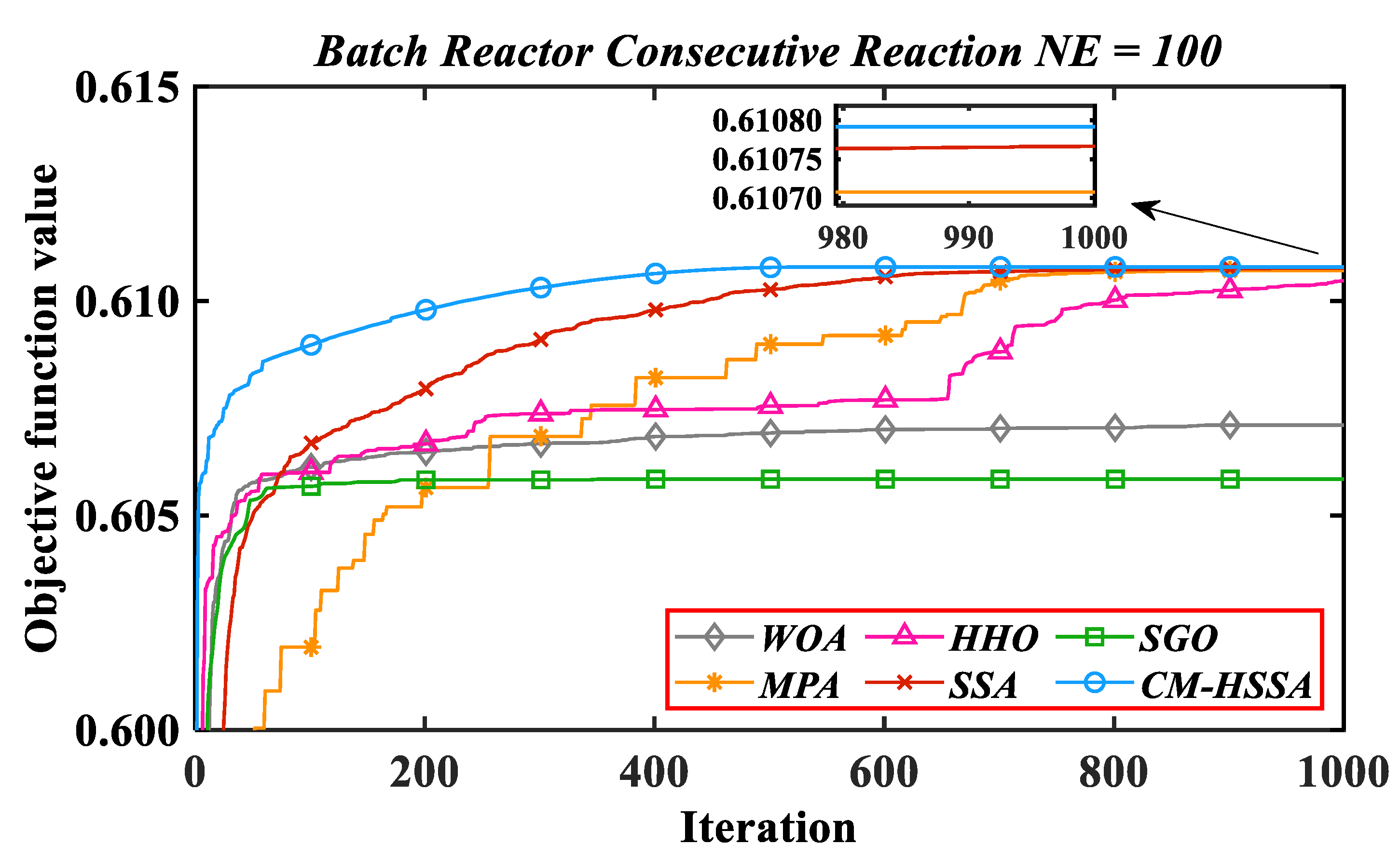
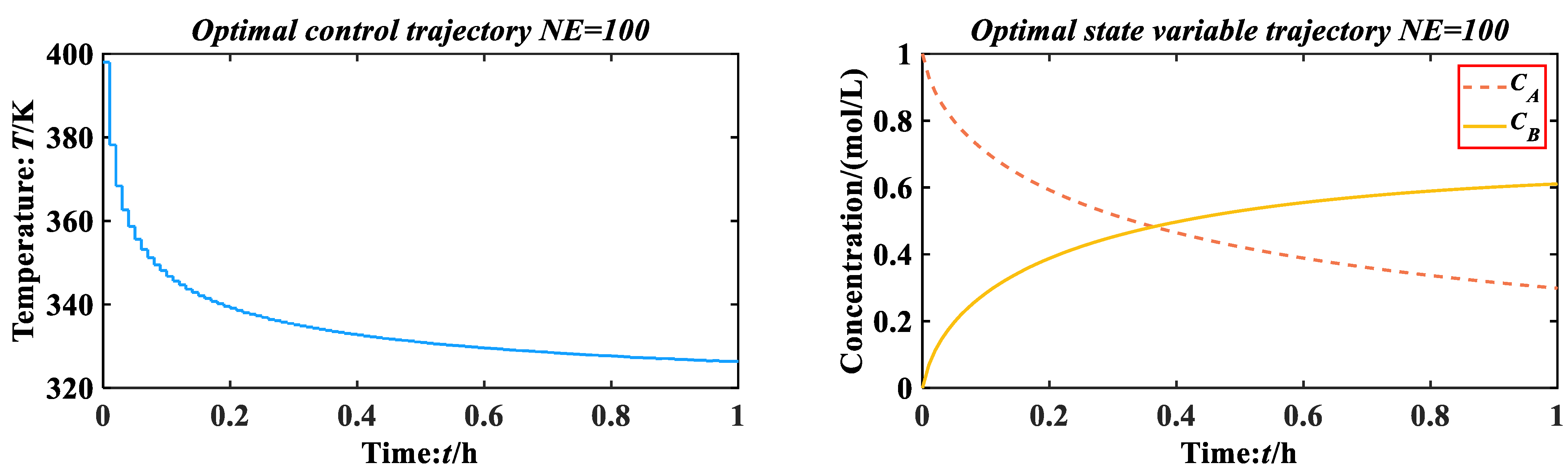
4.1. Problem 1: Batch Reactor Consecutive Reaction

The batch reactor consecutive reaction is a classic dynamic optimization problem that has been widely cited as a research object. For a batch reactor with a constructive chemical reaction, temperature control plays a key role in the formation of products. In the initial stage, it is necessary to provide a higher temperature to meet the conditions of reaction start-up. With the progress of the reaction, the temperature needs to be continuously reduced to ensure the maximum concentration of the target product. Therefore, the optimization goal of this problem is to determine an optimal temperature control trajectory to optimize the concentration of target product B generated by reactant A within 1 h of reaction. The mathematical model of batch reactor constructive reaction problem is described as follows [49]:

$$\begin{array}{c}\max J(t_f)=C_B(t_f)\\ s.t.\{\begin{array}{l}\frac{d{C}_A}{dt}=-k_1{C}_A^2\\ \frac{d{C}_B}{dt}=k_1{C}_A^2-k_2{C}_B\\ t_f=1\\ k_1=4\times {10}^3\times e^{-2500/T}\\ k_2=6.2\times {10}^5\times e^{-5000/T}\\ 298\le T\le 398, C_A(0)=1, C_B(0)=0\end{array}\end{array}$$

(17)

where $C_A$ is the reactant concentration, $C_B$ is the target product concentration, $T$ is the reaction temperature, and $t_f$ is the reaction termination time. Figure 20 shows the iterative trajectories of six algorithms to solve problem 1 when NE = 100.

Table 4. Comparison of optimization results for Problem 1.

Method	Mean	Std.	TIC/TOC
WOA	0.60718532	5.9120 × 10−4	359.5657
MPA	0.61070726	7.8608 × 10−4	344.6441
HHO	0.61047035	1.9521 × 10−3	1092.0483
SSA	0.61077333	2.4912 × 10−7	351.2811
SGO	0.60584429	9.7315 × 10−4	767.8168
CM-HSSA	0.61079200	2.9799 × 10−7	347.2429

records the mean value (mol/L), standard deviation, and mean calculation time (t/s) in 20 experiments. From the experimental results, we can see the difference between CM-HSSA and other algorithms.

By comparing the results in Table 4, CM-HSSA has the highest accuracy, and the small standard deviation shows that the result is stable. Ranking of other algorithms: SSA > MPA > HHO > WOA > SGO. In terms of calculation time, the difference between WOA, MPA, SSA, and CM-HSSA is within 15 s, while SGO and HHO are much longer. According to the literature [3], 99.95% of the highest average accuracy of the six algorithms is defined as a satisfactory solution, and their performance of the convergence rate is evaluated according to the iterations of reaching the satisfactory solution. For problem 1, the satisfactory solution is 0.6104866. WOA, HHO, and SGO failed to reach the satisfactory solution. CM-HSSA takes 346 iterations to reach the satisfactory solution, while MPA and SSA take 706 iterations and 573 iterations. That is to say, compared with MPA and SSA, iterations are reduced by 50.99% and 39.61%, respectively, with CM-HSSA. Figure 21 shows the optimal control trajectory and optimal state variable trajectory of CM-HSSA solving problem 1. To further illustrate the advantages of the obtained results, the data in different references are recorded and compared with CM-HSSA, as shown in

Table 5. Comparison of optimization results for Problem 1.

Method	NE	J/(mol/L)
OC [50]	-	0.61
SQP [51]	80	0.610775
IDP [52]	80	0.610775
PSO-CVP [12]	-	0.6105359
IKEA [53]	10	0.6101
	20	0.610426
	100	0.610781–0.610789
HIGA [54]	10	0.61007
	20	0.61046
IKBCA [17]	10	0.6101
	20	0.610454
	100	0.610779–0.610787
EBSO [13]	10	0.610558922
	20	0.61064758
	80	0.61078114
MSFO [16]	50	0.610771–0.610785
ISOA [15]	30	0.61059223
CVP-PSO [3]	-	0.6107847
CVP-APSO [3]	-	0.6107850
This work (CM-HSSA)	100	0.61079200

.

According to Table 5: Renfro et al. [50] obtained a result of 0.61 using the orthogonal collocation (OC) method, Logsdon et al. [51] obtained 0.610775 by using the SQP strategy, while the iterative dynamic programming (IDP) method used in reference [52] obtained the same result, Shi et al. [12] used PSO to solve the problem under the CVP framework and obtained 0.6105359, Peng et al. [53] obtained 0.610781 to 0.610789 by using the proposed IKEA, and the accuracy is slightly better than HIGA [54], which is generally consistent with the results of IKBCK [17]. The EBSO proposed by Lyu et al. [13] is better than the three algorithms mentioned above when the number of segments is small, but the accuracy improved by the algorithm is not obvious through the increased segments, The MSFO used by Zhang et al. [16] best obtained 0.610785. The ISOA proposed by Xu et al. [15] obtained 0.61059223 in the case of equal division of 30 segments. The results are poor compared with EBSO [13], and the accuracy is limited due to the small number of segments. In this paper, CM-HSSA is used to solve problem 1, and 0.61079200 is obtained in the case of equal division of 100 segments. By comparing the above references, it can be seen that the result obtained by CM-HSSA is the best, reaching the level of 0.61079, which is slightly better than the best value of 0.6107850 in reference [3], which shows that CM-HSSA is feasible and effective to solve the batch reactor consecutive reaction problem.

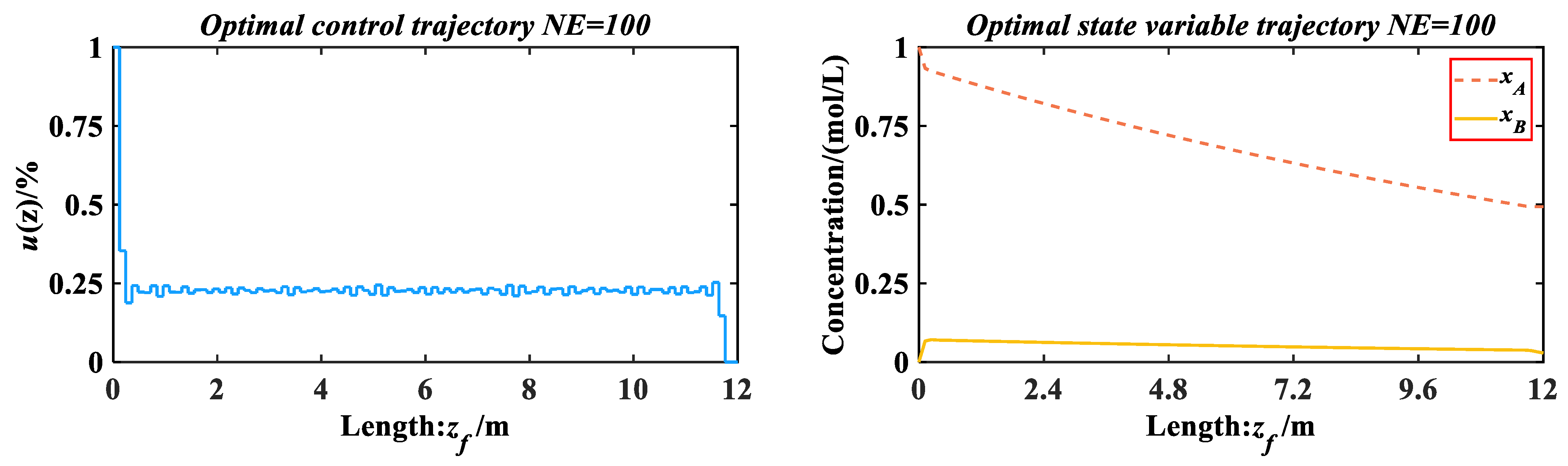
4.2. Problem 2: Catalyst Mixing Reaction in Tubular Reactor

The problem of the catalyst mixing reaction in the tubular reactor was first proposed by Gunn et al. [55] in 1965. This problem can be briefly described as: in a tubular reactor with a certain length, the two catalysts A and B are mixed to produce the target product C. Therefore, the dynamic optimization involved in this problem is to optimize the output of target product C in a fixed-length tubular reactor by regulating the catalyst concentration in the mixture. It is worth noting that the reaction process takes place in an isothermal tubular reactor by default. The mathematical model of catalyst mixing reaction in the tubular reactor is as follows:

$$\begin{array}{c}\max J(z_f)=1-x_A(z_f)-x_B(z_f)\\ s.t.\{\begin{array}{l}\frac{d{x}_A}{dz}=-u(z)[10\times x_B(z)-x_A(z)]\\ \frac{d{x}_B}{dz}=u(z)[10\times x_B(z)-x_A(z)]-[1-u(z)]\times x_B(z)\\ z_f=12\\ 0\le u(z)\le 1, x_A(0)=1, x_B(0)=0\end{array}\end{array}$$

(18)

where $x_A$ and $x_B$ are the mole fractions of A and B in the mixture, $z_f$ is the length of the tubular reactor, and $u(z)$ is the mixing fraction of catalyst A. Figure 22 shows the iterative trajectories of six algorithms to solve problem 2 when NE = 100.

Table 6. Comparison of optimization results for Problem 2.

Method	Mean	Std.	TIC/TOC
WOA	0.47625678	5.8233 × 10−4	426.7259
MPA	0.47742011	6.4257 × 10−4	1034.2457
HHO	0.47478338	1.7305 × 10−3	1213.1210
SSA	0.47744034	9.2403 × 10−4	503.7366
SGO	0.47530289	3.8821 × 10−4	1161.0388
CM-HSSA	0.47770179	2.7368 × 10−5	457.1058

records the mean value (mol/L), standard deviation, and mean calculation time (t/s) in 20 experiments.

It can be seen from the results in Table 6 that CM-HSSA has the most stable and highest solution accuracy. In terms of optimization accuracy, ranking of other algorithms is as follows: SSA > MPA > WOA > SGO > HHO. In terms of calculation time, the difference between WOA, SSA, and CM-HSSA is within 78 s, while MPA, SGO, and HHO are much longer. In terms of convergence rate, only CM-HSSA reaches a satisfactory solution and takes 103 iterations. MPA and SSA are close to the satisfactory solution of 0.47746294, but they have not achieved this value with 1000 iterations. Figure 23 shows the optimal control trajectory and optimal state variable trajectory of CM-HSSA solving problem 2. To further illustrate the advantages of the obtained results, the data in different references are recorded and compared with CM-HSSA, as shown in

Table 7. Comparison of optimization results for Problem 2.

Methods	NE	J/(mol/L)
IDP [52]	20	0.47527
	40	0.47695
ACO [14]	-	0.47615
IKEA [53]	10	0.475
	20	0.4757
	100	0.47761–0.47768
IKBCA [17]	20	0.4753
	100	0.47768–0.47770
EBSO [13]	10	0.47502183
	20	0.47627191
	40	0.47697288
MSFO [16]	20	0.47562
	70	0.477544–0.47760
ISOA [15]	40	0.47721
This work (CM-HSSA)	100	0.47770179

.

It can be seen from Table 7 that the highest accuracy of IDP [52] is 0.47695, which is slightly better than the result solved by Rajesh et al. [14] using ACO. The result obtained by MSFO [16] is 0.477544–0.47760, which is inferior to the accuracy achieved by IKEA [53] and IKBCA [17]. ISOA [15] achieved 0.47721, and its accuracy is better than that of EBSO [13] in the same segmentation. When the segment is 100, CM-HSSA obtains a result of 0.47770179 for solving the catalyst mixing reaction in a tubular reactor compared with other references; only the proposed algorithm can stably reach the level of 0.4777, while the accuracy of different methods hovers in the range of 0.475–0.476. Therefore, CM-HSSA has a better solution effect than other methods, which further proves the effectiveness of the algorithm proposed in this paper.

4.3. Problem 3: Parallel Reactions in Tubular Reactor

The parallel reaction problem in the tubular reactor is a dynamic optimization problem with saturation characteristics of control variables [56], and it has been cited by many researchers. In the tubular reactor, there is a side reaction process ($A\to C$) parallel to the main reaction ($A\to B$), so the optimization goal of this problem is to maximize the target product B of the main reaction at the end by determining an optimal control trajectory. Similarly, all reactions of this problem occur in an isothermal tubular reactor by default. The mathematical model of parallel reactions in the tubular reactor is as follows:

$$\begin{array}{c}\max J(t_f)=x_B(t_f)\\ s.t.\{\begin{array}{l}\frac{d{x}_A}{dt}=-[u(t)+0.5u^2(t)]x_A(t)\\ \frac{d{x}_B}{dt}=u(t)x_A(t)\\ t_f=1\\ 0\le u(t)\le 5, x_A(0)=1, x_B(0)=0\end{array}\end{array}$$

(19)

where $x_A$ is the concentration of reactant A, $x_B$ is the concentration of target product B, $t_f$ is the reaction termination time, and $u(t)$ is the saturation of the control variable. Figure 24 shows the iterative trajectories of six algorithms to solve problem 3 when NE = 100.

Table 8. Comparison of optimization results for Problem 3.

Method	Mean	Std.	TIC/TOC
WOA	0.56836465	1.4475 × 10−3	364.3671
MPA	0.57349880	1.0338 × 10−3	381.3942
HHO	0.57152795	2.9227 × 10−3	1062.2493
SSA	0.57269740	8.7921 × 10−3	349.0882
SGO	0.55138595	3.5277 × 10−4	685.3328
CM-HSSA	0.57355371	4.2218 × 10−6	376.5377

records the mean value (mol/L), standard deviation, and mean calculation time (t/s) in 20 experiments.

By comparing the results in Table 8, CM-HSSA also obtains the highest accuracy and the smallest standard deviation among the six algorithms, and the ranking of other algorithms is as follows: MPA > SSA > HHO > WOA > SGO. In terms of calculation time, except for SGO and HHO, the difference between the other four algorithms is within 33 s. In terms of convergence rate, CM-HSSA takes only 98 iterations to achieve a satisfactory solution of 0.57326693, while MPA takes 671 iterations, so the iterations are reduced by 85.39% with CM-HSSA. Other algorithms failed to reach this value. Through comprehensive comparison, CM-HSSA has more advantages and wider applicability in optimization performance and calculation efficiency. Figure 25 shows the optimal control trajectory and optimal state variable trajectory of CM-HSSA solving problem 3. To further confirm the superiority of the results obtained, the data in different references are recorded and compared with CM-HSSA, as shown in

Table 9. Comparison of optimization results for Problem 3.

Methods	NE	J/(mol/L)
IDP [52]	20	0.57330
	40	0.57348
	80	0.57353
CVP [57]	-	0.56910
CVI [57]	-	0.57322
ACO [14]	-	0.57284
CP-PSO [3]	-	0.573543
CP-APSO [3]	-	0.573544
ISOA [15]	40	0.573073
This work (CM-HSSA)	100	0.57355371

.

According to Table 9, the IDP [52] divided into 80 segments has the best result of 0.57353. Biegler [57] proposed combining successive quadratic programming and orthogonal collocation, and obtained 0.56910 and 0.57322 based on CVP and control vector iteration (CVI), respectively. ACO [14] solved the problem and obtained 0.57284, which is lower than other methods. Zhou et al. [3] proposed a dynamic optimization control parameter solution and obtained 0.573544 using APSO, which is improved compared with PSO. Xu et al. [15] divided it into 40 segments and obtained the best result of 0.573073. Compared with these references, the solution of CM-HSSA has reached the highest accuracy level of the current optimization for this problem, and is slightly better than the result of 0.573544 obtained in reference [3], which further verifies the ability of CM-HSSA to solve dynamic optimization problems.

5. Conclusions

This manuscript introduced a novel SSA algorithm named CM-HSSA that further enhanced both the exploration and exploitation abilities of the original method. Through the benchmark function experiments, compared with WOA, MPA, HHO, SSA, and SGO, the statistical results verify that CM-HSSA has more advantages in stability, accuracy, and convergence rate. Under a universal swarm-intelligence dynamic optimization framework, the above six algorithms are used to solve three typical chemical dynamic optimization problems, and the simulation results further validate the applicability of CM-HSSA to solve the dynamic optimization problems. Compared with different methods in the literature, CM-HSSA also achieved the best results.

For dynamic optimization problems, in addition to the performance of the optimization algorithm affecting the final results, the segmentation of the time domain and the selection of the approximation method for control variables will also have different effects on the solution. In future work, we will conduct more research on these two aspects, and use high-performance optimization algorithms to solve complex dynamic optimization problems with strong nonlinearity.

References

1. Zhang, B.; Chen, D.; Wu, X. Graded optimization strategy and its application to chemical dynamic optimization with fixed boundary. CIESC J. 2005, 56, 1276–1280. [Google Scholar]
2. Mo, Y.; Chen, D. Chaos particle swarm optimization algorithm and its application in biochemical process dynamic optimization. CIESC J. 2006, 57, 2123–2127. [Google Scholar]
3. Zhou, Y.; Liu, X. Control parameterization-based adaptive particle swarm approach for solving chemical dynamic optimization problems. Chem. Eng. Technol. 2014, 37, 692–702. [Google Scholar] [CrossRef]
4. Sun, Y.; Zhang, M.; Liang, X. Improved Gauss pseudospectral method for solving a nonlinear optimal control problem with complex constraints. Acta Autom. Sin. 2013, 39, 672–678. [Google Scholar] [CrossRef]
5. Chachuat, B.; Mitsos, A.; Barton, P.I. Optimal design and steady-state operation of micro power generation employing fuel cells. Chem. Eng. Sci. 2005, 60, 4535–4556. [Google Scholar] [CrossRef]
6. Peng, H.; Gao, Q.; Wu, Z.; Zhong, W. A mixed variable variational method for optimal control problems with applications in aerospace control. Acta Autom. Sin. 2011, 37, 1248–1255. [Google Scholar]
7. Pollard, G.P.; Sargent, R.W.H. Off line computation of optimum controls for a plate distillation column. Automatica 1970, 6, 59–76. [Google Scholar] [CrossRef]
8. Schranz, M.; Di Caro, G.A.; Schmickl, T.; Elmenreich, W. Swarm intelligence and cyber-physical systems: Concepts, challenges and future trends. Swarm Evol. Comput. 2021, 60, 100762. [Google Scholar] [CrossRef]
9. Hussain, K.; Mohd, M.N.; Cheng, S. Metaheuristic research: A comprehensive survey. Artif. Intell. Rev. 2019, 52, 2191–2233. [Google Scholar] [CrossRef] [Green Version]
10. Bacanin, N.; Stoean, R.; Zivkovic, M.; Petrovic, A.; Rashid, T.A.; Bezdan, T. Performance of a novel chaotic firefly algorithm with enhanced exploration for tackling global optimization problems: Application for dropout regularization. Mathematics 2021, 9, 2705. [Google Scholar] [CrossRef]
11. Malakar, S.; Ghosh, M.; Bhowmik, S.; Sarkar, R.; Nasipuri, M. A GA based hierarchical feature selection approach for handwritten word recognition. Neural Comput. Appl. 2020, 32, 2533–2552. [Google Scholar] [CrossRef]
12. Shi, B.; Yin, Y.; Liu, F. Optimal control strategies combined with PSO and control vector parameterization for batchwise chemical process. CIESC J. 2019, 70, 979–986. [Google Scholar]
13. Lyu, Y.; Mo, Y.; Lu, Y.; Liu, R. Enhanced Beetle Antennae Algorithm for Chemical Dynamic Optimization Problems’ Non-Fixed Points Discrete Solution. Processes 2022, 10, 148. [Google Scholar] [CrossRef]
14. Asgari, S.A.; Pishvaie, M.R. Dynamic Optimization in Chemical Processes Using Region Reduction Strategy and Control Vector Parameterization with an Ant Colony Optimization Algorithm. Chem. Eng. Technol. Ind. Chem. Plant Equip. Process. Eng. Biotechnol. 2008, 31, 507–512. [Google Scholar] [CrossRef]
15. Xu, L.; Mo, Y.; Lu, Y. Improved Seagull Optimization Algorithm Combined with an Unequal Division Method to Solve Dynamic Optimization Problems. Processes 2021, 9, 1037. [Google Scholar] [CrossRef]
16. Zhang, Y.; Mo, Y. Dynamic optimization of chemical processes based on modified sailfish optimizer combined with an equal division method. Processes 2021, 9, 1806. [Google Scholar] [CrossRef]
17. Liu, Z.; Du, W.L.; Qi, R. Dynamic optimization in chemical processes using improved knowledge-based cultural algorithm. CIESC J. 2010, 61, 2889–2895. [Google Scholar]
18. Mirjalili, S.; Lewis, A. The whale optimization algorithm. Adv. Eng. Softw. 2016, 95, 51–67. [Google Scholar] [CrossRef]
19. Faramarzi, A.; Heidarinejad, M.; Mirjalili, S. Marine Predators Algorithm: A nature-inspired metaheuristic. Expert Syst. Appl. 2020, 152, 113377. [Google Scholar] [CrossRef]
20. Heidari, A.A.; Mirjalili, S.; Faris, H. Harris hawks optimization: Algorithm and applications. Future Gener. Comput. Syst. 2019, 97, 849–872. [Google Scholar] [CrossRef]
21. Satapathy, S.; Naik, A. Social group optimization (SGO): A new population evolutionary optimization technique. Complex Intell. Syst. 2016, 2, 173–203. [Google Scholar] [CrossRef] [Green Version]
22. Fathy, A.; Alanazi, T.M.; Rezk, H.; Yousri, D. Optimal energy management of micro-grid using sparrow search algorithm. Energy Rep. 2022, 8, 758–773. [Google Scholar] [CrossRef]
23. Zhang, Z.; Han, Y. Discrete sparrow search algorithm for symmetric traveling salesman problem. Appl. Soft Comput. 2022, 118, 108469. [Google Scholar] [CrossRef]
24. Yan, S.; Yang, P.; Zhu, D. Improved Sparrow Search Algorithm Based on Iterative Local Search. Comput. Intell. Neurosci. 2021, 2021, 6860503. [Google Scholar] [CrossRef]
25. Xiong, Q.; Zhang, X.; He, S. A Fractional-Order Chaotic Sparrow Search Algorithm for Enhancement of Long Distance Iris Image. Mathematics 2021, 9, 2790. [Google Scholar] [CrossRef]
26. Zhang, C.; Ding, S. A stochastic configuration network based on chaotic sparrow search algorithm. Knowl. Based Syst. 2021, 220, 106924. [Google Scholar] [CrossRef]
27. Mirjalili, S.; Mirjalili, S.M.; Lewis, A. Grey wolf optimizer. Adv. Eng. Softw. 2014, 69, 46–61. [Google Scholar] [CrossRef] [Green Version]
28. Rashedi, E.; Nezamabadi-Pour, H.; Saryazdi, S. GSA: A gravitational search algorithm. Inf. Sci. 2009, 179, 2232–2248. [Google Scholar] [CrossRef]
29. Mirjalili, S. SCA: A sine cosine algorithm for solving optimization problems. Knowl. Based Syst. 2016, 96, 120–133. [Google Scholar] [CrossRef]
30. Liu, G.; Shu, C.; Liang, Z. A modified sparrow search algorithm with application in 3d route planning for UAV. Sensors 2021, 21, 1224. [Google Scholar] [CrossRef]
31. Ma, J.; Hao, Z.; Sun, W. Enhancing sparrow search algorithm via multi-strategies for continuous optimization problems. Inf. Process. Manag. 2022, 59, 102854. [Google Scholar] [CrossRef]
32. Shi, L.; Ding, X.; Li, M. Research on the capability maturity evaluation of intelligent manufacturing based on firefly algorithm, sparrow search algorithm, and BP neural network. Complexity 2021, 2021, 5554215. [Google Scholar] [CrossRef]
33. Ouyang, C.; Qiu, Y.; Zhu, D. Adaptive spiral flying sparrow search algorithm. Sci. Program. 2021, 2021, 6505253. [Google Scholar] [CrossRef]
34. Nguyen, T.T.; Ngo, T.G.; Dao, T.K. Microgrid Operations Planning Based on Improving the Flying Sparrow Search Algorithm. Symmetry 2022, 14, 168. [Google Scholar] [CrossRef]
35. Chen, X.; Tianfield, H.; Mei, C. Biogeography-based learning particle swarm optimization. Soft Comput. 2017, 21, 7519–7541. [Google Scholar] [CrossRef]
36. Luyben, W.L. Optimum product recovery in chemical process design. Ind. Eng. Chem. Res. 2014, 53, 16044–16050. [Google Scholar] [CrossRef]
37. Tavazoei, M.S.; Haeri, M. Comparison of different one-dimensional maps as chaotic search pattern in chaos optimization algorithms. Appl. Math. Comput. 2007, 187, 1076–1085. [Google Scholar] [CrossRef]
38. Li, Y.; Han, M.; Guo, Q. Modified whale optimization algorithm based on tent chaotic mapping and its application in structural optimization. KSCE J. Civ. Eng. 2020, 24, 3703–3713. [Google Scholar] [CrossRef]
39. Varol Altay, E.; Alatas, B. Bird swarm algorithms with chaotic mapping. Artif. Intell. Rev. 2020, 53, 1373–1414. [Google Scholar] [CrossRef]
40. Han, X.H.; Xiong, X.; Duan, F. A new method for image segmentation based on BP neural network and gravitational search algorithm enhanced by cat chaotic mapping. Appl. Intell. 2015, 43, 855–873. [Google Scholar] [CrossRef]
41. Sayed, G.I.; Tharwat, A.; Hassanien, A.E. Chaotic dragonfly algorithm: An improved metaheuristic algorithm for feature selection. Appl. Intell. 2019, 49, 188–205. [Google Scholar] [CrossRef]
42. Koyuncu, H. GM-CPSO: A new viewpoint to chaotic particle swarm optimization via Gauss map. Neural Process. Lett. 2020, 52, 241–266. [Google Scholar] [CrossRef]
43. Yuan, J.; Liu, Z.; Lian, Y. Global Optimization of UAV Area Coverage Path Planning Based on Good Point Set and Genetic Algorithm. Aerospace 2022, 9, 86. [Google Scholar] [CrossRef]
44. Tang, Y.; Wang, Z.; Fang, J. Feedback learning particle swarm optimization. Appl. Soft Comput. 2011, 11, 4713–4725. [Google Scholar] [CrossRef] [Green Version]
45. Brockmann, D.; Hufnagel, L.; Geisel, T. The scaling laws of human travel. Nature 2006, 439, 462–465. [Google Scholar] [CrossRef]
46. Mantegna, R.N. Fast, accurate algorithm for numerical simulation of Levy stable stochastic processes. Phys. Rev. E 1994, 49, 4677. [Google Scholar] [CrossRef]
47. Mirjalili, S. Dragonfly algorithm: A new meta-heuristic optimization technique for solving single-objective, discrete, and multi-objective problems. Neural Comput. Appl. 2016, 27, 1053–1073. [Google Scholar] [CrossRef]
48. Derrac, J.; García, S.; Molina, D. A practical tutorial on the use of nonparametric statistical tests as a methodology for comparing evolutionary and swarm intelligence algorithms. Swarm Evol. Comput. 2011, 1, 3–18. [Google Scholar] [CrossRef]
49. Rajesh, J.; Gupta, K.; Kusumakar, H.S. Dynamic optimization of chemical processes using ant colony framework. Comput. Chem. 2001, 25, 583–595. [Google Scholar] [CrossRef]
50. Renfro, J.G.; Morshedi, A.M.; Asbjornsen, O.A. Simultaneous optimization and solution of systems described by differential/algebraic equations. Comput. Chem. Eng. 1987, 11, 503–517. [Google Scholar] [CrossRef]
51. Logsdon, J.S.; Biegler, L.T. A relaxed reduced space SQP strategy for dynamic optimization problems. Comput. Chem. Eng. 1993, 17, 367–372. [Google Scholar] [CrossRef]
52. Dadebo, S.A.; McAuley, K.B. Dynamic optimization of constrained chemical engineering problems using dynamic programming. Comput. Chem. Eng. 1995, 19, 513–525. [Google Scholar] [CrossRef]
53. Peng, X.; Qi, R.; Du, W.; Qian, F. An improved knowledge evolution algorithm and its application to chemical process dynamic optimization. CIESC J. 2012, 63, 841–850. [Google Scholar]
54. Sun, F.; Du, W.; Qi, R. A hybrid improved genetic algorithm and its application in dynamic optimization problems of chemical processes. Chin. J. Chem. Eng. 2013, 21, 144–154. [Google Scholar] [CrossRef]
55. Gunn, D.J.; Thomas, W.J. Mass transport and chemical reaction in multifunctional catalyst systems. Chem. Eng. Sci. 1965, 20, 89–100. [Google Scholar] [CrossRef]
56. Liu, X.; Chen, L.; Hu, Y. Solution of chemical dynamic optimization using the simultaneous strategies. Chin. J. Chem. Eng. 2013, 21, 55–63. [Google Scholar] [CrossRef]
57. Biegler, L.T. Solution of dynamic optimization problems by successive quadratic programming and orthogonal collocation. Comput. Chem. Eng. 1984, 8, 243–247. [Google Scholar] [CrossRef]
Figure 1. Piecewise constant approximation of CVP method.
Mathematics 10 01803 g001
Figure 2. Swarm-Intelligence Dynamic Optimization Method Based on CVP Strategy.
Mathematics 10 01803 g002
Figure 3. The flowchart of SSA.
Mathematics 10 01803 g003
Figure 4. Comparison of two different initialization strategies.
Mathematics 10 01803 g004
Figure 5. Average value distributions of seven different initialization strategies.
Mathematics 10 01803 g005
Figure 6. Producers’ location update trends ( R 2 < S T ).
Mathematics 10 01803 g006
Figure 7. The changing trend of the inertia weight factor.
Mathematics 10 01803 g007
Figure 8. Lévy flight and Brownian motion.
Mathematics 10 01803 g008
Figure 9. Boxplot of six algorithms for benchmark functions.
Mathematics 10 01803 g009
Figure 10. Sphere Model.
Mathematics 10 01803 g010
Figure 11. Schwefel’s problem 2.22.
Mathematics 10 01803 g011
Figure 12. Schwefel’s problem 1.2.
Mathematics 10 01803 g012
Figure 13. Schwefel’s problem 2.21.
Mathematics 10 01803 g013
Figure 14. Generalized Schwefel’s problem 2.26.
Mathematics 10 01803 g014
Figure 15. Generalized Rastrigin’s Function.
Mathematics 10 01803 g015
Figure 16. Ackley’s Function.
Mathematics 10 01803 g016
Figure 17. Generalized Griewank Function.
Mathematics 10 01803 g017
Figure 18. Branin Function.
Mathematics 10 01803 g018
Figure 19. Goldstein−Price Function.
Mathematics 10 01803 g019
Figure 20. Iterative trajectories of six algorithms for Problem 1.
Mathematics 10 01803 g020
Figure 21. CM-HSSA for Problem 1.
Mathematics 10 01803 g021
Figure 22. Iterative trajectories of six algorithms for Problem 2.
Mathematics 10 01803 g022
Figure 23. CM-HSSA for Problem 2.
Mathematics 10 01803 g023
Figure 24. Iterative trajectories of six algorithms for Problem 3.
Mathematics 10 01803 g024
Figure 25. CM-HSSA for Problem 3.
Mathematics 10 01803 g025