Article

Topology Identification of Time-Scales Complex Networks

1
College of Computer Science and Technology, Nanjing University of Aeronautics and Astronautics, Nanjing 210016, China
2
School of Intelligent Engineering, Jiangsu Vocational Institute of Commerce, Nanjing 211168, China
3
School of Mathematics and Systems Science, Guangdong Polytechnic Normal University, Guangzhou 510665, China
4
Department of Mathematics, Center for Dynamics, Technische Universität, 01069 Dresden, Germany
*
Author to whom correspondence should be addressed.
Mathematics 2022, 10(10), 1755; https://doi.org/10.3390/math10101755
Submission received: 21 April 2022 / Revised: 16 May 2022 / Accepted: 17 May 2022 / Published: 21 May 2022
(This article belongs to the Topic Complex Systems and Network Science)

Abstract

:
This paper studies a topology identification problem of complex networks with dynamics on different time scales. Using the adaptive synchronization method, some criteria for a successful estimation are obtained. In particular, by regulating the original network to synchronize with an auxiliary chaotic network, this work further explores a way to avoid the precondition of linear independence. When the adaptive controller fails to achieve the outer synchronization, an impulsive control method is used. In the end, we conclude with three numerical simulations. The results obtained in this paper generalize continuous, discrete with arbitrary time step size and mixed cases.

1. Introduction

Complex networks are becoming increasingly popular in the study of networked dynamic systems, including disease transmission networks, metabolic networks, social networks, communication networks, the Internet, and so on [1]. In these networks, topology structure describes the coupling states between nodes and plays a key role in the generation of collective dynamic behaviors [2,3,4]. However, in reality, many network topologies are sometimes unknown or uncertain. For instance, if a malfunction occurs in a communication network, power grid, or the Internet, it is very important to locate the faulty position [5]. As a result, network topology identification is worth investigating.
In the past decade, many methods have been studied for topology identification, such as the chaotic ant swarm algorithm [6], ROC curve analysis [7], and outer synchronization [8]. Among them, the synchronization-based topology identification method [5,8,9,10,11,12,13] has gained a lot of attention. In brief, this method first takes the unknown topology network as the driver network, and then constructs an auxiliary network with a coupling estimator and adaptive controllers as the response network. The topology is inferred by the coupling estimator when outer synchronization is achieved between the drive network and the response network. The synchronization-based method has been employed to investigate various network models, such as delayed networks, fractional networks, and multi-layer networks, see [14,15,16,17,18]. In [19,20,21,22,23], different forms of outer synchronization have been considered for topology identification, for example, adaptive lag synchronization, anticipatory synchronization, and generalized outer synchronization. In [24,25,26], several control methods have been exploited for network synchronization. It is worth mentioning that most references were considered under an assumption of linear independence of inner coupling function, which means the identification would fail if the partial or full inner synchronization occurs on the network, see [27]. This motivates some researchers to deal with this problem. In [18], Zhao et al. added sinusoidal interference signals to the original network to destroy the inner synchronization. In [28], Zhu et al. added a regulation mechanism to the network to be identified and constructed an auxiliary network consisting of isolated nodes of periodic nonlinear dynamical behavior. In [29], Liu et al. regulated the original network to synchronize with an auxiliary network composed of isolated chaotic systems to avoid the inner synchronization.
It should be noted that most existing relevant literature on the structure identification of complex dynamical networks is considered for continuous systems. Given that in the real world, the dynamics of networks are not only continuous, but also discrete, and sometimes even hybrid. For instance, a computer control system is a discrete system. Furthermore, the signal transmission in such networks is not continuous, but intermittent. With this motivation, the theory of time scale, which unifies continuous and discrete cases into one theoretical framework, provides a new idea for the study of this problem. Recently, this novel mathematical theory has been applied to various researches [30,31,32,33,34,35], especially in the synchronization of complex networks. Some general results about synchronization conclusions [16,32,36] and control criteria [35,37,38] have been generated.
Inspired by the identification works in [5,8,9,27,39], and the improved methods in [28,29], we investigate the topology identification of complex networks with different time scales in this paper. The main contributions are summarized as follows:
  • We discuss the topology identification of complex networks on the theory of time scales, which makes the proposed criteria more general. These criteria not only applies to the continuous cases, but also to the discrete cases with arbitrary time step, and even to the intermittent cases;
  • To overcome the identification failure caused by the inner synchronization of complex network, we improve the synchronization-based method on time scales by constructing a chaotic auxiliary network;
  • An impulsive control method is developed ensuring that the outer synchronization is between the original network and the auxiliary network. Impulsive control criteria are offered on time scales.
The paper is organized as follows. We begin by recalling some preliminaries in Section 2. The topology identification of complex dynamical networks is discussed in Section 3. A new topology identification model and an impulsive control method are proposed in Section 4. In Section 5, numerical simulations are performed.

2. Preliminaries

In this section, some basics on time scales and notations are introduced. For a monograph on time scales, we recommend the interested reader to [40].
Let R , Z and N be the set of the real numbers, integers, and natural numbers, respectively. A time scale T is an arbitrary non-empty closed subset of R . Denote h Z : = h k : h N , k Z . N + : = N { 0 } . μ : T 0 , is a graininess function which is defined by
μ ( t ) : = σ ( t ) t ,
where σ ( t ) : = inf { r T : r > t } is the forward jump operator. t is right-dense if σ ( t ) = t and right-scattered if σ ( t ) > t . · denotes the usual Euclidean norm. ⊗ is the Kronecker product which is defined by
A B = a 11 B a 12 B a 1 q B a 21 B a 22 B a 2 q B a p 1 B a p 2 B a p q B
for a matrix A = ( a i j ) R p × q and any matrix B. I q stands for a q × q identity matrix.
Definition 1
([40]). A function p : T R is regressive provided
1 + μ ( t ) p ( t ) 0 for all t T .
The set of all regressive functions is denoted by R .
Definition 2
([40]). We define the set R + : = of all positively regressive elements of R by
R + R + ( T , R ) = { p R : 1 + μ ( t ) p ( t ) > 0 for all t T } .
Definition 3
([40]). Let p , q R + . We define the time scale circle plus by
( p q ) ( t ) : = p ( t ) + q ( t ) + μ ( t ) p ( t ) q ( t ) for all t T .
Definition 4
([40]). Let x : T R m . Then, the time scale derivative x Δ is defined by
x Δ ( t ) = lim r t , r T x ( t ) x ( r ) t r if t is right - dense , x ( σ ( t ) ) x ( t ) μ ( t ) if t is right - scattered .
Definition 5
([40]). Let f : T R . We define the Cauchy integral by
s r f ( t ) Δ t = F ( s ) F ( r ) for all r , s T ,
where F Δ ( t ) = f ( t ) for all t [ r , s ] .
Lemma 1
([40]). Assume functions ψ , ω : T R m , ψ and ω are differentiable at t T . Then, the following identities hold:
ψ ( σ ( t ) ) = ψ ( t ) + μ ( t ) ψ Δ ( t ) ,
( ψ ω ) Δ ( t ) = ψ Δ ( t ) ω ( t ) + ψ ( t ) ω Δ ( t ) + μ ( t ) ψ Δ ( t ) ω Δ ( t ) .
Definition 6
([40]). If p R and t , s T , then the only solution of the initial value problem
y Δ = p ( t ) y , y ( s ) = 1
is called the time scales exponential function and denoted by e p ( t , s ) .
Lemma 2
([40]). If p R + , then
y Δ p ( t ) y for all t T
implies
y ( t ) y ( t 0 ) e p ( t , t 0 ) for all t T .
Lemma 3
([41]). If p R + , then
e p ( t , s ) exp s t p ( τ ) Δ τ for all t > s .
Lemma 4
([42]). The linear matrix inequality (LMI)
Q ( x ) S ( x ) S T ( x ) R ( x ) > 0
is equivalent to
Q ( x ) > 0 and R ( x ) S T ( x ) Q 1 ( x ) S ( x ) > 0 ,
where Q ( x ) = Q T ( x ) and R ( x ) = R T ( x ) .

3. A Complex Network Model and Its Topology Identification

Consider a general time scale dynamical complex network of N dynamical nodes, each of which is an m-dimensional dynamical system on time scale T . The network is characterized by
x i Δ ( t ) = f ( x i ( t ) ) + j = 1 N c i j h ( x j ( t ) ) , i = 1 , 2 , , N ,
where t T , x i : T R m , x i = ( x i 1 , , x i m ) T is the state vector of the i-th node, f : R m R m is a nonlinear vector function representing the node dynamics, h : R m R m is the inner coupling function. The outer coupling matrix C = ( c i j ) R N × N is defined as c i i = j = 1 , j i N c i j . Here, c i j = c j i > 0 ( i j ) if there is a connection between node i and j. Otherwise, c i j = c j i = 0 ( i j ) . One can easily see that the topology identification of (2) is dominated by matrix C.
We assume that the state vector x i is observable and can be fully measured. Function f and h are determined. To recover the unknown matrix C, one can take (2) as the drive network and construct a time scale response network as
y i Δ ( t ) = f ( y i ( t ) ) + j = 1 N d i j ( t ) h ( y j ( t ) ) + μ i ( t ) , μ i ( t ) = k i ( t ) y i ( t ) x i ( t ) , d i j Δ ( t ) = y i ( t ) x i ( t ) T h ( x j ( t ) ) ,
where i , j = 1 , 2 , , N , t T , y i : T R m , y i = ( y i 1 , , y i m ) T is the state vector of the i-th node. The outer coupling matrix D ( t ) = ( d i j ( t ) ) R N × N is the estimation of the matrix C at time t T , d i i = j = 1 , j i N d i j , d i j = d j i ( i j ) . μ i ( t ) is the i-th adaptive controller. k i ( t ) is a positive bounded function.
Let e i ( t ) y i ( t ) x i ( t ) . We have the error dynamical network
e i Δ ( t ) = f ( y i ( t ) ) f ( x i ( t ) ) + j = 1 N d i j ( t ) h ( y j ( t ) ) c i j h ( x j ( t ) ) k i ( t ) e i ( t ) , i = 1 , 2 , , N .
Assumption 1.
Assume that there exist positive constants α and β satisfying
f ( x ) f ( y ) α x y , h ( x ) h ( y ) β x y ,
for any x , y R m .
Definition 7.
The error dynamical network (4) achieves asymptotic stability at zero solution if
e i ( t ) 0 as t , i = 1 , , N , t T .
Definition 8.
The topology of network (2) can be identified if
lim t d i j ( t ) c i j = 0 , i , j = 1 , 2 , , N , t T .
Lemma 5.
If the error dynamical network (4) achieves asymptotic stability at zero solution and the vectors h ( x j ) , j = 1 , 2 , , N , are linearly independent at the zero solution, then the topology of network (2) can be identified.
Proof. 
If lim t e i ( t ) = 0 , then from (4), we have
lim t j = 1 N d i j ( t ) h ( y j ( t ) ) c i j h ( x j ( t ) ) = lim t j = 1 N d i j ( t ) c i j h ( x j ( t ) ) = 0 .
Since h ( x j ) are linearly independent, d i j ( t ) converges to c i j as t , concluding the proof. □
Theorem 1.
Let K ( t ) = diag ( k 1 ( t ) , k 2 ( t ) , , k N ( t ) ) . Assume there exist constant ζ > 0 and θ R + : T R such that the matrix ( 2 I N μ K ) K + ζ ( α 2 + β 2 ) θ I N is invertible and
t 0 t θ ( τ ) Δ τ as t .
For all t T , if we have
Ω = ( 2 I N μ K ) K + ζ ( α 2 + β 2 ) θ I N I N μ K ( I N μ K ) D ( I N μ K ) ( D C ) I N μ K ( μ ζ ) I N μ D μ ( D C ) D ( I N μ K ) μ D μ D T D ζ I N μ D T ( D C ) ( D C ) ( I N μ K ) μ ( D C ) μ ( D C ) T D μ ( D C ) T ( D C ) 0 ,
then the error dynamical network (4) achieve asymptotical stability at zero solution.
Proof. 
Set V ( t ) : = i = 1 N e i T ( t ) e i ( t ) , t T . We have
V Δ = i = 1 N e i T Δ e i + e i T σ e i Δ = 2 i = 1 N e i T ( f ( y i ) f ( x i ) ) + 2 i = 1 N e i T j = 1 N d i j h ( y j ) h ( x j ) + 2 i = 1 N e i T j = 1 N ( d i j c i j ) h ( x j ) 2 i = 1 N k i ( y i x i ) T ( y i x i ) + μ i = 1 N ( f ( y i ) f ( x i ) ) T ( f ( y i ) f ( x i ) ) + 2 i = 1 N ( f ( y i ) f ( x i ) ) T j = 1 N d i j h ( y j ) h ( x j ) + 2 i = 1 N ( f ( y i ) f ( x i ) ) T j = 1 N d i j c i j h ( x j ) 2 i = 1 N k i ( f ( y i ) f ( x i ) ) T ( y i x i ) + i = 1 N j = 1 N d i j h ( y j ) h ( x j ) T j = 1 N d i j h ( y j ) h ( x j ) + 2 i = 1 N j = 1 N d i j ( t ) h ( y j ( t ) ) h ( x j ( t ) ) T j = 1 N d i j ( t ) c i j h ( x j ( t ) ) + i = 1 N j = 1 N d i j c i j h T ( x j ) j = 1 N d i j c i j h ( x j ) 2 i = 1 N k i j = 1 N d i j c i j h T ( x j ) ( y i x i ) 2 i = 1 N k i j = 1 N d i j h ( y j ) h ( x j ) T ( y i x i ) + i = 1 N k i 2 ( y i x i ) T ( y i x i ) , t T .
We introduce the notations
E ( t ) = ( e 1 T ( t ) , e 2 T ( t ) , , e N T ( t ) ) T , t T , G 1 ( t ) = ( g 11 T ( t ) , g 12 T ( t ) , , g 1 N T ( t ) ) T , t T , G 2 ( t ) = ( g 21 T ( t ) , g 22 T ( t ) , , g 2 N T ( t ) ) T , t T , H ( X ( t ) ) = ( h T ( x 1 ( t ) ) , h T ( x 2 ( t ) ) , , h T ( x N ( t ) ) ) T , t T ,
where g 1 i ( t ) : = f ( y i ( t ) ) f ( x i ( t ) ) , t T and g 2 i ( t ) : = h ( y i ( t ) ) h ( x i ( t ) ) , t T , i = 1 , 2 , , N .
From Assumption 1, we have
ζ G 1 T G 1 + G 2 T G 2 = ζ i = 1 N g 1 i T g 1 i + i = 1 N g 2 i T g 2 i ζ α 2 + β 2 E T E , t T .
Then, we have
V Δ θ V 2 E T G 1 + 2 E T ( D I m ) G 2 + 2 E T ( ( D C ) I m ) H ( X ) 2 E T ( ( K θ I N ) I m ) E + ζ α 2 + β 2 E T E ζ G 1 T G 1 + G 2 T G 2 + μ G 1 T G 1 + 2 G 1 T D I m G 2 + 2 G 1 T ( D C ) I m H ( X ) 2 G 1 T K I m E + G 2 T D T D I m G 2 + 2 G 2 T D T ( D C ) I m H ( X ) 2 E T K D I m G 2 + H T ( X ) ( D C ) T ( D C ) I m H ( X ) 2 E T K ( D C ) I m H ( X ) + E T K 2 I m E Q T Ω I m Q , t T ,
where Q = E T , G 1 T , G 2 T , H T ( X ) T . By (6), V Δ θ V Q T Ω I m Q 0 , i.e.,
V Δ θ V , t T .
Since θ R + , using Lemma 2, we have
0 V ( t ) e θ ( t , t 0 ) V ( t 0 ) , t T ,
where t > t 0 . Without loss of generality, we assume the initial value V ( t 0 ) 0 . According to Lemma 3, it follows that
0 e θ ( t , t 0 ) exp t 0 t θ ( τ ) Δ τ , t T .
From (5) and (11), we have e θ ( t , t 0 ) 0 as t . This leads to V ( t ) 0 as t . Since the non-negativity of V ( t ) , we have e i 0 as t . Thus, we conclude that the error systems (4) achieve asymptotic stability at their zero solution. □
Remark 1.
If the condition (6) holds, due to Lemma 4, we have
( 2 I N μ K ) K + ζ ( α 2 + β 2 ) θ I N < 0 , t T .
Then,
θ ( t ) > λ max ( 2 I N μ K ) K + ζ ( α 2 + β 2 ) I N , t T ,
where λ max ( · ) is the maximum eigenvalue function.

4. Modified Topology Identification Based on Impulsive Synchronization

We can see that from Lemma 5 it would not be convenient to reveal the topology of network (2) by using the linear independence of h. In this section, we make some improvement for Lemma 5.
Consider the same dynamical network (2). In order to identify the unknown outer coupling matrix C, we construct an auxiliary network consisting of N isolated nodes
y ^ i ( t ) Δ = f y ^ i ( t ) , i = 1 , 2 , , N ,
where y ^ i : T R m , y ^ i = ( y ^ i 1 , , y ^ i m ) T is the state vector of the i-th node. We employ a chaotic system as node dynamics so that the state of the node will be chaotic. The word “chaos” is commonly used to describe a state of disorder. However, there is no universally accepted mathematical definition of chaos. One widely used definition states that a dynamical system must exhibit the features that it is sensitive to initial conditions and topologically transitive. One knows that the state y ^ i is bounded. We set the initial states of the nodes to be different from each other. Thus, the states y ^ i , i = 1 , 2 , , N , are linearly independent. We rewrite the adaptive controller μ i ( t ) as follows:
μ i ( t ) = k i ( t ) y ^ i ( t ) x i ( t ) j = 1 N d ^ i j ( t ) h ( y ^ j ( t ) ) ,
where d ^ i j Δ ( t ) = y ^ i ( t ) x i ( t ) T h ( x j ( t ) ) . Then, we apply μ i ( t ) on the original network, which results in
x i Δ ( t ) = f ( x i ( t ) ) j = 1 N d ^ i j ( t ) h ( y ^ j ( t ) ) c i j h ( x j ( t ) ) + k i ( t ) y ^ i ( t ) x i ( t ) .
Again, let e ^ i ( t ) = y ^ i ( t ) x i ( t ) . We obtain the error dynamical system
e ^ i Δ ( t ) = f ( y ^ i ( t ) ) f ( x i ( t ) ) + j = 1 N d ^ i j ( t ) h ( y ^ j ( t ) ) c i j h ( x j ( t ) ) k i ( t ) e ^ i ( t ) , i = 1 , 2 , , N ,
which has the same representation as e i Δ ( t ) in (4). Hence, Theorem 1 can also be used for (15). Moreover, we apply impulsive controllers onto the drive network (14), thus the controlled drive network can be expressed as
x i Δ ( t ) = f ( x i ( t ) ) j = 1 N d ^ i j ( t ) h ( y ^ j ( t ) ) c i j h ( x j ( t ) ) + k i ( t ) y ^ i ( t ) x i ( t ) , t t l , x i t l + = x i t l + B i ( t l ) x i t l y ^ i t l , t = t l ,
where l N , the discrete time sequence of impulses satisfies
t 1 < t 2 < < t l < with lim l t l = .
x i t l + = lim t t l + x i ( t ) , x i t l = lim t t l x i ( t ) . B i ( t l ) R m × m are impulsive gains at t l , and B i ( t ) = 0 for t t l , i = 1 , 2 , , N , l N . Here, we assume y ^ i ( t l ) = y ^ i t l + = y ^ i t l , x i ( t l ) = x i t l . Then, the impulsive error system is written as
e ^ i Δ ( t ) = f ( y ^ i ( t ) ) f ( x i ( t ) ) + j = 1 N d ^ i j ( t ) h ( y ^ j ( t ) ) c i j h ( x j ( t ) ) k i ( t ) e ^ i ( t ) , t t l , e ^ i t l + = I m + B i ( t l ) e ^ i t l , t = t l ,
where e ^ i t l + lim t t l + e ^ i ( t ) and e ^ i t l lim t t l e ^ i ( t ) .
Theorem 2.
Let ϕ i ( t ) = λ max I m + B i ( t ) T I m + B i ( t ) and ϕ ( t ) = max ( ϕ 1 ( t ) , ϕ 2 ( t ) , , ϕ N ( t ) ) . Assume θ R + : T R . If there exists δ > 1 , such that
δ ϕ ( t l ) e θ ( t l , t l 1 ) < 1 for all t T , l N ,
then the impulsive system (17) is asymptotically stable at the zero solution.
Proof. 
We consider the function V ( t ) : = i = 1 N e ^ i T ( t ) e ^ i ( t ) . It follows from (9) and (10) that
V Δ ( t ) θ ( t ) V ( t ) , t t l 1 , t l ,
and
V ( t ) e θ t , t l 1 V t l 1 + , t t l 1 , t l .
It can be obtained from the second equation of (17) that
V t l 1 + = i = 1 N I m + B i ( t l 1 ) e ^ i t l 1 T I m + B i ( t l 1 ) e ^ i t l 1 = i = 1 N e ^ i T t l 1 I m + B i ( t l 1 ) T I m + B i ( t l 1 ) e ^ i t l 1 i = 1 N ϕ i ( t l 1 ) e ^ i T t l 1 e ^ i t l 1 ϕ ( t l 1 ) i = 1 N e ^ i T t l 1 e ^ i t l 1 = ϕ ( t l 1 ) V t l 1 .
Next, we choose l = 1 , the Equation (20) can be written as
V ( t ) e θ ( t , t 0 ) V t 0 + , t t 0 , t 1 .
Hence, we have
V ( t 1 ) e θ ( t 1 , t 0 ) V t 0 +
and
V t 1 + ϕ ( t 1 ) V ( t 1 ) ϕ ( t 1 ) e θ ( t 1 , t 0 ) V t 0 + .
For t t 1 , t 2 , we have
V ( t ) e θ ( t , t 1 ) V t 1 + e θ ( t , t 1 ) ϕ ( t 1 ) e θ ( t 1 , t 0 ) V t 0 +
and
V t 2 + ϕ ( t 2 ) V ( t 2 ) ϕ ( t 2 ) e θ ( t 2 , t 1 ) ϕ ( t 1 ) e θ ( t 1 , t 0 ) V t 0 + .
Consequently, one can get a more general inequality
V ( t ) e θ ( t , t l ) ϕ ( t ) e θ ( t l , t l 1 ) ϕ ( t 2 ) e θ ( t 2 , t 1 ) ϕ ( t 1 ) e θ ( t 1 , t 0 ) V t 0 + , t t l , t l + 1 .
Using the condition (18), we can now have
V ( t ) e θ ( t , t l ) 1 δ l V t 0 + .
Due to δ > 1 , it leads to
V ( t ) 0 as l .
Therefore, we have e ^ ( t ) 0 as t , concluding the proof. □

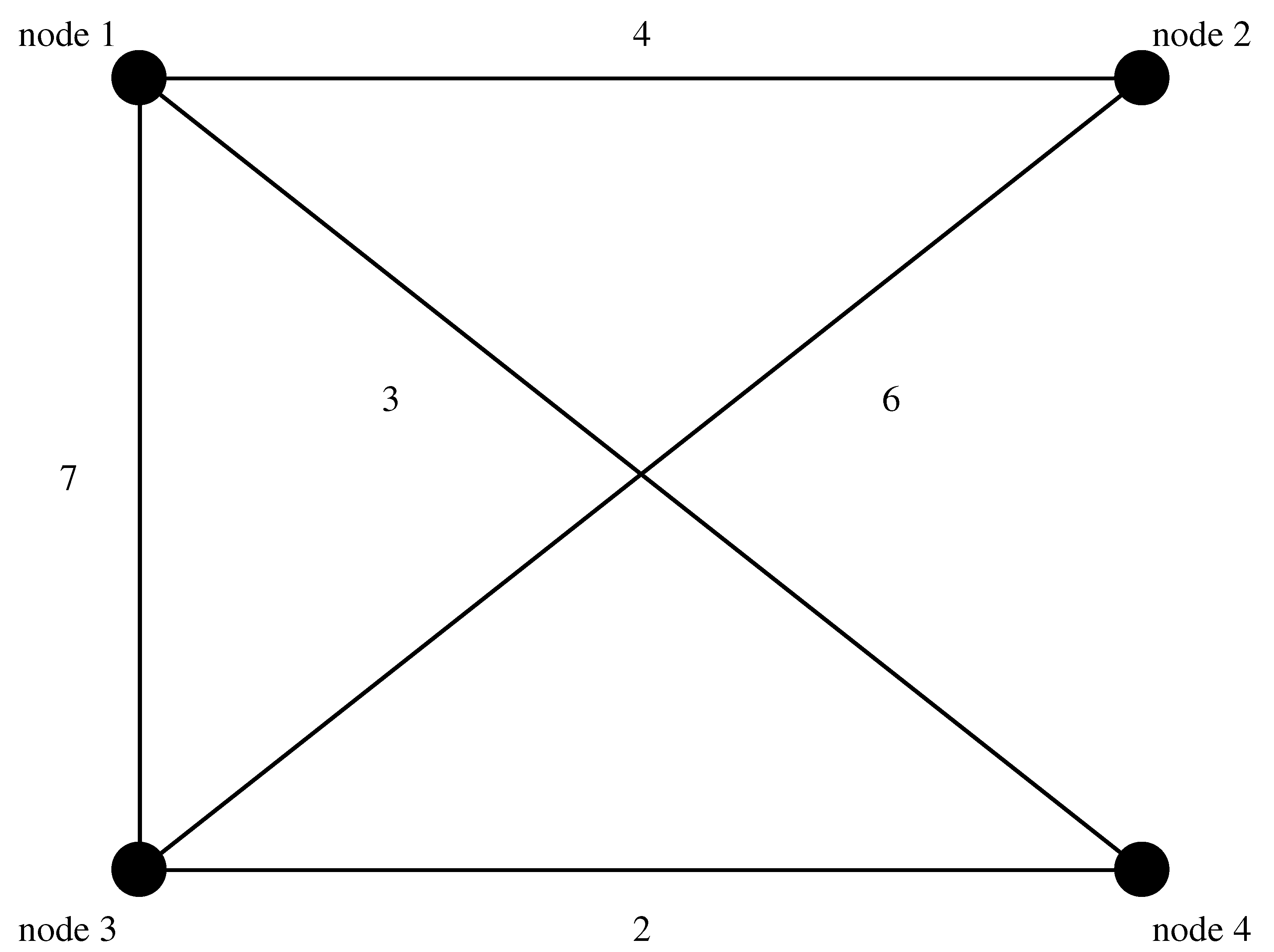
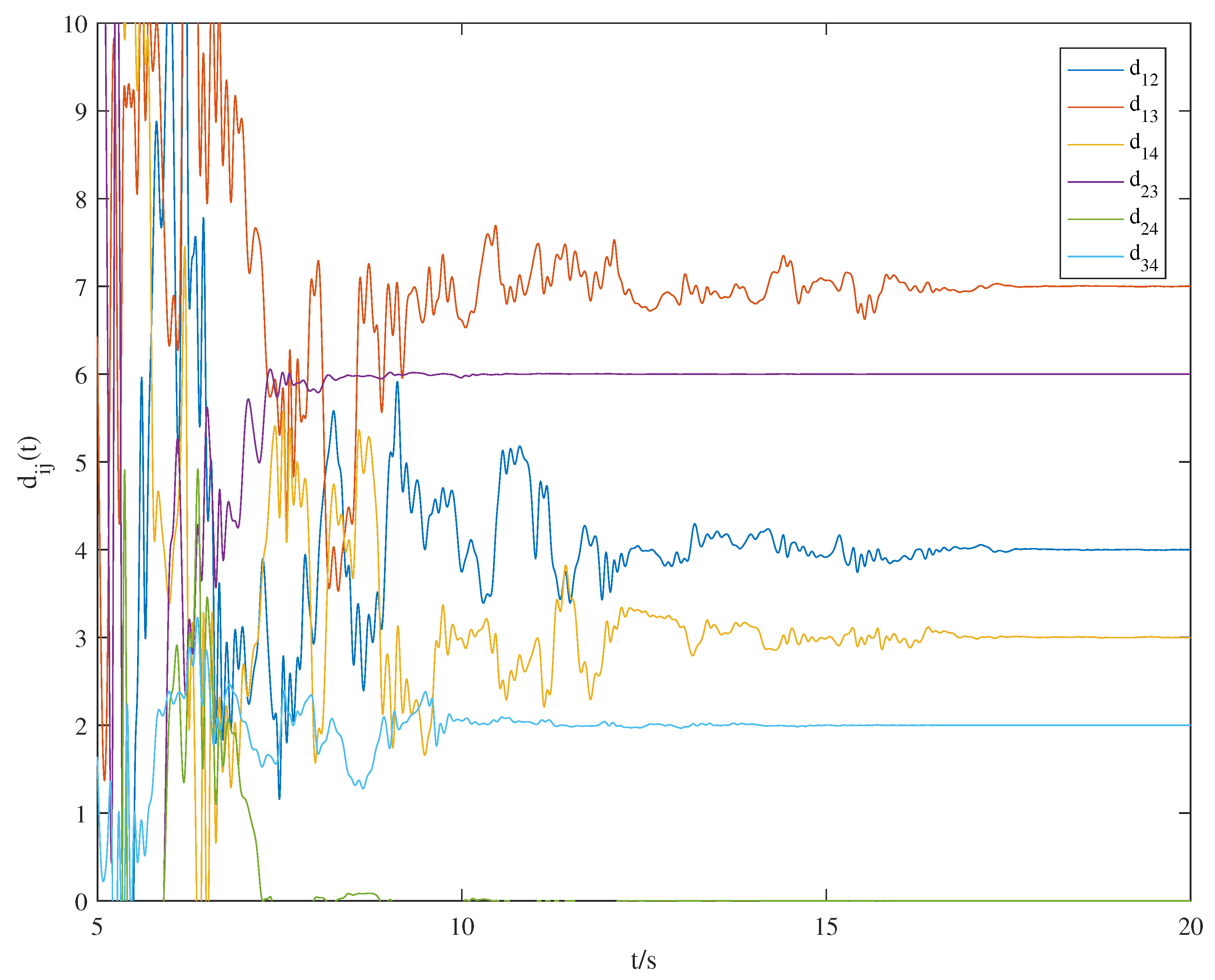
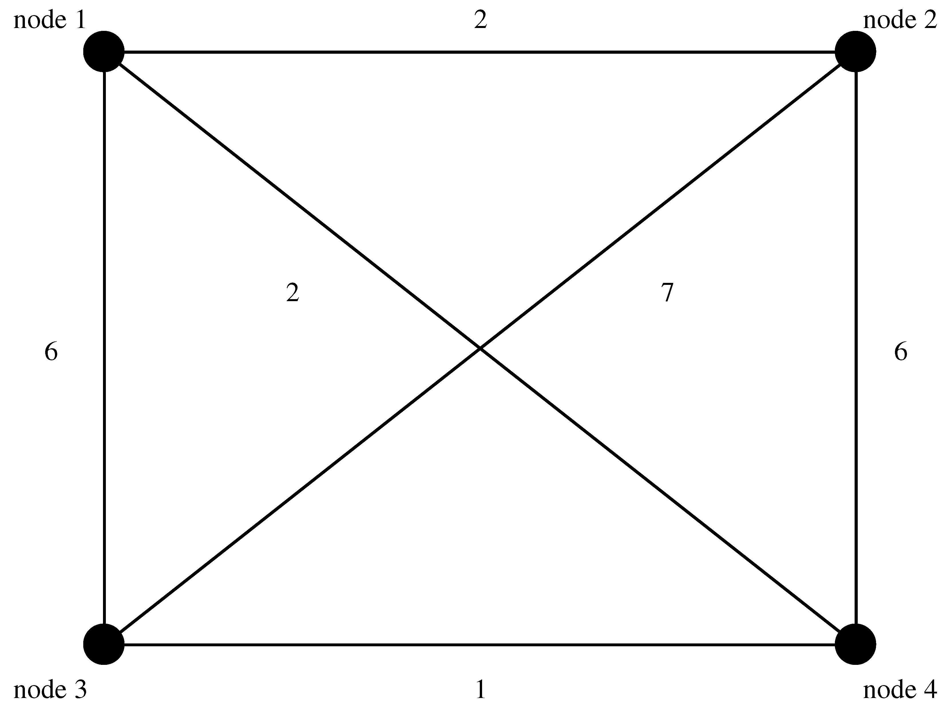
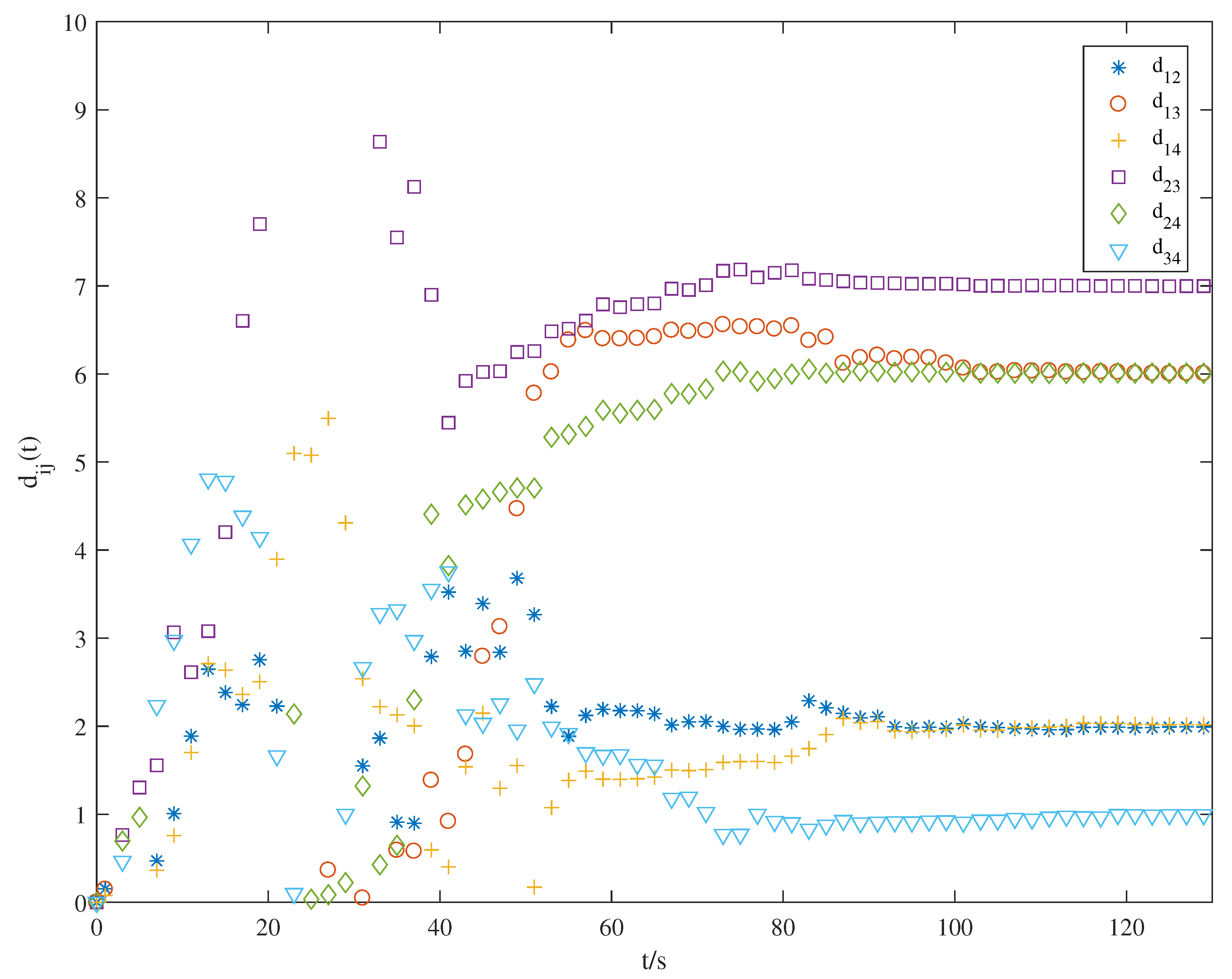
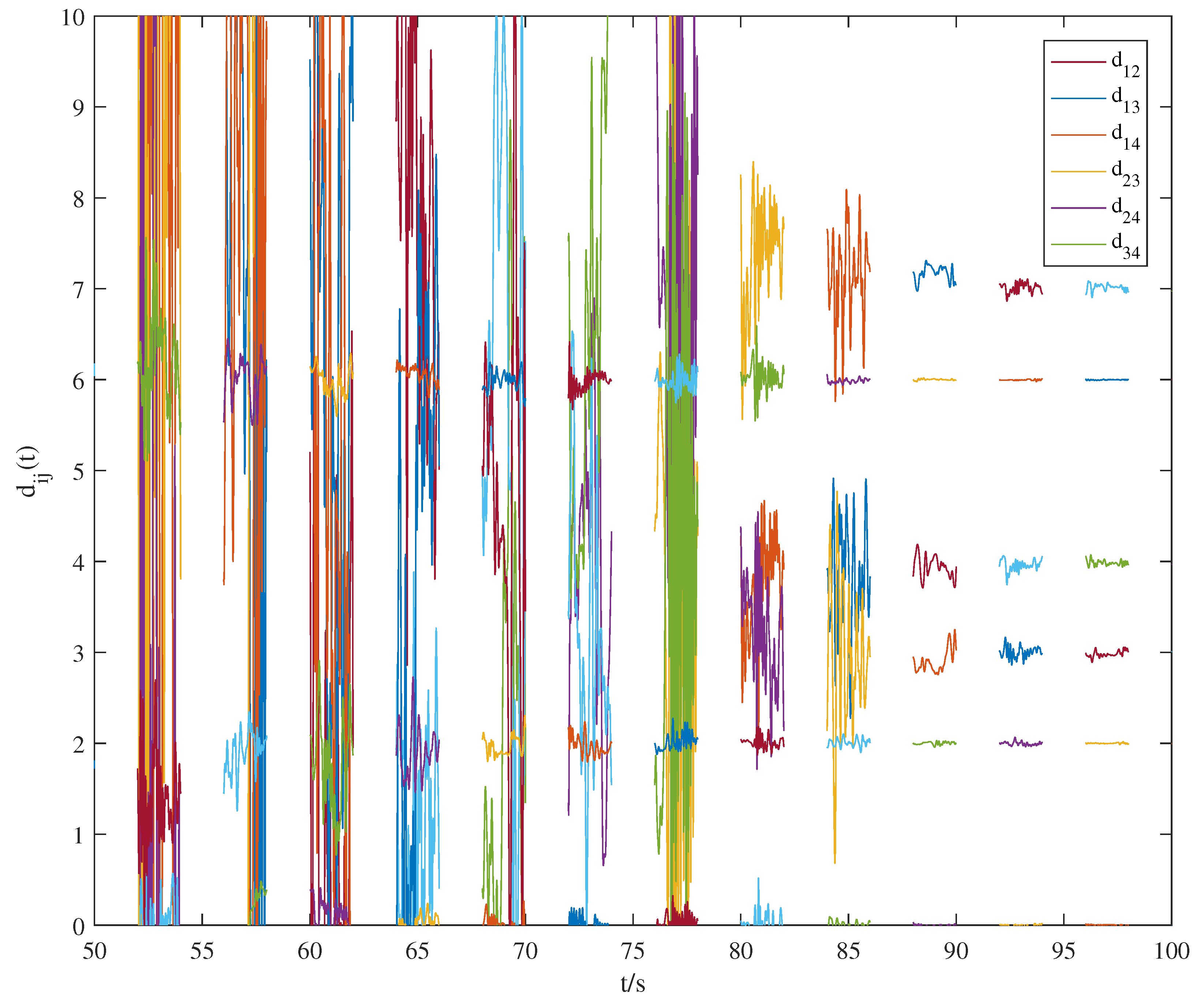
5. Numerical Examples

In this section, three numerical examples with different time scales are given to verify our theoretical results. Precisely, examples show how the topology of dynamical networks are identified with T = R , T = h Z and T = j = 0 j ( a + b ) , j ( a + b ) + a , a , b > 0 , respectively. For simplicity, we consider the networks consisting of four identical dynamical nodes. Without loss of generality, the inner coupling function is simplified as h ( x j ) = x j and the coefficient of adaptive controller is set as k i = 1 , i = 1 , 2 , , N . All examples are simulated by random initial values. We can find the appropriate ζ , such that ζ α 2 + β 2 = 1 .
Example 1.
In this example, we consider the continuous case and suppose T = R , such that μ ( t ) 0 . The chaotic Chen oscillator is taken to simulate each node of the network: for i = 1 , 2 , 3 , 4 , f ( x i ) = 35 ( x i 2 x i 1 ) ; 7 x i 1 x i 1 x i 3 + 28 x i 2 ; x i 1 x i 2 3 x i 3 . The unknown outer coupling matrix C is preset to c 1 , 2 = c 2 , 1 = 4 , c 1 , 3 = c 3 , 1 = 7 , c 1 , 4 = c 4 , 1 = 3 , c 2 , 3 = c 3 , 2 = 6 , c 2 , 4 = c 4 , 2 = 0 , c 3 , 4 = c 4 , 3 = 2 . The topology structure is shown in Figure 1. According to Remark 1, we have θ ( t ) > 1 . Therefore, the conditions in Theorem 1 can be satisfied when θ ( t ) ( 1 , 0 ) . Figure 2 shows the results of our simulation when T = R . As can be seen, the estimated value d i j continuously approaches the preset value c i j without additional control. The network topology is successfully identified.
Example 2.
In this example, we consider the discrete case and suppose T = 2 Z , such that μ ( t ) 2 . The chaotic Hénon map is taken to simulate each node of the network: For i = 1 , 2 , 3 , 4 , f ( x i ) = 1 + x i 2 1.4 x i 1 2 ; 0.3 x i 1 . The unknown outer coupling matrix C is preset to c 1 , 2 = c 2 , 1 = 2 , c 1 , 3 = c 3 , 1 = 6 , c 1 , 4 = c 4 , 1 = 2 , c 2 , 3 = c 3 , 2 = 7 , c 2 , 4 = c 4 , 2 = 6 , c 3 , 4 = c 4 , 3 = 1 . The topology structure is shown in Figure 3. According to Remark 1, we have θ ( t ) > 1 . From (18), if we choose B i ( t ) = diag ( 0.88 , 0.88 ) , i = 1 , 2 , 3 , 4 , θ = 2 and δ = 1.27 , then we have Δ 2.0008 . Without loss of generality, we choose Δ = 2 . Figure 4 shows the results of our simulation when T = 2 Z . As can be seen, the estimated value d i j approaches the actual value c i j discretely with impulsive control every 2 s. The network topology is successfully identified.
Example 3.
In this example, we suppose T = j = 0 j ( a + b ) , j ( a + b ) + a , a , b > 0 . Specifically, we let a = 2 and b = 2 then T = j = 0 4 j , 4 j + 2 . The graininess function of T is given by
μ ( t ) = 0 , if t j = 0 4 j , 4 j + 2 , 2 , if t j = 0 { 4 j + 2 } .
We consider the same unknown outer coupling matrix C as indicated in Example 1. The chaotic Chen oscillator is taken to simulate each node of the network: For i = 1 , 2 , 3 , 4 , f ( x i ) = 10 ( x i 2 x i 1 ) ; 28 x i 1 x i 1 x i 3 x i 2 ; x i 1 x i 2 8 3 x i 3 . In this case, θ ( t ) can be chosen by any value between 1 and 0 when μ ( t ) = 0 . When μ ( t ) = 2 , θ ( t ) > 1 . From (18), if we choose B i ( t ) = diag ( 0.88 , 0.88 , 0.88 ) , i = 1 , 2 , 3 , 4 , θ = 2 and δ = 1.1 , then we have Δ [ 2.0726 ] = 2 , which means that impulsive control occurs at each time point of multiples of 2. Figure 5 shows the results of our simulation for this case. As can be seen, the estimated value d i j approaches the preset value c i j intermittently with impulsive control every 2 s. The network topology is successfully identified.

6. Conclusions

In this paper, a topology identification problem of complex dynamical networks on different time scales is studied. We have investigated the outer synchronization between the original network and the auxiliary network on time scales. General synchronization criteria have been proposed according to the matrix inequality and time scale regressive condition. Moreover, we have applied the adaptive controller on the original network and taken the impulsive method to synchronize with the auxiliary chaotic network. An impulsive criterion has been derived to ensure the outer synchronization. Three examples on different time scales have been given to verify our results. The proposed ideas and methods can be extended to the topology identification problem of other complex networks.

Author Contributions

Data curation, Y.P.; Formal analysis, C.C.; Supervision, D.P. All authors have read and agreed to the published version of the manuscript.

Funding

This research was funded by National Science and Technology Innovation 2030-Key Project of “New Generation Artificial Intelligence” of grant number 2021ZD0113103; The Natural Science Foundation of Jiangsu Provincial Higher Education of grant number 19KJB520008; “Qing-Lan Engineering” Foundation of Jiangsu Higher Education Institutions and The high-level talents Training Fund of the fifth “333 Project” of Jiangsu Province; Basic and Applied Research Foundation of Guangdong Province of grant number 2020A1515110996; National Natural Science Foundation of China of grant number 12101139; Special Fund for Scientific Research Talents of GPNU of grant number 2021SDKYA070.

Institutional Review Board Statement

Not applicable.

Informed Consent Statement

Not applicable.

Data Availability Statement

Not applicable.

Conflicts of Interest

The authors declare no conflict of interest.

References

  1. Boccaletti, S.; Latora, V.; Moreno, Y.; Chavez, M.; Hwang, D.U. Complex networks: Structure and dynamics. Phys. Rep. 2006, 424, 175–308. [Google Scholar] [CrossRef]
  2. Schöll, E. Synchronization patterns and chimera states in complex networks: Interplay of topology and dynamics. Eur. Phys. J. Spec. Top. 2016, 225, 891–919. [Google Scholar] [CrossRef]
  3. Lü, L.; Chen, D.; Ren, X.L.; Zhang, Q.M.; Zhang, Y.C.; Zhou, T. Vital nodes identification in complex networks. Phys. Rep. 2016, 650, 1–63. [Google Scholar] [CrossRef] [Green Version]
  4. Zañudo, J.G.T.; Yang, G.; Albert, R. Structure-based control of complex networks with nonlinear dynamics. Proc. Natl. Acad. Sci. USA 2017, 114, 7234–7239. [Google Scholar] [CrossRef] [Green Version]
  5. Zhao, J.; Li, Q.; Lu, J.A.; Jiang, Z.P. Topology identification of complex dynamical networks. Chaos Interdiscip. J. Nonlinear Sci. 2010, 20, 023119. [Google Scholar] [CrossRef] [Green Version]
  6. Peng, H.; Li, L.; Kurths, J.; Li, S.; Yang, Y. Topology identification of complex network via chaotic ant swarm algorithm. Math. Probl. Eng. 2013, 2013, 401983. [Google Scholar] [CrossRef]
  7. Chen, J.; Lu, J.; Zhou, J. Topology identification of complex networks from noisy time series using ROC curve analysis. Nonlinear Dyn. 2014, 75, 761–768. [Google Scholar] [CrossRef]
  8. Yu, D.; Righero, M.; Kocarev, L. Estimating topology of networks. Phys. Rev. Lett. 2006, 97, 188701. [Google Scholar] [CrossRef] [Green Version]
  9. Zhou, J.; Lu, J.A. Topology identification of weighted complex dynamical networks. Phys. A Stat. Mech. Appl. 2007, 386, 481–491. [Google Scholar] [CrossRef]
  10. Zhao, X.; Zhou, J.; Zhu, S.; Ma, C.; Lu, J.A. Topology identification of multiplex delayed networks. IEEE Trans. Circuits Syst. II Express Briefs 2019, 67, 290–294. [Google Scholar] [CrossRef]
  11. Hai, X.; Yu, Y. Topology Identification of Fractional Complex Networks with An Auxiliary Network. IFAC-PapersOnLine 2020, 53, 3675–3682. [Google Scholar] [CrossRef]
  12. Liu, H.; Lu, J.; Lu, J. Topology identification of an uncertain general complex dynamical network. In Proceedings of the 2008 IEEE International Symposium on Circuits and Systems, Seattle, WA, USA, 18–21 May 2008; pp. 109–112. [Google Scholar]
  13. Zheng, Y.; Wu, X.; He, G.; Wang, W. Topology identification of fractional-order complex dynamical networks based on auxiliary-system approach. Chaos Interdiscip. J. Nonlinear Sci. 2021, 31, 043125. [Google Scholar] [CrossRef] [PubMed]
  14. Si, G.; Sun, Z.; Zhang, H.; Zhang, Y. Parameter estimation and topology identification of uncertain fractional order complex networks. Commun. Nonlinear Sci. Numer. Simul. 2012, 17, 5158–5171. [Google Scholar] [CrossRef]
  15. Wang, Y.; Wu, X.; Lü, J.; Lu, J.a.; D’Souza, R.M. Topology identification in two-layer complex dynamical networks. IEEE Trans. Netw. Sci. Eng. 2018, 7, 538–548. [Google Scholar] [CrossRef]
  16. Xu, Y.; Zhou, W.; Fang, J. Topology identification of the modified complex dynamical network with non-delayed and delayed coupling. Nonlinear Dyn. 2012, 68, 195–205. [Google Scholar] [CrossRef]
  17. Tu, C.; Cheng, Y.; Chen, K. Estimating the varying topology of discrete-time dynamical networks with noise. Cent. Eur. J. Phys. 2013, 11, 1045–1055. [Google Scholar] [CrossRef]
  18. Zhao, J.; Aziz-Alaoui, M.; Bertelle, C.; Corson, N. Sinusoidal disturbance induced topology identification of Hindmarsh-Rose neural networks. Sci. China Inf. Sci. 2016, 59, 1–9. [Google Scholar] [CrossRef]
  19. Zhang, H.; Wang, X.Y.; Lin, X.H. Topology identification and module–phase synchronization of neural network with time delay. IEEE Trans. Syst. Man Cybern. Syst. 2016, 47, 885–892. [Google Scholar] [CrossRef]
  20. Wang, L.; Zhang, J.; Sun, W. Adaptive outer synchronization and topology identification between two complex dynamical networks with time-varying delay and disturbance. IMA J. Math. Control Inf. 2019, 36, 949–961. [Google Scholar] [CrossRef]
  21. Zhang, S.; Wu, X.; Lu, J.A.; Feng, H.; Lu, J. Topology identification of complex dynamical networks based on generalized outer synchronization. In Proceedings of the 33rd Chinese Control Conference, Nanjing, China, 28–30 July 2014; pp. 2763–2767. [Google Scholar]
  22. Che, Y.; Li, R.; Han, C.; Cui, S.; Wang, J.; Wei, X.; Deng, B. Topology identification of uncertain nonlinearly coupled complex networks with delays based on anticipatory synchronization. Chaos Interdiscip. J. Nonlinear Sci. 2013, 23, 013127. [Google Scholar] [CrossRef] [Green Version]
  23. Xu, Y.; Zhou, W.; Sun, W.; Pan, L. Topology identification and adaptive synchronization of uncertain complex networks with non-derivative and derivative coupling. J. Frankl. Inst. 2010, 347, 1566–1576. [Google Scholar] [CrossRef]
  24. Yu, D. Estimating the topology of complex dynamical networks by steady state control: Generality and limitation. Automatica 2010, 46, 2035–2040. [Google Scholar] [CrossRef]
  25. Zhang, Q.; Luo, J.; Wan, L. Parameter identification and synchronization of uncertain general complex networks via adaptive-impulsive control. Nonlinear Dyn. 2013, 71, 353–359. [Google Scholar] [CrossRef]
  26. Zhu, S.; Zhou, J.; Lu, J.a. Identifying partial topology of complex dynamical networks via a pinning mechanism. Chaos Interdiscip. J. Nonlinear Sci. 2018, 28, 043108. [Google Scholar] [CrossRef] [PubMed]
  27. Chen, L.; Lu, J.a.; Chi, K.T. Synchronization: An obstacle to identification of network topology. IEEE Trans. Circuits Syst. II Express Briefs 2009, 56, 310–314. [Google Scholar] [CrossRef]
  28. Zhu, S.; Zhou, J.; Chen, G.; Lu, J.A. A new method for topology identification of complex dynamical networks. IEEE Trans. Cybern. 2019, 51, 2224–2231. [Google Scholar] [CrossRef]
  29. Liu, H.; Li, Y.; Li, Z.; Lü, J.; Lu, J.A. Topology Identification of Multilink Complex Dynamical Networks via Adaptive Observers Incorporating Chaotic Exosignals. IEEE Trans. Cybern. 2021. [Google Scholar] [CrossRef]
  30. Cheng, Q.; Cao, J. Global synchronization of complex networks with discrete time delays on time scales. Discret. Dyn. Nat. Soc. 2011, 2011, 287670. [Google Scholar] [CrossRef]
  31. Chen, X.; Song, Q. Global stability of complex-valued neural networks with both leakage time delay and discrete time delay on time scales. Neurocomputing 2013, 121, 254–264. [Google Scholar] [CrossRef]
  32. Liu, X.; Zhang, K. Synchronization of linear dynamical networks on time scales: Pinning control via delayed impulses. Automatica 2016, 72, 147–152. [Google Scholar] [CrossRef]
  33. Ogulenko, A. Asymptotical properties of social network dynamics on time scales. J. Comput. Appl. Math. 2017, 319, 413–422. [Google Scholar] [CrossRef] [Green Version]
  34. Huang, Z.; Cao, J.; Raffoul, Y.N. Hilger-type impulsive differential inequality and its application to impulsive synchronization of delayed complex networks on time scales. Sci. China Inf. Sci. 2018, 61, 1–3. [Google Scholar] [CrossRef]
  35. Wang, B.; Zhang, Y.; Zhang, B. Exponential synchronization of nonlinear complex networks via intermittent pinning control on time scales. Nonlinear Anal. Hybrid Syst. 2020, 37, 100903. [Google Scholar] [CrossRef]
  36. Ali, M.S.; Yogambigai, J. Synchronization of complex dynamical networks with hybrid coupling delays on time scales by handling multitude Kronecker product terms. Appl. Math. Comput. 2016, 291, 244–258. [Google Scholar]
  37. Xiao, Q.; Lewis, F.L.; Zeng, Z. Event-based time-interval pinning control for complex networks on time scales and applications. IEEE Trans. Ind. Electron. 2018, 65, 8797–8808. [Google Scholar] [CrossRef]
  38. Pei, Y.; Bohner, M.; Pi, D. Impulsive synchronization of time-scales complex networks with time-varying topology. Commun. Nonlinear Sci. Numer. Simul. 2020, 80, 104981. [Google Scholar] [CrossRef]
  39. Cheng, Q.; Cao, J. Synchronization of complex dynamical networks with discrete time delays on time scales. Neurocomputing 2015, 151, 729–736. [Google Scholar] [CrossRef]
  40. Bohner, M.; Peterson, A. Dynamic Equations on Time Scales: An Introduction with Applications; Birkhäuser Boston, Inc.: Boston, MA, USA, 2001; 358p. [Google Scholar] [CrossRef] [Green Version]
  41. Bohner, M.; Peterson, A.C. Advances in Dynamic Equations on Time Scales; Springer Science & Business Media: Berlin, Germany, 2002. [Google Scholar]
  42. Boyd, S.; El Ghaoui, L.; Feron, E.; Balakrishnan, V. Linear Matrix Inequalities in System and Control Theory; SIAM: Philadelphia, PA, USA, 1994. [Google Scholar]
Figure 1. Topology structure of the dynamical network in Example 1 and 3.
Mathematics 10 01755 g001
Figure 2. Topology identification for the dynamical network in Example 1.
Mathematics 10 01755 g002
Figure 3. Topology structure of the dynamical network in Example 2.
Mathematics 10 01755 g003
Figure 4. Topology identification for the dynamical network in Example 2.
Mathematics 10 01755 g004
Figure 5. Topology identification for the dynamical network in Example 3.
Mathematics 10 01755 g005
Publisher’s Note: MDPI stays neutral with regard to jurisdictional claims in published maps and institutional affiliations.

