Article

Does Higher Education Level the Playing Field? Socio-Economic Differences in Graduate Earnings

by
Claire Crawford
1,2,* and
Laura Van der Erve
2,3
1
Department of Economics, University of Warwick, Coventry, CV4 7AL, UK
2
Institute for Fiscal Studies, 7 Ridgmount Street, London, WC1E 7AE, UK
3
St Edmund Hall, University of Oxford, Queens Lane, Oxford, OX1 4AR, UK
*
Author to whom correspondence should be addressed.
Educ. Sci. 2015, 5(4), 380-412; https://doi.org/10.3390/educsci5040380
Submission received: 5 October 2015 / Accepted: 4 December 2015 / Published: 11 December 2015
(This article belongs to the Special Issue Widening Participation in Higher Education)

Abstract

:
Education—and in particular higher education—is often regarded as a route to social mobility. For this to be the case, however, the link between family background and adult outcomes must be broken (or at least reduced) once we take account of an individual’s education history. This paper provides new evidence on differences in graduates’ earnings by socio-economic background, exploiting rich individual-level data to account for more of the ways in which graduates from different socio-economic backgrounds differ from each other than has been possible in previous research on this topic. We continue to find significant differences between the earnings of graduates from lower and higher socio-economic backgrounds, even after accounting for a rich array of characteristics, skills and experiences from before individuals went to university, as well as their labour market experiences subsequently. These results suggest that it is not enough simply to encourage more young people to go to university, or even to ensure that they graduate with “good” degrees; policymakers interested in increasing social mobility also need to focus on what happens to them once they leave university to ensure that higher education is truly able to “level the playing field” between those from different socio-economic backgrounds.

1. Introduction

Increasing social mobility has emerged as a key goal of government policy in the UK and US in recent years, largely in response to research that has found substantial social immobility in both countries [1,2,3]. Previous research has highlighted the important role that education can play in “levelling the playing field” (e.g., [4]), hence the extent to which young people from disadvantaged backgrounds can access and perform well in different levels of education is of keen policy interest (e.g., [5]).
Yet the role that education can potentially play in driving social mobility may be weakened if there remains a link between family background and adult outcomes, even once we account for attainment at school and university. Theoretically, there may be a number of reasons why there is a relationship between family background and labour market outcomes, even amongst those with similar educational qualifications. Economic theory would suggest that individuals from more advantaged backgrounds have greater levels of parental investment, giving rise to higher levels of skills only partially reflected in educational attainment, such as non-cognitive or social skills (e.g., [6]). Equally, some sociological theories (e.g., [7]) would suggest that educational attainment is insufficient in and of itself to secure the same occupational status and labour market success for disadvantaged students as for those from more advantaged backgrounds. This is because students from lower socio-economic backgrounds may lack other forms of capital, such as social capital, and hence are less likely to succeed in the labour market as a result.
There has, however, been relatively little research to date in the UK on the extent to which there remain differences in earnings between individuals with similar educational qualifications, and—more importantly—what explains these gaps. This paper seeks to contribute to this literature, focusing on a group of particular academic and policy interest: university graduates. Our aim is to add to the limited previous evidence on the relationship between graduates’ socio-economic background and earnings in the UK, taking advantage of rich individual-level data. This data enables us to provide a fuller picture of the differences in earnings by socio-economic background, including by social class, income and education, and how it changes over time. It also enables us to account for more of the ways in which graduates from different socio-economic backgrounds differ from each other—including some proxies for cultural and social capital—thus enabling us to reduce the extent to which unobserved heterogeneity may be responsible for any remaining significant differences in earnings between individuals from higher and lower socio-economic backgrounds.
Using data from the British Cohort Study (BCS)—a cohort of individuals born in a particular week of April 1970—we explore differences in graduate earnings, focusing on age 26 to minimise the effects of attrition, as well as the selection of individuals into (full-time) work as a result of family formation decisions. In the absence of exogenous variation in socio-economic background—such as that produced by “shocks” to income or variation in school leaving age policies—the estimates we report cannot be interpreted as causal effects of socio-economic status on earnings; instead we regard the groups of characteristics that we add to our models as “transmission mechanisms”, providing insight into the routes through which the environment in which you grow up influences your earnings.
In contrast to previous research—which has tended to focus on differences in earnings on the basis of a single measure of socio-economic status (e.g., [1,8,9], all focus on social class)—we include measures of social class, family income and parents’ education in our model. We also focus on individuals from the highest socio-economic backgrounds compared to those from all other socio-economic backgrounds, as previous research has suggested that there are significant differences in access to elite universities and professional occupations between these groups (e.g., [9,10]), and there is growing interest in how policy can be used to overcome the “hoarding” of opportunities amongst those from the most privileged backgrounds (e.g. [11,12]). Our findings suggest that being from a family with high occupational status, high education and/or high income are all significantly associated with graduate earnings at age 26, implying that there may be a plethora of routes through which being raised in a socio-economically advantaged family confers labour market benefits.
Previous research (e.g., [8,9]) has hypothesised that one reason why there might remain significant differences in earnings between graduates from different socio-economic backgrounds—even amongst those studying the same subjects at the same institutions and who entered with comparable overall A-level attainment and ended up with the same degree class—is that we may not be fully capturing the skills and experiences with which these individuals enter university. These experiences might include the environment in which individuals have been raised and hence some elements of the social and cultural capital with which they are endowed. If it is the case that individuals from higher socio-economic backgrounds have capital that individuals from lower socio-economic backgrounds lack, on average, then this might help to explain the differences in earnings that we see.
Using the rich data to which we have access in the BCS, we explore the extent to which such skills and experiences matter. We are not able to consider the role of networks and social capital directly—which might matter particularly for those from the highest socio-economic backgrounds, enabling them to access the most competitive occupations, for example—but other work (e.g., [9]) has suggested that measuring the quality of individuals’ networks and support is difficult in survey data and, as measured, they do not play a major role in explaining differences in earnings amongst graduates. We focus instead on accounting for more detailed information on family background, some proxies for social and cultural capital, and rich measures of cognitive skills at ages 5 and 10 and non-cognitive skills at ages 5, 10 and 16. We also account for a richer set of measures of school attainment at ages 16 and 18—including information on grades and subjects—than has been possible in previous studies. Somewhat surprisingly, the addition of these richer measures of skills and experiences makes very little difference to the remaining gap in earnings between graduates from higher and lower socio-economic backgrounds, suggesting that the factors we are able to measure and account for in the BCS do not play an important role—over and above a parsimonious set of controls for family background and educational attainment—in driving socio-economic differences in graduate earnings.
The largest reductions to our coefficients on socio-economic status occur when we include controls for the individual’s occupation at the time of the survey. This suggests—as has been found by previous research (e.g., [9,13])—that part of the benefit of coming from a higher socio-economic background is to enable individuals to access higher status jobs. However, our findings suggest that there remain some differences in earnings within occupation too.
The fact that we continue to find significant differences between the earnings of graduates from lower and higher socio-economic backgrounds, even after accounting for a rich array of characteristics, skills and experiences from before individuals went to university, as well as their subsequent labour market experience, suggests that higher education is not sufficient to fully “level the playing field” between otherwise-identical individuals from higher and lower socio-economic backgrounds, and thus that there remains a challenge for policymakers interested in the role of higher education as a route to social mobility.
This paper now proceeds as follows: Section 2 briefly discusses previous literature in this area; Section 3 and Section 4 describe our methods and data respectively. Section 5 presents our results, and Section 6 concludes.

2. Previous Literature

Our goal in this paper is to understand whether, if we were to compare two individuals who went to the same university, studied the same subject and achieved the same degree class—but who came from different socio-economic backgrounds—would there be any difference in their earnings? Our paper is therefore associated with two separate but related literatures: on social and intergenerational income mobility and the role of education in mediating these relationships, and on heterogeneity in the returns to education by socio-economic background.
While there is considerable evidence of heterogeneity in degree returns by subject, institution and degree class in the UK (e.g., [14,15,16,17,18]), there is very little evidence on how graduates’ earnings vary by socio-economic background.
Using the same data as we do—the 1970 British Cohort Study—Bratti et al. [19] explore whether the return to having an undergraduate degree varies by family social class (defined as the highest of the father and the mother when the child was aged 10). The authors compare the earnings at age 30 of those who obtain an undergraduate degree with those who have at least two A-levels (or equivalent qualifications), with the analysis run separately for males and females. They find that the return to a degree is 2.7 percentage points lower for males from families in the highest two social class groups relative to males from the lowest social class group (14.1% vs. 16.8%). The returns are also lower for females from higher social classes relative to the lowest social class group, but these estimates are not significantly different from zero. Their results suggest that the return to having a degree varies somewhat by parental social class, but nowhere near as much as by degree subject or class.
There is also some evidence from the UK on the extent to which graduate earnings vary by the type of school attended. For example, Dolton and Vignoles [20] evaluate the impact of attending private school 6 years after graduation amongst those leaving higher education in 1980. They find a private school premium of around 7% for men but no significant differences for women. Similarly, Naylor et al. [21], using data on those leaving university in 1993 and focusing on average occupational earnings (as their data lacks individual wage information) find a 3% wage premium for graduates who had attended a private school, with higher fee private schools giving rise to higher wage premiums for their students.
The international literature on the extent to which degree returns vary by socio-economic background is also sparse. Brand and Xie [22] investigate whether returns are higher or lower for those who are more or less likely to go to college. They find that those who are least likely to go tend to have higher returns than those who are most likely to go. Given the well-established socio-economic differences in the likelihood of going to university in England (e.g., [10,23]), as well as in most other countries, we can hypothesise that their results would suggest higher returns for individuals from lower socio-economic backgrounds, in line with the direction of the point estimates in Bratti et al. [19].
There are also a number of papers which investigate whether the returns to education more generally vary by socio-economic background. For example, using data from the 1972 General Household Survey in the UK, Papanicolaou and Psacharopoulos [24] assess whether the return to an additional year of schooling varies by fathers’ occupation. They find evidence of a negative relationship between occupation and the returns to schooling, i.e. that those whose fathers work in lower occupations benefit more from an additional year of schooling than those whose fathers work in higher occupations. This differs from the results of similar analysis conducted using the Panel Study of Income Dynamics by Cohn and Kiker [25], who find little evidence that the return to an additional year of schooling varies by fathers’ occupation in the United States.
Again using US data, Altonji and Dunn [26] focus on differences in the returns to schooling by parental education rather than occupation. When identification relies on a “selection on observables” approach—as is the case in the papers described above—the authors do not find significant differences in the returns to schooling by parents’ education. However, when they use family fixed effects models—essentially relying on differences in siblings’ schooling to strip out any fixed unobservable family-level differences that might affect wages—they find positive and significant effects of mother’s education on the earnings of both males and females. Exploiting variation in years of schooling between identical twin pairs in the US, Ashenfelter and Rouse [27] similarly find years of schooling interacted with average parental education level to be positively related to earnings (although these estimates are not significantly different from zero). These papers have used approaches which try to overcome the potential endogeneity of schooling choices on the basis of unobserved as well as observed characteristics, which the UK studies generally have not. This may suggest that using different empirical methods might also produce different results in the UK.
The second literature to which our paper relates is that on the link between socio-economic circumstances during childhood and adulthood, and the extent to which education mediates these relationships. There is an extensive literature both in the UK (e.g., [1,4]) and in other countries (e.g., [2,3]), which documents the links between the socio-economic circumstances of parents and children, whether measured by income, education or social class. However, there is less evidence on the extent to which these relationships remain once we account for different educational choices.
Bukodi and Goldthorpe [13] tackle this question from a sociological perspective, investigating the extent to which education—including higher education—influences the chances of individuals going into different social classes, and how this varies over time/across cohorts. They also investigate how these relationships vary by fathers’ social class (measured around age 10/11). To do so they use data from the 1970 British Cohort Study, plus the 1958 National Child Development Study and the 1946 National Survey of Health and Development. They find that having higher educational qualifications is strongly associated with a greater likelihood of being part of the “salariat” (social classes 1 and 2), but that this effect did not vary by fathers’ social class.
Blanden et al. [28] and Blanden et al. [4] use similar data to explore the extent to which the link between cohort members’ earnings in adulthood and family income in childhood is mediated by the inclusion of controls for educational attainment, with a particular focus on the extent to which this can help to explain falls in intergenerational income mobility over time within the UK. Blanden et al. [28] find that controlling for highest educational qualification achieved accounts for 17 percent of the fall in mobility for sons and 28 percent for daughters, highlighting that the expansion of education participation that has been occurring over time in the UK—especially in terms of higher education—has largely benefitted those from higher socio-economic backgrounds. Blanden et al. [4] use slightly richer measures of educational attainment, controlling for the number of O- and A-levels that cohort members hold, as well as their participation in education beyond compulsory school leaving age, finding that these measures jointly account for around a third of the link between family income and sons’ earnings amongst those born in 1970. They additionally explore the role of cognitive and non-cognitive skills measures and early labour market attachment, finding that they collectively account for a further 23% of the gap. Our paper is similar in spirit to Blanden et al. [4], except our focus is on understanding whether similar relationships exist within education groups—specifically, amongst those who graduate from university.
Macmillan et al. [9] and Crawford and Vignoles [8] had similar aims, both using official survey data on the cohort of graduates leaving university in 2006–07 to explore the extent to which socio-economic background continues to influence labour market outcomes, even amongst individuals from the same universities with similar degree outcomes in the same subjects. Macmillan et al. [9] focus on access to ‘top jobs’, finding that, 3.5 years after graduation, those with parents in a top NS-SEC occupation are 4.7 percentage points more likely to be working in a top NS-SEC occupation themselves. Similarly, Crawford and Vignoles [8] find that graduates whose parents work in routine occupations earn around 9% less, on average, than their counterparts whose parents worked in a higher managerial or professional occupation. Both studies find that these differences can be largely explained by the other ways in which graduates from different socio-economic backgrounds differ. They also, however, find unexplained differences in occupational choices and earnings by school type—specifically, whether or not individuals attended a private school, which can be regarded as one route through which other dimensions of socio-economic status (such as income or education) may play out.
This paper adds to the limited empirical evidence from the UK on the extent to which graduates’ labour market outcomes vary by socio-economic background, building on the previous evidence by accounting for a much richer set of characteristics observed before and after university in order to explore the routes through which socio-economic background influences adult earnings. We also show how these relationships change as graduates get older.

3. Methods

We are unable to use an experimental or quasi-experimental approach to estimate differences in earnings by socio-economic background, so we instead rely on richly specified regression models to provide insight into the routes through which the environment in which you grow up influences your earnings.
To do so, we estimate an ordinary least squares regression model of the relationship between various student characteristics and graduates’ earnings. The natural log of annual earnings (Y) of individual i at time t are hypothesised to be a function of various characteristics, skills and experiences garnered throughout childhood and early adulthood, as shown in equation (1):
ln Y i t = β 1 S E S i + β 2 X i + β 3 H i + β 4 S i + β 5 E i t + ε i t
where SESi denotes a vector of controls capturing the individual’s socio-economic background; Xi denotes a set of individual and family background characteristics, including gender, ethnicity, region, parents’ marital status, and so on; Hi denotes the individual’s stock of human capital, including cognitive and non-cognitive skills, and attainment at school and at university; Si denotes the individual’s stock of social and cultural capital, which we try to proxy using measures such as their own and their parents’ aspirations and expectations for the cohort member’s education and career; Eit denotes the individual’s post-university experiences, including measures of labour market attachment and occupation; and ԑit is an individual-level error term.
Our primary interest is in understanding whether there are differences in graduates’ earnings by socio-economic background, and if so, how these gaps are attenuated once we allow for other factors. We start by presenting the results from a model that only controls for the individual’s socio-economic background, and then progressively include a series of measures designed to capture their other characteristics, skills and experiences which might be influenced by socio-economic background and may also affect their earnings. If the addition of these factors reduces the coefficients on socio-economic status, this suggests that they can be regarded as transmission mechanisms for socio-economic background—routes through which it influences earnings. The purpose of this exercise is to provide insight into both the age and area in which policy might potentially be most effective at reducing the influence of socio-economic status on earnings, though as we outlined earlier, our evidence is not causal.
Following the previous UK literature on this topic, we start by comparing graduate earnings by fathers’ social class, before adding in other measures of socio-economic background (specifically family income and mothers’ and fathers’ education) to explore the extent to which other dimensions of socio-economic background matter too. To emphasise the added value of the BCS data (described in more detail in the next section), we next add a parsimonious set of controls similar to those used in previous studies based on administrative data (e.g., [8,9]), before then going on to highlight how much more of the remaining gap we can explain using the richer data at our disposal.
We start by adding other individual and family background characteristics, and various measures of social and cultural capital, to investigate the extent to which other features of the environment in which individuals grow up are one of the routes through which socio-economic status influences earnings. Next we add a rich set of measures of individual skills, starting with various measures of cognitive and non-cognitive skills in early childhood (up to age 10), followed by a detailed set of information about the qualifications, grades and subjects that individuals achieved at the end of secondary school (age 16) and at the end of college (age 18). (These variables are described in more detail in the next section.) The extent to which the addition of these measures reduces the coefficients on socio-economic background provides an indication of how far differences in graduate earnings arise because individuals from higher socio-economic backgrounds enter the labour market with experiences, skills and qualifications which are more desirable to employers than their counterparts from lower socio-economic backgrounds.
Finally we account for more detailed information about individuals’ career preferences and labour market experiences, ending our analysis by including a measure of the individual’s occupation at the time of the survey. We do so in order to investigate the extent to which any differences in earnings that we observe arise as a result of the selection of graduates from different socio-economic backgrounds into different occupations, or whether there remain differences in earnings even conditional on the types of jobs that graduates are doing.
Our main results are estimated on both males and females, but given the literature on gender differences in the graduate labour market (e.g., [29]), the appendix additionally shows the results when we estimate each model separately for males and females.

4. Data

We use data from the British Cohort Study, which tracks individuals born in a particular week of April 1970 through their lives, up to and including the latest survey in 2012, when the individuals were aged 42. The first sweep of the survey contained 17,196 individuals, but our focus is on graduates, of which there are 1711 in the sample at age 26. Moreover, because our main outcome of interest is earnings, we additionally restrict our attention to those who are in work.
In order to maximise the sample at our disposal, we focus on socio-economic differences in earnings at age 26, when there are 1372 graduates in work who report their earnings. (We account for missing data in all other covariates by including missing dummies in our analysis.) When we show how the effect of socio-economic background changes over time (as graduates get older), we focus on a common sample of graduates who remain in work (and in the sample) between ages 26 and 42. This gives us just 511 graduates. These results in particular should therefore be interpreted with some caution since this sample is quite selected and may give rise to biases.
Our main covariates of interest are various measures of socio-economic background, particularly indicators of high socio-economic background. Specifically, we include:
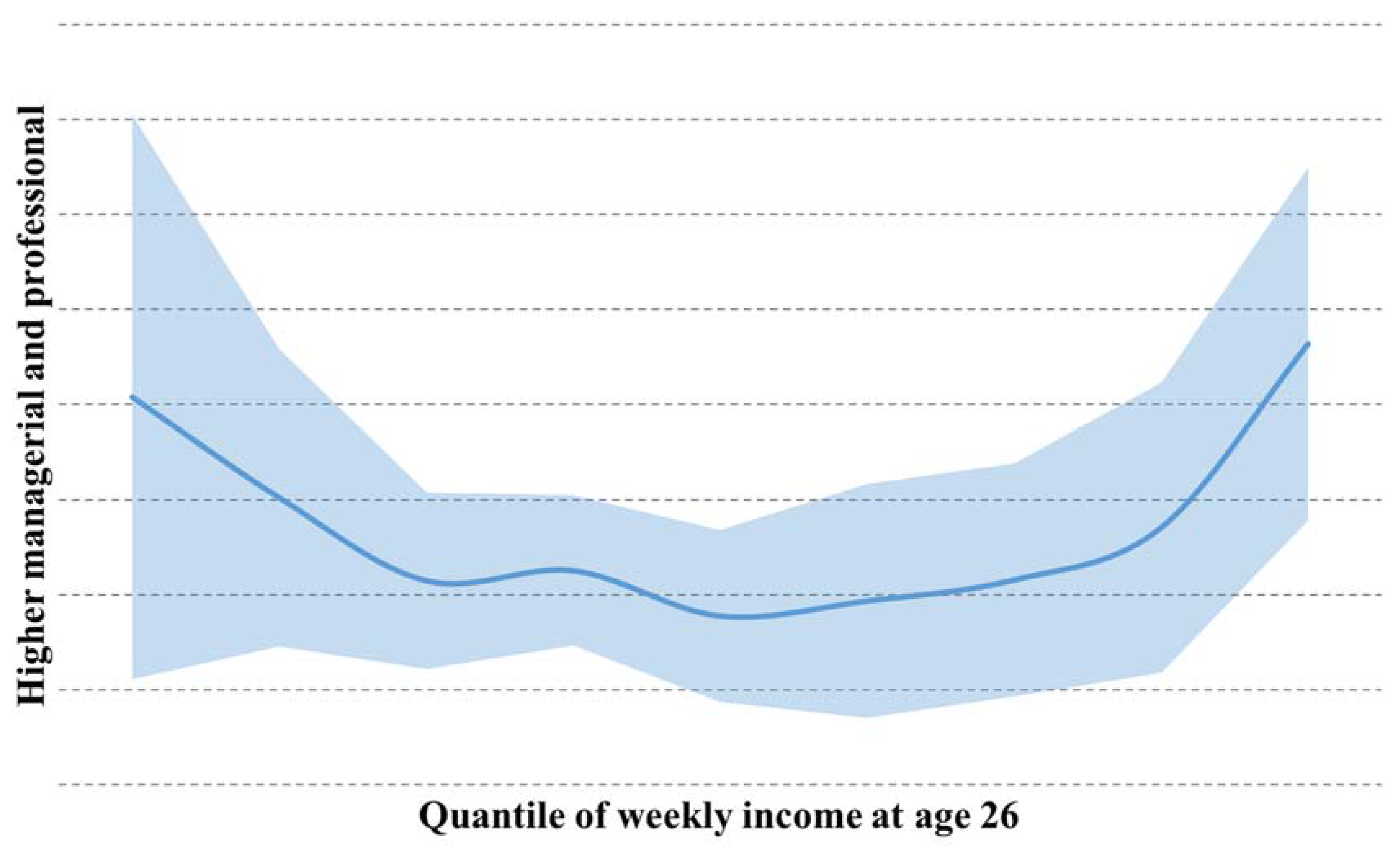
  • Fathers’ social class: we use the NS-SEC measures of social class from when the child was age 10. We include an indicator for being from social class 1—those from higher managerial and professional backgrounds—relative to those from all lower social classes. Around 23% of graduates in our sample at age 26 were from the highest social class group and around 19% were missing this information.
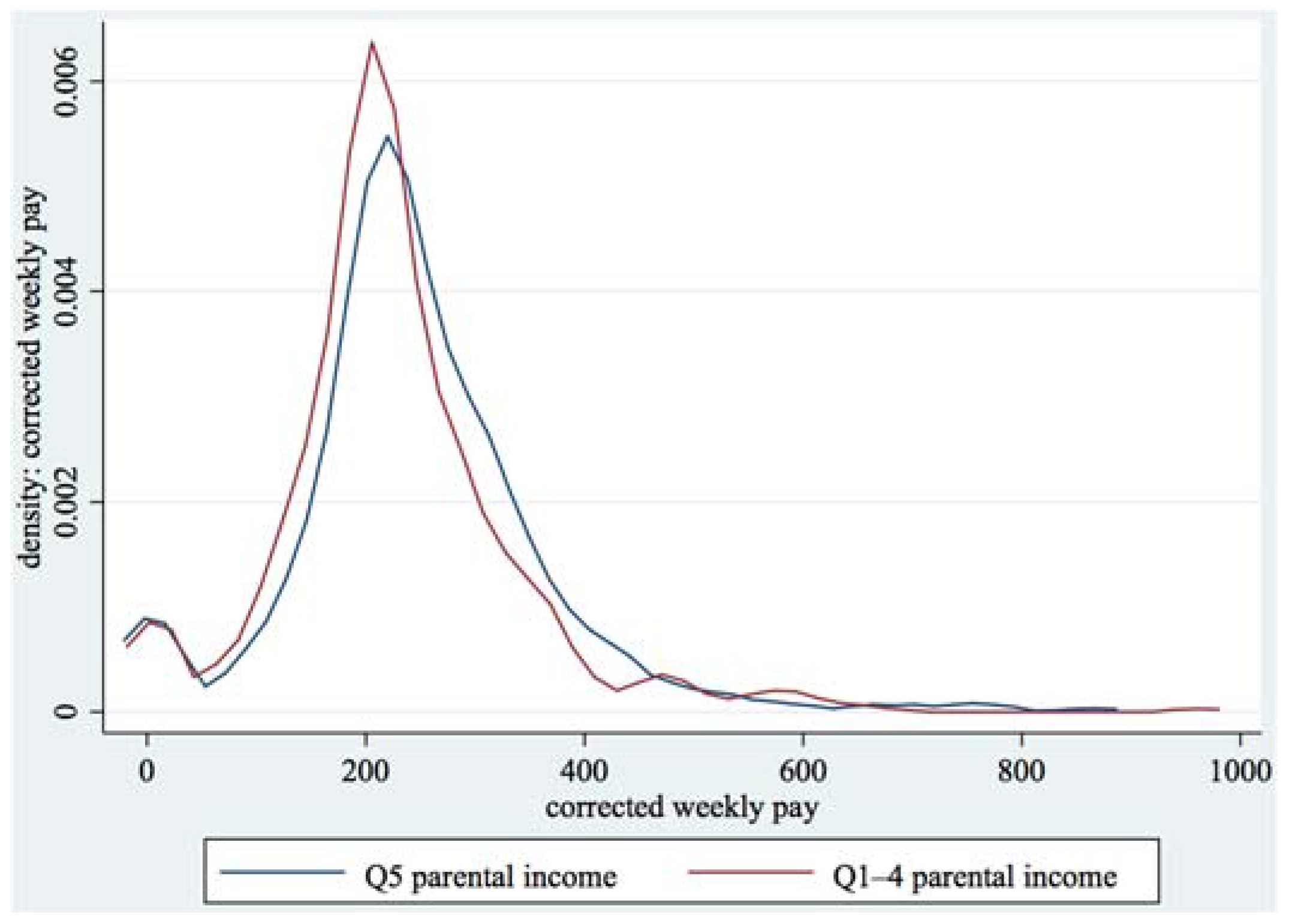
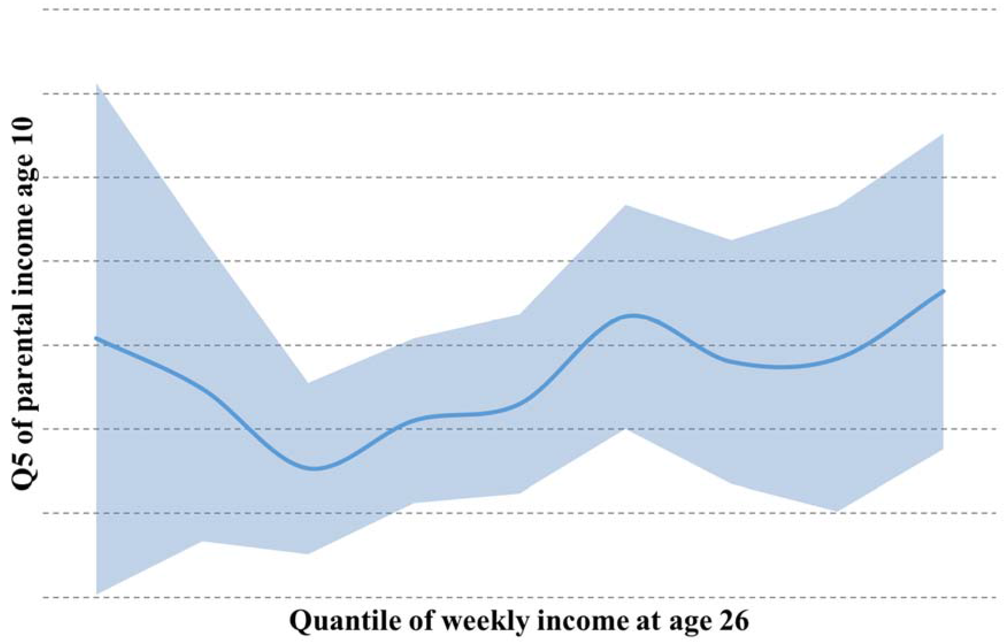
  • Family income: we use a measure of net family income at age 10 created under the auspices of the CLOSER research grant (the acknowledgements section at the end of the paper provides further details). We split individuals into five equally sized groups on the basis of this measure, and include an indicator for being from one of the 20% richest families relative to the remaining 80% of families in our model. Of our 1372 graduates, 211 were from one of these families. (297 did not have information on family income.) The median income of individuals in this top income group was £264 per week in 1980 prices.
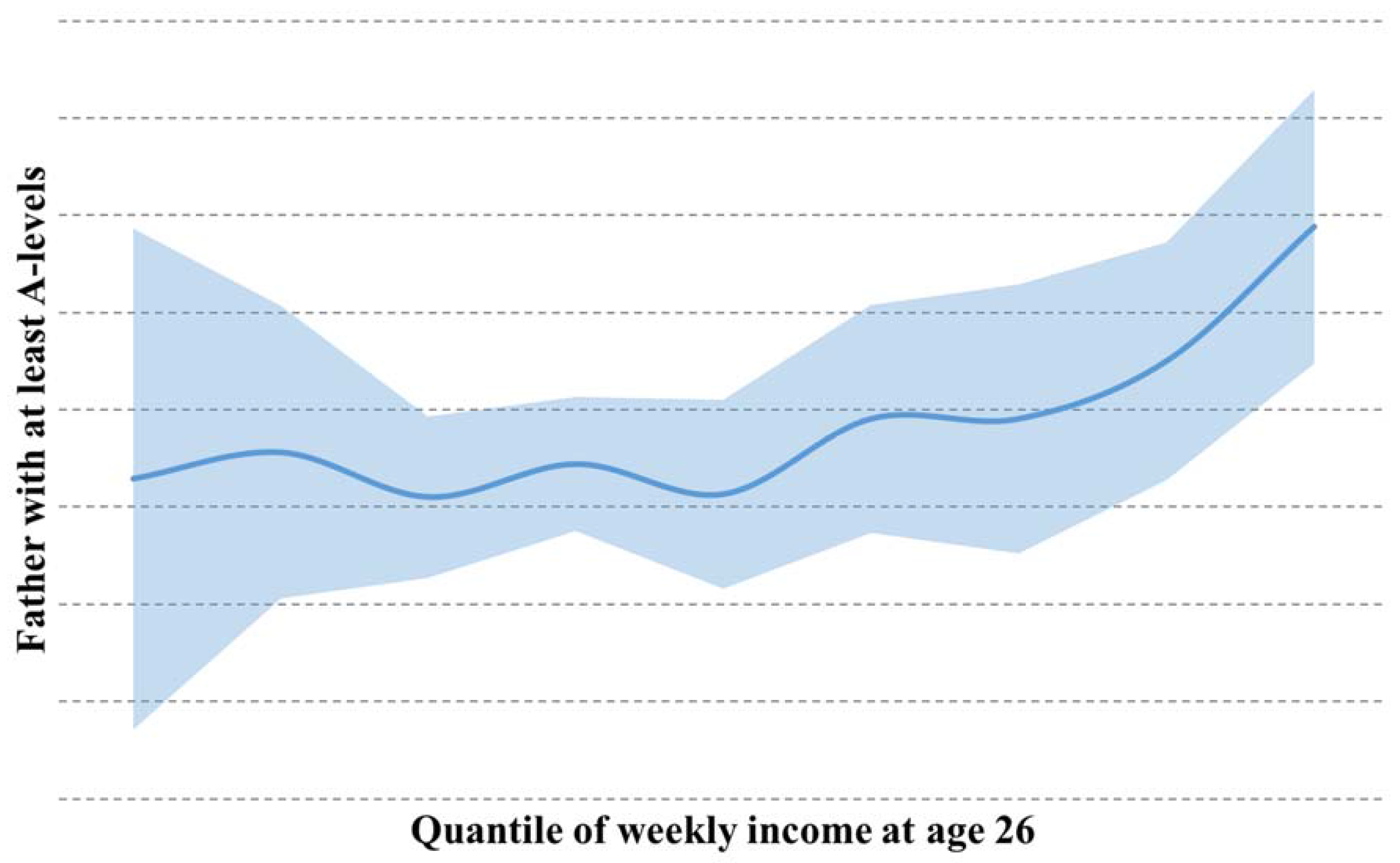
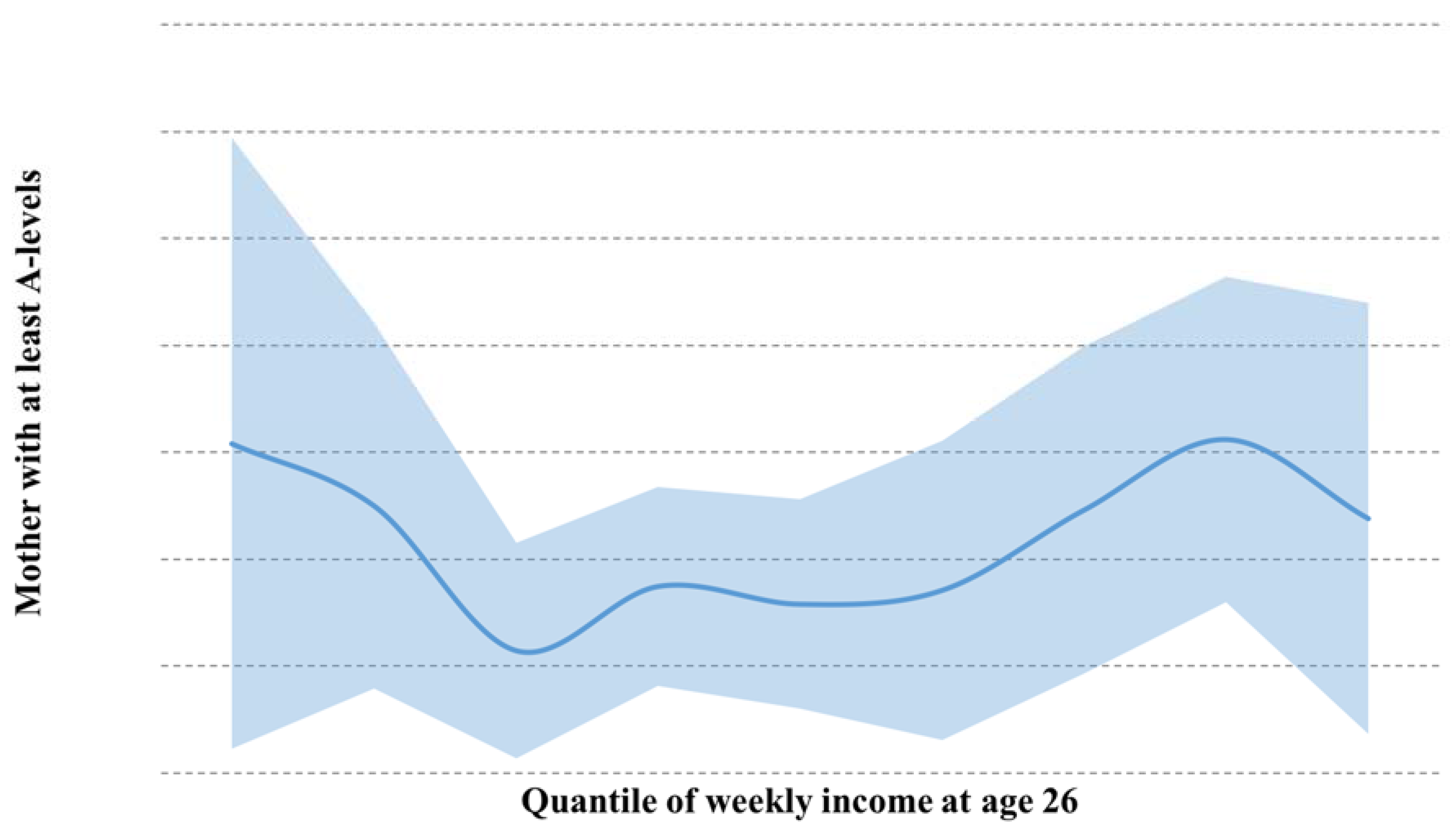
  • Mothers’ and fathers’ education: we use separate indicators for having a mother or a father with at least A-levels (or equivalent qualifications). Around 16% of our sample of graduates had a mother with at least this level of educational attainment, and around 40% had a father with at least this level. Twenty-five percent were missing information on either mothers’ or fathers’ educational attainment.
The factors that explain differences in earnings between individuals from medium and high socio-economic backgrounds, and those from medium and low socio-economic backgrounds, may be quite different. For example, one might imagine that access to networks and financial support to engage in internships might be particularly relevant for individuals at the top of the socio-economic distribution, while knowledge of the range of occupations on offer—and their associated remuneration—may be more relevant in shaping the choices of those at the bottom of the distribution.
Both questions are of clear policy interest. However, we choose to focus on those at the top of the distribution in this paper, as the proportion of individuals from the lowest socio-economic backgrounds who go to university—particularly amongst this older cohort—is relatively small, and one could argue that ensuring more individuals from lower socio-economic backgrounds have the grades to attend and do well at high status universities studying high return subjects may play a greater role in ensuring that higher education contributes to social mobility for those towards the bottom of the distribution, as has been suggested by previous research (e.g., [10,30]). For completeness, however, we show in the appendix what happens if we were to separate out those from the lowest socio-economic backgrounds from those in the middle of the socio-economic distribution. In this analysis, the lowest socio-economic groups are defined as those with fathers working in semi-routine occupations, those in the bottom quintile of the parental income distribution, and those whose mother or father have no education qualifications.
Our main outcome variable is a measure of gross weekly earnings at age 26. Figure 1 shows the distribution of earnings at age 26 amongst graduates by family income, illustrating how it differs between those who grew up in one of the 20% richest families, compared to one of the 80% poorest families. It shows that the distribution of earnings amongst those from the richest families is slightly to the right of the distribution amongst those from poorer families, providing the first evidence that family income may be significantly associated with graduate earnings at age 26. Indeed, median earnings are around £25 per week higher (in 1996 prices) amongst those from the richest 20% of families than those from the poorest 80% of families. The difference is slightly smaller if we compare individuals by fathers’ social class or parental education.
Figure 1. Distribution of gross weekly earnings at age 26, by quintile group of family income. Notes: Q5 represents the 20% of families with the highest income at age 10; Q1–4 represents the remaining 80%.
Education 05 00380 g001
As described above, we begin our analysis by comparing graduate earnings by fathers’ social class. (In separate analysis—available from the authors on request—we use hourly wages rather than weekly earnings, finding that the results do not materially change.) We then add in other measures of socio-economic status to explore the extent to which other dimensions of socio-economic background matter too, before moving on to include a parsimonious set of controls similar to those used in previous studies based on administrative data—specifically gender, ethnicity, region and type of school attended; number of A-levels; and degree class, subject and institution. We take this as our baseline specification, from which we go on to assess the value of the richer data at our disposal.
We do so largely chronologically. We start by including a richer set of family background controls, designed to capture the circumstances in which children were raised. In particular, we include controls for number of siblings, birth order, birth weight, whether the child was born prematurely, the age of the mother at birth, whether the mother was married at birth, and whether both natural parents are present at age 10. We also include a range of measures designed to at least partially proxy for some measures of social and cultural capital, including whether the mother drank or smoked during pregnancy, whether the mother attended antenatal classes, whether the child was ever breastfed, whether the child attended a formal pre-school setting, parental interest in the child’s education, whether they help with homework, and parents’ aspirations for their child’s education.
These factors are designed to capture differences in family stress and investment which previous literature has shown to be mediators for socio-economic status (e.g., [31,32]), and which we confirm exhibit socio-economic gradients. For example, Appendix Table A1 shows that cohort members from the richest 20% of families are nearly seven percentage points more likely to be living with both natural parents by the age of 10 than cohort members from the poorest 80% of families. They are also around nine percentage points more likely to have been breastfed; six percentage points more likely to have been read to daily by their parents at age five; and their parents are around eight percentage points more likely to want them to go to university than parents in the poorest 80% of households.
Next we include measures of cognitive and non-cognitive skills, many of which are standardised to have mean zero and standard deviation one. Where we standardise these measures, we do so across the whole sample at the time the test was taken, meaning that the average amongst our sample need not be zero. We start by including measures of early cognitive skills in our model. Specifically, we use an average of standardised test results in copying, human figure drawing, profile drawing, vocabulary and reading taken at age five (see Parsons [33] for full details of these tests).
We use a variety of measures at age 10, including:
  • An average of standardised scores across four elements of the British Ability Scales (BAS);
  • An average standardised score across three other tests designed to measure language skills, including comprehension, dictation and copying;
  • A standardised score from the CHES Friendly Maths test;
  • A standardised score from the Shortened Edinburgh Reading Test.
We also use a range of measures of non-cognitive skills at ages 5, 10 and 16. Specifically:
  • Indicators for whether the child was deemed to have ‘normal’ behaviour, ‘moderate’ behavioural problems or ‘severe’ behavioural problems based on mother-reported responses to questions from the Rutter Behavioural Scale at ages 5, 10 and 16;
  • A standardised average of scores on the Conners Hyperactivity Scale, as reported by the mother at ages 10 and 16;
  • Standardised scores of teacher-reported behaviour at age 10 about the child’s application, extroversion, hyperactivity and anxiousness;
  • A standardised score from the CARALOC self-reported locus of control scale at ages 10 and 16;
  • A standardised score from the LAWSEQ self-reported scale of self-esteem at ages 10 and 16;
Further details on these measures of cognitive and non-cognitive skills can be found in the appendix.
Compared to most previous studies on this topic, we also control for more detailed information on school achievements. Specifically, we use measures of the number of O-levels at grades A–C and below that each cohort member obtains in facilitating subjects (maths, English, science, humanities and languages) and in other subjects, as reported at age 26. We do the same for the number of A-levels. We also add a couple more school characteristics, namely whether the child attended a grammar school or a single sex school. As shown in Appendix Table A1, there are strong socio-economic gradients in some of these measures, highlighting their potential as transmission mechanisms through which socio-economic background might affect graduates’ wages. For example, individuals from the richest 20% of families have, on average, significantly more O- and A-levels at grades A–C in facilitating subjects than those from the poorest 80% of families; they are also significantly more likely to have attended a single sex school.
Finally, we include a series of measures designed to capture different labour market attitudes and experiences. To understand whether individuals from different socio-economic backgrounds might have different preferences or expectations about their careers, we include responses to questions on whether getting a job is about who or what you know; whether having an interesting and varied job or a high paying job is important to the cohort member; and on whether they would like to go into a professional career. There are some interesting socio-economic differences in these measures. For example, Appendix Table A1 shows that the proportion of individuals reporting that high wages are very important to them in a job is around eight percentage points higher amongst the poorest 80% of graduates than amongst the richest 20% of graduates, while the proportion reporting that they would like to go into a professional occupation is about five percentage points lower amongst those from lower socio-economic backgrounds (although this gap is not significantly different from zero).
We also account for prior labour market attachment. Specifically, we include dummies for whether, by each age, the individual has never been unemployed, has been unemployed for less than three months, between three and six months, or more than six months. We also control for the number of unemployment spells and the number of years they have been in employment. Our final specification controls for the individual’s own social class at the time of the survey, to explore the extent to which socio-economic differences in graduate earnings remain even amongst individuals in similar jobs.

5. Results

Table 1 presents our main results. We start by investigating the extent to which the measure of socio-economic background used may matter for our results. Following the previous UK literature on this topic, Column 1 shows the raw difference in earnings at age 26 between graduates whose father worked in a higher managerial and professional occupation when they were aged 10 and those whose father worked in any other occupation. It shows that, at age 26, graduates from the highest social class earned just under 12% more, on average, than those from other backgrounds. This is larger than the difference found amongst more recent cohorts: using self-reported earnings 3.5 years after graduation from a subset of those who left university in 2006–07, the equivalent difference between those from the highest social class vs. the rest is just under 6%. (This analysis was conducted using the Destination of Leavers from Higher Education data described in Crawford and Vignoles [8].)
Column 2 illustrates the extent to which including richer information on other dimensions of socio-economic background changes this picture. It shows that controlling for fathers’ social class alone over-estimates its importance as a determinant of graduate earnings: once we account for being raised in a family with income in the top quintile group (relative to any other income group), and for whether an individual’s mother or father has at least A-levels (relative to lower or no qualifications), the coefficient on social class falls by almost half (although it remains significantly associated with earnings at age 26). Family income and mothers’ education appear to be the most important of these measures of socio-economic status, with those in the top income quintile earning around 10% more than those in any other income quintile, and those whose mother has at least A-level qualifications earning around 9% more than those whose mothers have lower qualifications.
There are some interesting differences by gender, with income and mothers’ education being most strongly predictive for girls, and fathers’ education featuring significantly for boys (see Appendix Table A2). These differences are consistent with some previous findings on the importance of socio-economic background by gender, e.g., Blanden et al. [26] find the link between income across generations to be stronger for females than males, and Chevalier et al. [34] find that maternal education matters more for girls’ education choices. These patterns are robust to the inclusion of subsequent controls.
If we separate out individuals from the lowest socio-economic backgrounds—comparing those from the highest and lowest socio-economic backgrounds to those in the middle—then we find that individuals from the lowest socio-economic backgrounds earn less, but only significantly so if we compare graduates from families with different income levels. The results in Column 2 of Appendix Table A3 suggest that graduates from families in the bottom 20% of the income distribution earn around 9% less, on average, than those from families in the middle of the income distribution. Those from families in the top 20% of the income distribution are still estimated to earn around 8% more than those from the middle 60%, however, suggesting that there are factors which differ between individuals at the top and in the middle of the distribution which also affect how much they earn.
Column 3 shows how the relationships between high socio-economic background and earnings change when we add the relatively parsimonious set of controls about individual’s skills and experiences (up to and including the end of their first degree) to which previous research using administrative data (e.g., [8,9]) has had access. Specifically, we include gender, age, ethnicity and region; number of A-levels and school type; and undergraduate degree institution, subject and class. The addition of these controls reduces the association between socio-economic background and subsequent earnings, suggesting that these controls capture some of the ways through which socio-economic background influences earning power. However, the differences in terms of social class, family income and mothers’ education remain significant, suggesting that they do not tell the whole story.
Table 1. Determinants of graduate earnings at age 26.
Measures of socio-economic background(1) Fathers’ social class only(2) Plus other measures of SES(3) Plus sparse controls from admin data(4) Plus family background controls(5) Plus proxies for social/ cultural capital(6) Plus early cognitive skills(7) Plus non-cognitive skills(8) Plus detailed school attainment(9) Plus postgrad quals(10) Plus career expectation(11) Plus labour market attachment(12) Plus current occupation
Higher managerial and professional0.119 ***0.0652 **0.0574 *0.0527 *0.0556 *0.0549 *0.05220.05020.05200.05170.04800.0365
(0.0295)(0.0315)(0.0306)(0.0309)(0.0315)(0.0316)(0.0317)(0.0316)(0.0317)(0.0316)(0.0306)(0.0295)
Top quintile parental income 0.101 ***0.0680 *0.0663 *0.0668 *0.0651 *0.0636 *0.05560.05600.05340.04900.0549
(0.0355)(0.0352)(0.0357)(0.0367)(0.0368)(0.0369)(0.0368)(0.0369)(0.0368)(0.0357)(0.0344)
Father has A-levels or above 0.0537*0.03840.03850.03270.03480.03820.03800.03810.04350.04530.0474 *
(0.0297)(0.0290)(0.0291)(0.0305)(0.0304)(0.0306)(0.0306)(0.0308)(0.0307)(0.0298)(0.0286)
Mother has A-levels or above 0.0941 ***0.0731 **0.0780 **0.0781 **0.0806 **0.0803**0.0761 **0.0762 **0.0801 **0.0732 **0.0595 *
(0.0349)(0.0340)(0.0342)(0.0350)(0.0349)(0.0350)(0.0349)(0.0350)(0.0349)(0.0340)(0.0328)
P-value from joint F-test of SES variables0.000060.000000040.00020.00030.0010.0010.0010.0030.0030.0020.0030.005
Controls
Fathers’ social class
Other measures of SES
Parsimonious controls (up to first degree)
Family background
Proxies for social and cultural capital
Cognitive tests at 5 and 10
Non-cognitive test scores at ages 5,1 0 and 16
Number of O- and A-levels by subject and grade achieved
In f/t ed at survey; postgrad quals
Career expectations
Previous labour market experience
Own social class
Notes: *** indicates significance at the 1% level; ** at the 5% level; * at the 10% level. Standard errors are shown in parentheses below the coefficient. Parsimonious background controls include: gender, age, ethnicity and region; number of A-levels and school type; and undergraduate degree institution, subject and class. Other background characteristics are as described in the main text.
Previous research (e.g., [8,9]) has hypothesised that one of the reasons why there might remain significant differences in earnings between graduates from different socio-economic backgrounds is that we may not be fully capturing the endowments with which these individuals enter university. If it is the case that individuals from higher socio-economic backgrounds have skills and experiences that individuals from lower socio-economic backgrounds lack, on average, then this might help to explain why graduates from higher socio-economic backgrounds tend to earn more than those from lower socio-economic backgrounds.
Using the rich data to which we have access in the BCS, we can explore the extent to such endowments matter. Columns 4 and 5 add, respectively, a set of family background controls and a set of measures designed to proxy for social and cultural capital, including some measures of early investments, such as whether the mother smoke or drank during pregnancy, whether the child attended formal pre-school care, and how interested the parents are reported to be in their child’s education. These measures are designed to capture the environment in which individuals were raised and the investments they received from their parents. Although, as we saw above, some of these measures differ significantly by socio-economic background, their addition makes relatively little difference to our estimates of the link between socio-economic background and graduate earnings at age 26, suggesting that the measures to which we have access in the BCS do not represent important transmission mechanisms for socio-economic status.
Columns 6 and 7 add, respectively, measures of cognitive skills at ages 5 and 10, and a variety of measures of non-cognitive skills at ages 5, 10, and 16. These measures are designed to provide more detailed information on the skills with which children from different backgrounds enter university. Somewhat surprisingly, the addition of these measures of skills makes very little difference to the gap in earnings between graduates from higher and lower socio-economic backgrounds. This suggests that the types of skills we are able to measure and account for in the BCS do not play an important role—over and above a parsimonious set of controls for educational attainment—in driving socio-economic differences in graduate earnings.
In Column 8, we control for a richer set of measures of school attainment at ages 16 and 18—including information on grades and subjects—than has been possible in previous studies. The addition of these controls reduces the link between socio-economic background and earnings a little, but by no more than a percentage point for any measure. Again, therefore, better characterisation of an individual’s attainment on entry to university does not seem to be a major part of the reason why graduates from higher socio-economic backgrounds earn more, on average, than graduates from lower socio-economic backgrounds.
While the relatively small sample sizes at our disposal mean that each point estimate is not always significantly different from zero, the differences in earnings by socio-economic status after accounting for all of these factors remain reasonably sizeable, and an F-test of the joint significance of the socio-economic variables suggests that, as a group, they remain highly significant determinants of graduate earnings. Thus, even amongst similarly qualified individuals graduating from similar universities having studied similar subjects and achieving the same degree class, our results suggest that those from higher socio-economic backgrounds still earn more, on average, than those from lower socio-economic backgrounds. Mothers’ education seems particularly important: graduates whose mother has at least A-level (or equivalent) qualifications earn, on average, 7.6% more at age 26 than graduates whose mother has lower educational qualifications.
In the final four columns, we explore what happens to individuals after they complete their first degree, to check whether it is the skills and experiences that they acquire following graduation which help to explain the remaining socio-economic differences in earnings that we see. The addition of controls for postgraduate qualifications (in Column 9), some measures of career expectations (in Column 10) and early labour market attachment (in Column 11) do little to help explain the remaining gaps.
Accounting for social class at the time of the survey—effectively comparing earnings amongst graduates who go into similar jobs—does a little more to reduce the remaining socio-economic differences, especially in terms of mothers’ education (see Column 12). This suggests—as has been found by previous research (e.g., [1,9])—that part of the benefit of coming from a higher socio-economic background is to enable individuals to access higher status jobs. However, our findings suggest that, even amongst similarly qualified graduates who work in the same occupations, there remain some significant differences in earnings by socio-economic background. For example, our results suggest that those whose mother has at least A-levels earn, on average, 6% more than those whose mothers have lower or no qualifications. (We find similar results when comparing to mothers with any other qualifications as well.) This suggests that the association between mothers’ education and graduate earnings is particularly strong for those whose mothers have the highest qualifications (i.e., are from the highest socio-economic backgrounds).
We also explored whether the average differences in earnings between graduates that we find by socio-economic background exist throughout the distribution, or whether the effect of socio-economic status might be more important for higher or lower earners. The unconditional quantile regression results at age 26 are shown in Figure 2 (for fathers’ social class), Figure 3 (for parental income), Figure 4 (for fathers’ education) and Figure 5 (for mothers’ education). In each case, the solid line plots the point estimates from regressions for different deciles of the earnings distribution, and the shaded area indicates the 95% confidence interval around these estimates. These figures provide some suggestive evidence that the effect of coming from a family with high income or a more educated father might matter more at the top of the earnings distribution than at the bottom, but that the effect of fathers’ social class and mothers’ education is more U-shaped, seemingly mattering more for the highest and lowest earners and less for those in the middle. Because our sample size is relatively small, and hence the standard errors relatively large, however, we cannot reject the hypothesis that the point estimates are the same throughout.
Finally, one of the benefits of longitudinal data is that we can explore whether the relationship between socio-economic background and graduate earnings changes as individuals get older. Table 2 shows the raw differences and the final conditional differences (after accounting for all covariates up to and including occupation) for a common sample of individuals at ages 26, 30, 34, 38 and 42. These results provide no clear pattern: the differences do not seem to get systematically larger or smaller over time, although, as a group, they seem to become somewhat less significant as individuals get older. Given the small sample available for this analysis, however, we would not place too much emphasis on these results.
Figure 2. Estimated coefficient on fathers’ social class by quantile of weekly earnings at age 26. Notes: 95% confidence interval shown around the estimated coefficients.
Education 05 00380 g002
Figure 3. Estimated coefficient on parental income by quantile of weekly earnings at age 26. Notes: 95% confidence interval shown around the estimated coefficients.
Education 05 00380 g003
Figure 4. Estimated coefficient on father’s education by quantile of weekly earnings at age 26. Notes: 95% confidence interval shown around the estimated coefficients.
Education 05 00380 g004
Figure 5. Estimated coefficient on mother’s education by quantile of weekly earnings at age 26. Notes: 95% confidence interval shown around the estimated coefficients.
Education 05 00380 g005
Table 2. Determinants of graduate earnings, by age.
Measures of socio-economic backgroundAge 26Age 30Age 34Age 38Age 42
Raw differencesFinal remaining differences (including occupation)Raw differencesFinal remaining differences (including occupation)Raw differencesFinal remaining differences (including occupation)Raw differencesFinal remaining differences (including occupation)Raw differencesFinal remaining differences (including occupation)
Higher managerial and professional0.00576−0.04310.1140.06500.08250.1140.08180.06470.06290.00888
(0.0489)(0.0488)(0.0725)(0.0748)(0.0729)(0.0764)(0.0635)(0.0632)(0.0665)(0.0670)
Top quintile parental income0.128 **0.101 *0.1340.1040.03720.1080.04670.08410.139 *0.150 *
(0.0572)(0.0556)(0.0848)(0.0852)(0.0852)(0.0870)(0.0742)(0.0720)(0.0777)(0.0763)
Father has A-levels or above0.06530.115**0.09320.139 *−0.0167−0.0511−0.00536−0.0432−0.0009590.0185
(0.0474)(0.0474)(0.0703)(0.0727)(0.0706)(0.0742)(0.0615)(0.0614)(0.0644)(0.0651)
Mother has A-levels or above0.123 **−0.001160.0470−0.04850.155 *0.174 **0.1030.04760.175 **0.0934
(0.0540)(0.0555)(0.0801)(0.0851)(0.0805)(0.0869)(0.0701)(0.0719)(0.0734)(0.0761)
P-value from joint F-test of SES variables0.00090.0400.0100.0860.1730.0720.2150.4840.0090.168
Controls
Fathers’ social class; parental income; mothers’ and fathers’ education
Family background controls; proxies for social and cultural capital; cognitive and non-cognitive skills measures; educational attainment; career expectations; labour market experience, occupation
Observations511511511511511511511511511511
Notes: *** indicates significance at the 1% level; ** at the 5% level; * at the 10% level. Standard errors are shown in parentheses below the coefficient.

6. Conclusions

This paper has examined the link between socio-economic background and earnings amongst graduates in the years following acquisition of their degree, with a view to understanding when and how policymakers might be able to intervene to ensure that individuals from all socio-economic backgrounds have similar opportunities to access “top jobs” and progress in the labour market. While matching or combating the skills and resources deployed by individuals from the highest socio-economic backgrounds is clearly a challenging one, there is growing policy interest in ensuring that the behavior of universities and employers does not contribute to the capacity of the most privileged in society to “hoard” opportunities at top universities and in high status professions (e.g., [11,12]).
A particular focus in this paper has been whether the richer data at our disposal—containing measures of cognitive and non-cognitive skills, as well as detailed information on school attainment and labour market histories—could help to explain the remaining differences in earnings by socio-economic background which have been found by previous studies using administrative data (e.g., [8]).
In fact, we continue to find significant differences between the earnings of graduates from lower and higher socio-economic backgrounds, even after accounting for a rich array of characteristics, skills and experiences from before individuals went to university, as well as their labour market experiences subsequently. For example, we find that graduates whose mothers have at least A-levels (or equivalent qualifications) earn around 6% more, on average, than their counterparts whose mothers did not achieve this level of education: this is approximately equal to some estimates of the value of a year of schooling (e.g., [35]).
These findings suggest that the link between socio-economic status and graduate earnings cannot be entirely explained by the fact that previous studies could not control fully for the selection of individuals into university. While we cannot claim to have accounted exhaustively for all of the possible ways in which individuals from different backgrounds differ from each other, the BCS data enables us to go much further than has previously been possible, allowing us to be reasonably confident that omitted ability bias is not a major part of the story.
So what could plausibly explain the remaining differences? One possible explanation is that we are simply not able to capture well enough individuals’ degree experiences. The fact that we are working with a relatively small sample means that we cannot account for very fine measures of degree subject or institution. Moreover, we only have access to degree class to indicate performance, which is generally agreed to be a relatively coarse measure of attainment, and its meaning varies from institution to institution. One potential path for future research could therefore be to obtain richer measures of university performance (such as grade point averages) for individuals on particular university courses in order to check whether socio-economic differences in earnings remain even after we account more carefully for the knowledge with which individuals leave university. This relates closely to the emerging discussion in the UK and elsewhere regarding how best to measure value-added or student learning at university (e.g., [36]).
There is also more to be done to think about the access to and selection of individuals from different backgrounds into different occupations or even companies. Recent research (e.g., [11]) has highlighted the challenges that employers face in seeking out talent in all its various guises via their recruitment, retention and advancement policies. It may be that overhauling these types of policies will help to reduce the socio-economic differences in graduate earnings that we see, especially between individuals at the top of the distribution and the rest, who may be differentially able to take advantage of unpaid or geographically remote work experience opportunities.
Of course, our findings do not come without limitations. In particular, our sample size means that it has not been possible for us to home in on individuals working within the same occupations, or indeed to provide insight into how the relationships that we identify vary by subgroup. Administrative data may enable more detailed investigations of such issues in future. As things stand, however, our results suggest that it is not enough simply to encourage more young people to go to university, or even to ensure that they graduate with “good” degrees; policymakers interested in increasing social mobility also need to focus on what happens to them once they leave university to ensure that higher education is truly able to “level the playing field” between those from different socio-economic backgrounds.

Acknowledgments

This work was supported by the Economic and Social Research Council (ESRC) via the Centre for the Microeconomic Analysis of Public Policy at the Institute for Fiscal Studies (IFS). We are also indebted to CLOSER (the Cohort and Longitudinal Studies Enhancement Resources grant from ESRC, whose aim is to maximise the use of the UK’s cohort and longitudinal studies), and Chris Belfield and Ellen Greaves in particular, for providing access to derived harmonised measures of family income. The authors are grateful to Anna Vignoles and Neil Murray, seminar participants at the IFS and two anonymous referees for helpful comments and advice. All errors remain the responsibility of the authors.

Author Contributions

The authors contributed equally to this submission. Laura van der Erve was responsible for coding the data and running the analysis. Claire Crawford instigated the project and drafted the submission. They jointly discussed the results and shaped the direction of the research.

Conflicts of Interest

The authors declare no conflict of interest.

Appendix

Further details on the measurement of cognitive and non-cognitive skills:
  • We used an average of standardised scores across four elements of the British Ability Scales (BAS) taken at age 10. In the first element words were read out and the child was asked to describe those. To test recall of digits, the child was asked to repeat up to eight digits read out by the interviewer. In the similarities part, the child was given three related words and asked why they were related and asked to come up with another example of a related word. In the final part, a pattern was given and the child was asked to complete the missing part.
  • We used an average standardised score across three other tests designed to measure comprehension, dictation and copying at age 10. The CHES Pictorial Language Comprehension Test consists of a vocabulary test, where the child was given a word and asked to choose the picture representing it, a test where images have to be put in the right sequence, and a test where an image has to be selected to match a given sentence. To test dictation and copying skills, children were asked to copy a sentence and different features of their handwriting were marked; the child was also asked to write down a sentence read out by the interviewer, and spelling, handwriting and the time the child took to write down the sentence were marked.
  • We used a standardised score based on the CHES Friendly Maths test at age 10. This covered a wide range of topics, including multiplication, division, fractions, time, length, area, probability and angles. The questions were multiple choice.
  • We used a standardised score from the Shortened Edinburgh Reading Test at age 10. In this test children are given a variety of tasks such as selecting the incorrect word in a sentence, putting sentences in the correct order, choosing the correct word to describe a picture, matching answers to questions and answering questions after looking at a picture or reading a text.
  • We used indicators for whether the child was deemed to have ‘normal’ behaviour, ‘moderate’ behavioural problems or ‘severe’ behavioural problems based on mother-reported responses to questions from the Rutter Behavioural Scale at ages 5, 10 and 16 The mother was asked to report whether certain statements—such as whether the child bullies others or is tearful—didn’t apply (given a score of 0), somewhat applied (score of 1) or certainly applied (score of 2). Summing the responses gave the total score. The child was deemed to have ‘normal’ behaviour if they scored less than the 80th percentile, ‘moderate’ behavioural problems when scoring between the 85th and 95th percentile and ‘severe’ problems for scores above the 95th percentile;
  • We used a standardised average of scores on the Conners Hyperactivity Scale, as reported by the mother at ages 10 and 16. The mother was asked to report the extent to which certain statements—such as whether the child has difficulty concentrating on tasks or is impulsive and excitable—applied to the child.
  • We used standardised scores of teacher-reported behaviour at age 10 about the child’s application, extroversion, hyperactivity and anxiousness.
  • We used a standardised score from the CARALOC self-reported locus of control scale at ages 10 and 16 [37] and a standardised score from the LAWSEQ self-reported scale of self-esteem at ages 10 and 16 [38,39].
Table A1. Differences in Covariates by Quintile Group of Parental Income.
List of covariatesQ1 (low) parental incomeQ2 parental incomeQ3 parental incomeQ4 parental incomeQ5 (high) parental incomeDifference between Q5 and rest
Basic background controls
Female0.5600.4850.4660.5410.5340.021
White0.9100.9740.9740.9770.9740.015
Born in the North0.0970.0600.0590.0440.048−0.017
Born in Yorkshire & Humberside0.1210.0760.0870.0640.060−0.027
Born in North-West0.1250.1470.1180.1040.108−0.016
Born in East Midlands0.0480.0680.0470.0400.048−0.003
Born in West Midlands0.1210.1040.0940.0600.080−0.015
Born in East Anglia0.0360.0400.0510.0440.0440.001
Born in the South West0.0560.0840.0510.0760.0680.001
Born in Wales0.0560.0560.0830.0600.040−0.024
Born in the South East0.1650.1550.1850.2950.2560.056 *
Born in London0.0770.1040.1020.1310.1480.044 **
Born in Scotland0.0930.1080.1220.0840.088−0.014
Born in Northern Ireland0.0040.0000.0000.0000.000−0.001
Born overseas0.0000.0000.0000.0000.0120.012 ***
Whether cohort member went to independent school at age 160.0850.0620.1430.1650.4190.304 ***
Number of A-levels and equivalent achieved by age 262.5702.6603.0492.8563.1390.355 ***
Degree class: first0.0800.1110.0920.0610.079−0.007
Degree class: upper second0.4200.4630.4360.5130.454–0.005
Degree class: lower second0.4010.3430.3120.3640.3800.025
Degree class: third0.0420.0320.0600.0310.032−0.009
Degree class: pass0.0570.0510.1010.0310.056−0.004
Went to Oxford or Cambridge0.0330.0090.0330.0680.1040.068 ***
Went to a Russell Group institution0.1770.1950.2320.2500.2270.014
Went to a 1994 Group institution0.0930.1210.1330.1590.1750.049*
Studied economics or business at university0.1090.1170.1280.1020.1430.029
Studied humanities or other social sciences at university0.2440.1650.2180.2260.2180.005
Studied maths or computer science at university0.0680.0680.0560.0560.045−0.017
Studied science at university0.2030.2630.2180.2560.2520.017
Family background controls
Number of siblings1.4961.2761.3101.0791.254−0.038
Birth order0.9590.9931.0020.9900.870−0.116 ***
Birthweight3.2623.3783.4393.4053.4130.042
Child born prematurely0.0550.0240.0080.0400.0320.000
Mothers’ age at birth27.40026.04026.68827.24828.8512.010 ***
Mother married at birth0.9060.9250.9290.9170.9280.009
Both natural parents present at age 100.7860.9170.9290.9400.9620.070 ***
Proxies for social and cultural capital
Mother smoked prior to pregnancy0.3180.2730.2790.2470.273−0.006
Mother drank during pregnancy0.9500.9880.9600.9250.812−0.143 ***
Mother went to mothercraft0.3660.3590.4660.4560.361−0.051
Mother went to labour preparation0.4100.3860.5000.4840.4800.035
Whether child was ever breastfed0.5280.4620.5270.6080.6190.088 **
Child attended nursery0.3350.2450.2690.2280.3120.044
Child attended a playgroup0.4630.5980.6610.6130.496−0.089 **
Child was read to last week at age 50.5150.5630.6530.6400.6010.008
Child is read to daily at age 50.4140.4670.5900.5750.5740.061 *
Teacher says mother very interested in child’s education at age 100.6760.7750.7930.8570.8500.075 **
Teacher says father very interested in child’s education at age 100.5480.6240.7510.7410.7140.045
Parent helps child with homework at age 160.3570.3980.4500.4920.5020.078 **
Parents aspire for child to go to university0.7560.7540.8510.8110.8740.077 **
Cognitive skills measures
Scored in the top 40% in cognitive tests at age 50.5190.5790.6170.6130.5860.005
Scored in the middle 20% in cognitive tests at age 50.2740.2780.2560.2780.3500.078 **
Scored in the bottom 40% in cognitive tests at age 50.2070.1430.1280.1090.064−0.083 ***
Scored in the lowest quartile of the British Ability Scale at age 100.3270.2870.2570.2350.135−0.141 ***
Scored in the second lowest quartile of the British Ability Scale at age 100.2400.2820.2200.2490.2650.017
Scored in the second highest quartile of the British Ability Scale at age 100.2400.2310.2430.2630.3050.061 *
Scored in the highest quartile of the British Ability Scale at age 100.1920.1990.2800.2540.2950.063 *
Scored in the lowest quartile of the writing test at age 100.3360.2910.2340.1750.218−0.041
Scored in the second lowest quartile of the writing test at age 100.2170.2480.2640.2880.2590.005
Scored in the second highest quartile of the writing test at age 100.2210.2610.2550.2840.236−0.019
Scored in the highest quartile of the writing test at age 100.2260.2010.2470.2530.2870.056 *
Exhibited poor (bottom 25%) reading skills at age 100.3210.3130.2600.2290.212−0.069 **
Exhibited medium (middle 50%) reading skills at age 100.4640.5330.5300.5470.493−0.026
Exhibited high (top 25%) reading skills at age 100.2150.1540.2100.2240.2960.095 ***
Exhibited low (bottom 25%) maths skills at age 100.3540.3160.2630.2570.227−0.070 **
Exhibited medium (middle 50%) maths skills at age 100.4880.4790.4980.4630.5020.021
Exhibited high (top 25%) maths skills at age 100.1580.2050.2400.2800.2710.050
Non-cognitive skills measures
Has moderate or severe behavioural problems based on Rutter scale at 50.1420.0830.0920.0980.093−0.011
Has moderate or severe behavioural problems based on Rutter scale at 100.1190.1310.0900.1030.074−0.037 *
Standardised score on the Conner behavioural scale at age 100.1510.1960.0890.0860.052−0.079 *
Standardised score on CARALOC locus of control scale age 100.4740.6880.6830.8160.8470.181 ***
Standardised score on LAWSEQ self-esteem scale at age 100.1990.2370.3840.3610.4140.119 *
Standardised score of teacher reported anxiousness at age 100.0530.047−0.024−0.016−0.008−0.023
Standardised score of teacher reported application at age 10−0.092−0.123−0.174−0.175−0.162−0.021
Standardised score of teacher reported extraversion at age 100.3070.3370.2650.3220.208−0.100 *
Standardised score of teacher reported hyperactivity at age 10−0.036−0.057−0.098−0.081−0.104−0.036
Has moderate or severe behavioural problems based on Rutter scale at 160.1120.1110.0460.0570.075−0.006
Standardised score on the Conner behavioural scale at 16 (high is bad)0.1260.1480.1330.062-0.071−0.188 ***
Standardised score on CARALOC locus of control scale age 160.6090.6480.5410.7380.6500.015
Standardised score on LAWSEQ self-esteem scale at age 160.3410.2670.1450.2690.180−0.076
Detailed education information
Number of O-levels at grades A-C in facilitating subjects3.1053.4213.8014.1284.0860.473 **
Number of O-levels at grades D-G in facilitating subjects0.2710.2520.2070.2930.199−0.056
Number of O-levels at grades A-C in other subjects1.7221.7861.9211.8311.8720.057
Number of O-levels at grades D-G in other subjects0.9210.8430.7710.2590.7270.040
Number of A-levels at grades A-C in facilitating subjects0.7480.8200.9891.0901.1130.201 **
Number of A-levels at grades D-G in facilitating subjects0.2780.3120.3830.3610.297−0.037
Number of A-levels at grades A-C in other subjects0.3870.4020.4140.4770.5900.170 ***
Number of A-levels at grades D-G in other subjects0.2440.6090.2630.2260.184−0.151
Age left full-time education17.78517.81717.93217.87918.0230.169 ***
Attended a grammar school at age 160.0940.0840.0490.1140.1280.042 *
Attended a single sex school at age 160.2390.2130.2120.2680.4850.251 ***
Achieved a postgraduate qualification by age 160.2070.2110.2330.2410.222−0.001
In full-time education age 260.0750.0680.0600.0790.056−0.014
Career expectations/preferences
Proportion reporting that high wages are very important to them in a job0.5960.5230.5380.5900.485−0.078 *
Proportion reporting that having an interesting/varied job is very important0.1930.1950.2120.1130.139−0.038
Proportion reporting that they would like to go into a professional job0.5110.4920.5930.5900.5990.054
Proportion reporting that who you know is more important than what you know in getting a job0.7520.6970.6730.6500.642−0.040
Labour market attachment
Unemployed for less than 3 months0.3450.3120.3450.3610.3500.342
Unemployed for less than 6 months0.1410.1290.1570.1370.1440.144
Unemployed for at least 6 months0.1270.2090.1460.1140.0870.095
Had 1 unemployment spell0.4700.3680.4760.4770.5160.504
Had 2 unemployment spells0.2690.2850.2800.2150.3100.293
Had 3 or more unemployment spells0.2610.3470.2450.3080.1750.203
Years of f/t work experience (by 26)2.8172.8122.7723.0492.8982.638
Social class at age 26
Managerial0.5460.5670.4910.5420.5820.536
Non-manual skilled0.1590.2100.1460.1440.1460.168
Manual skilled0.0270.0290.0380.0190.0090.036
Semi-skilled0.0250.0330.0330.0190.0380.009
Unskilled0.0010.0000.0050.0000.0000.005
Notes: *** indicates significance at the 1% level; ** at the 5% level; * at the 10% level.
Table A2. Determinants of earnings at age 26, by gender.
Measures of socio-economic background(1) Fathers’ social class only(2) Plus other measures of SES(3) Plus sparse controls from admin data(4) Plus family background controls(5) Plus proxies for social/ cultural capital(6) Plus early cognitive skills(7) Plus non-cognitive skills(8) Plus detailed school attainment(9) Plus postgrad quals(10) Plus career expectation(11) Plus labour market attachment(12) Plus current occupation
Males
Higher managerial and professional0.113 ***0.05100.03100.02300.01570.02450.02020.02550.02680.02730.0145−0.00411
(0.0405)(0.0444)(0.0445)(0.0447)(0.0461)(0.0458)(0.0463)(0.0469)(0.0468)(0.0471)(0.0457)(0.0439)
Top quintile parental income 0.05160.005670.009600.009340.007880.01350.007760.007250.002320.00115−0.00185
(0.0529)(0.0535)(0.0542)(0.0565)(0.0564)(0.0572)(0.0576)(0.0574)(0.0580)(0.0564)(0.0544)
Father has A-levels or above 0.118 ***0.0939 **0.0892 **0.0779 *0.0870 *0.0907 **0.0959 **0.0969 **0.103 **0.111 **0.103**
(0.0415)(0.0417)(0.0420)(0.0448)(0.0444)(0.0456)(0.0464)(0.0463)(0.0468)(0.0455)(0.0435)
Mother has A-levels or above 0.07150.05830.05940.06190.04990.05610.05330.05890.05880.04110.0324
(0.0485)(0.0484)(0.0489)(0.0511)(0.0504)(0.0513)(0.0525)(0.0524)(0.0528)(0.0519)(0.0496)
P-value from joint F-test of SES variables0.0050.00010.0260.04490.1630.1200.1030.09570.07690.06150.06700.122
Females
Higher managerial and professional0.116 ***0.06770.0734 *0.07110.0757 *0.06440.05970.05590.05590.06260.06380.0627
(0.0415)(0.0433)(0.0429)(0.0436)(0.0445)(0.0452)(0.0458)(0.0456)(0.0454)(0.0456)(0.0448)(0.0433)
Top quintile parental income 0.165 ***0.125 ***0.121 **0.123 **0.127 **0.124 **0.116 **0.113 **0.109 **0.0969 *0.103 **
(0.0466)(0.0474)(0.0483)(0.0501)(0.0505)(0.0516)(0.0518)(0.0516)(0.0520)(0.0509)(0.0492)
Father has A-levels or above −0.00543−0.00271−0.0006720.005880.01300.01470.02140.02750.03430.02890.0379
(0.0408)(0.0408)(0.0412)(0.0433)(0.0436)(0.0446)(0.0448)(0.0447)(0.0451)(0.0442)(0.0430)
Mother has A-levels or above 0.110 **0.0878 *0.0989 **0.08010.0972 *0.0968 *0.07830.08130.08270.0918 *0.0621
(0.0484)(0.0484)(0.0489)(0.0504)(0.0507)(0.0511)(0.0512)(0.0510)(0.0514)(0.0503)(0.0490)
P-value from joint F-test of SES variables0.0050.000030.0020.0030.0080.0050.0090.0250.0220.0160.0180.021
Controls
Fathers’ social class
Other measures of SES
Parsimonious controls (up to first degree)
Family background
Proxies for social and cultural capital
Cognitive tests at 5&10
Non-cognitive test scores at ages 5,10&16
Number of O- and A-levels by subject and grade achieved
In f/t ed at survey; postgrad quals
Career expectations
Previous labour market experience
Own social class
Notes: *** indicates significance at the 1% level; ** at the 5% level; * at the 10% level. Standard errors are shown in parentheses below the coefficient. Parsimonious background controls include: gender, age, ethnicity and region; number of A-levels and school type; and undergraduate degree institution, subject and class. Other background characteristics are as described in the main text.
Table A3. Determinants of earnings at age 26, differentiating between those at the bottom and in the middle of the socio-economic distribution.
Measures of socio-economic background(1) Fathers’ social class only(2) Plus other measures of SES(3) Plus sparse controls from admin data(4) Plus family background controls(5) Plus proxies for social and cultural capital(6) Plus early cognitive skills(7) Plus non-cognitive skills(8) Plus detailed school achievement(9) Plus postgrad quals(10) Plus career expectations(11) Plus labour market attachment(12) Plus current occupation
Higher managerial and professional0.105 ***0.05200.04960.04690.05130.05060.04820.04650.04670.04850.04440.0333
(0.0304)(0.0321)(0.0311)(0.0313)(0.0318)(0.0320)(0.0321)(0.0319)(0.0318)(0.0319)(0.0309)(0.0298)
Semi-routine−0.0748 *−0.0281−0.0200−0.0257−0.0159−0.0172−0.0148−0.0149−0.0121−0.0137−0.0273−0.0286
(0.0401)(0.0421)(0.0409)(0.0411)(0.0418)(0.0421)(0.0425)(0.0425)(0.0424)(0.0424)(0.0412)(0.0396)
Top quintile parental income 0.0820 **0.05500.05620.05730.05620.05540.04820.04590.04630.04450.0514
(0.0361)(0.0357)(0.0362)(0.0372)(0.0372)(0.0373)(0.0373)(0.0371)(0.0372)(0.0361)(0.0348)
Bottom quintile parental income −0.0905 **−0.0649 *−0.0490−0.0581−0.0546−0.0525−0.0483−0.0468−0.0455−0.0296−0.0217
(0.0367)(0.0358)(0.0363)(0.0374)(0.0372)(0.0374)(0.0373)(0.0372)(0.0373)(0.0363)(0.0350)
Father has A-levels or above 0.03800.03380.03780.03450.03650.04130.03910.04520.04660.04580.0491
(0.0335)(0.0327)(0.0328)(0.0335)(0.0334)(0.0336)(0.0336)(0.0336)(0.0337)(0.0327)(0.0315)
Father has no qualifications 0.01090.03180.03890.04060.03480.03600.03590.03670.03880.02940.0331
(0.0431)(0.0422)(0.0427)(0.0434)(0.0435)(0.0436)(0.0435)(0.0433)(0.0434)(0.0422)(0.0406)
Mother has A-levels or above 0.0865 **0.0672 *0.0723 **0.0728 **0.0762 **0.0766 **0.0708 **0.0750 **0.0752 **0.0682 **0.0545
(0.0354)(0.0345)(0.0347)(0.0354)(0.0353)(0.0354)(0.0353)(0.0352)(0.0353)(0.0345)(0.0332)
Mother has no qualifications −0.0366−0.0364−0.0316−0.0355−0.0268−0.0255−0.0373−0.0362−0.0341−0.0290−0.0294
(0.0364)(0.0353)(0.0356)(0.0371)(0.0371)(0.0373)(0.0374)(0.0373)(0.0373)(0.0363)(0.0349)
P-value from joint F-test of SES variables0.00060.000000060.00060.0010.0050.0060.0080.020.010.010.020.03
Controls
Fathers’ social class
Other measures of SES
Parsimonious controls (up to first degree)
Family background
Proxies for social and cultural capital
Cognitive tests at 5&10
Non-cognitive test scores at ages 5,10&16
Number of O- and A-levels by subject and grade achieved
In f/t ed at survey; postgrad quals
Career expectations
Previous labour market experience
Own social class
Notes: *** indicates significance at the 1% level; ** at the 5% level; * at the 10% level. Standard errors are shown in parentheses below the coefficient. Parsimonious background controls include: gender, age, ethnicity and region; number of A-levels and school type; and undergraduate degree institution, subject and class. Other background characteristics are as described in the main text.

References

  1. Bukodi, E.; Goldthorpe, J.H. Class origins, education and occupational attainment in Britain. Eur. Soc. 2011, 13, 347–375. [Google Scholar] [CrossRef]
  2. Corak, M. Income equality, equality of opportunity, and intergenerational mobility. J. Econ. Perspect. 2013, 27, 79–102. [Google Scholar] [CrossRef]
  3. Ermisch, J.; Jantti, M.; Smeeding, T. The Intergenerational Transmissions of Advantage; Russell Sage Foundation: New York, NY, USA, 2012. [Google Scholar]
  4. Blanden, J.; Gregg, P.; Macmillan, L. Accounting for intergenerational income persistence: Noncognitive skills, ability and education. Econ. J. 2007, 117, C43–C60. [Google Scholar] [CrossRef]
  5. Cabinet Office. Opening Doors, Breaking Barriers: A Strategy for Social Mobility; Information Policy Team: London, UK, 2011. [Google Scholar]
  6. Becker, G. Investment in human capital: A theoretical analysis. J. Polit. Econ. 1962, 70, 9–49. [Google Scholar] [CrossRef]
  7. Bourdieu, P. The Forms of Capital. In Handbook of Theory and Research for the Sociology of Education; Richardson, J., Ed.; Greenwood: New York, NY, USA, 1986; pp. 46–58. [Google Scholar]
  8. Crawford, C.; Vignoles, A. Heterogeneity in Graduate Earnings by Socio-economic Background; Institute for Fiscal Studies Working Paper W14/30; Institute for Fiscal Studies: London, UK, 2014. [Google Scholar]
  9. Macmillan, M.; Tyler, C.; Vignoles, A. Who gets the Top Jobs? The role of family background and networks in recent graduates’ access to high status professions. J. Soc. Pol. 2013, 44, 483–515. [Google Scholar] [CrossRef]
  10. Chowdry, H.; Crawford, C.; Dearden, L.; Goodman, A.; Vignoles, A. Widening participation in higher education: Analysis using linked administrative data. J. Roy. Stat. Soc. A 2013, 176, 431–457. [Google Scholar] [CrossRef]
  11. Ashley, L.; Duberley, J.; Sommerlad, H.; Scholarios, D. A Qualitative Evaluation of Non-educational Barriers to the Elite Professions; Report to the Social Mobility and Child Poverty Commission: London, UK, 2015. [Google Scholar]
  12. McKnight, A. Downward Mobility, Opportunity Hoarding and the ‘Glass Floor’; Report to the Social Mobility and Child Poverty Commission: London, UK, 2015. [Google Scholar]
  13. Bukodi, E.; Goldthorpe, J.H. Social class returns to higher education: Chances of access to the professional and managerial salariat for men in three British birth cohorts. Longit. Life Course Stud. 2011, 2, 185–201. [Google Scholar]
  14. Bratti, M.; Manchini, L. Differences in Early Occupational Earnings of UK Male Graduates by Degree Subject: Evidence from the 1980–1993 USR; IZA Discussion Paper 890; Institute for the Study of Labor: Bonn, Germany, 2003. [Google Scholar]
  15. Chevalier, A. Subject choice and earnings of UK graduates. Econ. Educ. Rev. 2011, 30, 1187–1201. [Google Scholar] [CrossRef]
  16. Chevalier, A.; Conlon, G. Does it Pay to Attend a Prestigious University? Centre for Economic Performance Working Paper; London School of Economics: London, UK, 2003. [Google Scholar]
  17. Walker, I.; Zhu, Y. Differences by degree: Evidence of the net financial rates of return to undergraduate studies for England and Wales. Econ. Educ. Rev. 2011, 30, 1177–1186. [Google Scholar] [CrossRef]
  18. Bratti, M.; Naylor, R.; Smith, J. Heterogeneities in the Returns to Degrees: Evidence from the British Cohort Study 1970; Departmental Working Papers 2008-40; Department of Economics, Management and Quantitative Methods at Università degli Studi di Milano: Milan, Italy, 2008. [Google Scholar]
  19. Feng, A.; Graetz, G. A Question of Degree: The Effects of Degree Class on Labour Market Outcomes; Centre for Economic Performance Discussion Paper 1221; London School of Economics: London, UK, 2013. [Google Scholar]
  20. Dolton, P.; Vignoles, A. The incidence and effects of overeducation in the UK graduate labour market. Econ. Educ. Rev. 2000, 19, 179–198. [Google Scholar] [CrossRef]
  21. Naylor, R.; Smith, J.; McKnight, A. Why is there a graduate earnings premium for students from independent schools? Bull. Econ. Res. 2002, 54, 315–339. [Google Scholar] [CrossRef]
  22. Brand, J.; Zie, Y. Who benefits most from college? Evidence for negative selection in heterogeneous economic returns to higher education. Am. Socio. Rev. 2010, 75, 273–302. [Google Scholar] [CrossRef] [PubMed]
  23. Ball, S.; Davies, J.; David, M.; Reay, D. ‘Classification’ and ‘Judgement’: Social class and the ‘cognitive structures’ of choice in higher education. Br. J. Sociol. Educ. 2002, 23, 51–72. [Google Scholar] [CrossRef]
  24. Papanicolaou, J.; Psacharopoulos, G. Socioeconomic background, schooling and monetary rewards in the United Kingdom. Economica 1979, 46, 435–439. [Google Scholar] [CrossRef]
  25. Cohn, E.; Kiker, B.F. Socioeconomic background, schooling, experience and monetary rewards in the United States. Economica 1986, 53, 497–503. [Google Scholar] [CrossRef]
  26. Altonji, J.; Dunn, T. The effects of family characteristics on the return to education. Rev. Econ. Stat. 1996, 78, 692–704. [Google Scholar] [CrossRef]
  27. Ashenfelter, O.; Rouse, C. Income, schooling, and ability: Evidence from a new sample of identical twins. Q. J. Econ. 1998, 113, 253–284. [Google Scholar] [CrossRef]
  28. Blanden, J.; Goodman, A.; Gregg, P.; Machin, S. Changes in intergenerational mobility in Britain. In Generational Income Mobility in North America and Europe; Corak, M., Ed.; Cambridge University Press: Cambridge, UK, 2004. [Google Scholar]
  29. Machin, S.; Puhani, P. The Contribution of Degree Subject to the Gender Wage Gap for Graduates: A Comparison of Britain, France and Germany; Report to the Anglo-German Foundation: London, UK, 2006. [Google Scholar]
  30. Crawford, C. Socio-economic Differences in University Outcomes in the UK: Drop-out, Degree Completion and Degree Class; Institute for Fiscal Studies Working Paper W14/31; Institute for Fiscal Studies: London, UK, 2014. [Google Scholar]
  31. Guo, G.; Harris, K. The mechanisms mediating the effect of poverty on children’s intellectual development. Demography 2000, 37, 431–447. [Google Scholar] [CrossRef] [PubMed]
  32. Yeung, W.J.; Linver, M.R.; Brooks-Gunn, J. How money matters for young children’s development: Parental investment and family processes. Child Dev. 2002, 73, 1861–1879. [Google Scholar] [CrossRef] [PubMed]
  33. Parsons, S. Childhood Cognition in the 1970 British Cohort Study Data Note; UCL Institute of Education: London, UK, 2014. [Google Scholar]
  34. Chevalier, A.; Harmon, C.; O’Sullivan, V.; Walker, I. The impact of parental income and education on the schooling of their children. IZA J. Lab. Econ. 2013, 2. [Google Scholar] [CrossRef] [Green Version]
  35. Blundell, R.; Dearden, L.; Sianesi, B. Evaluating the effect of education on earnings: Models, methods and results from the National Child Development Survey. J. Roy. Stat. Soc. A 2005, 168, 473–512. [Google Scholar] [CrossRef]
  36. Fulfilling Our Potential: Teaching Excellence, Social Mobility and Student Choice; Cm 9141; Department for Business, Innovation and Skills: London, UK, 2015. 2015.
  37. Gammage, P. Socialisation, Schooling and Locus of Control. PhD Thesis, University of Bristol, Bristol, UK, 1975. [Google Scholar]
  38. Lawrence, D. Improved Reading through Counselling; Ward Lock: London, UK, 1973. [Google Scholar]
  39. Lawrence, D. Counselling Students with Reading Difficulties: A Handbook for Tutors and Organisors; Good Reading: London, UK, 1978. [Google Scholar]

