Article

The Issue of Measuring Household Consumption Expenditure

Department of Communications, Faculty of Operation and Economics of Transport and Communications, University of Zilina, Univerzitna 8215/1, 01026 Zilina, Slovakia
*
Author to whom correspondence should be addressed.
Economies 2024, 12(1), 9; https://doi.org/10.3390/economies12010009
Submission received: 22 November 2023 / Revised: 18 December 2023 / Accepted: 22 December 2023 / Published: 27 December 2023
(This article belongs to the Topic Consumer Behaviour and Healthy Food Consumption)

Abstract

:
Household consumption expenditure is an important measure of economic activity as it reflects the spending behavior of households and their purchasing power. The measurement of household consumption expenditure is critical for analyzing economic growth, inflation, and overall economic performance. In order to create budgets and financial plans, it is necessary to know and understand the relationship between the size of households in terms of the number of members, the number of children, and their consumption needs. The aim of the research was to determine the statistical significance of the relationship between household size and consumer spending at the national (Slovak Republic) level and also to analyze the relationship between household size and spending on food as a significant component of consumer spending. An analysis of variance (ANOVA) was applied to examine the relationship between household size and consumer spending. Regression analysis with linear regression and fitting was used to determine the relationship between consumer spending and household size with different numbers of children. The results analyze the correlations and test the hypothesis of a significant difference in the types of consumption expenditure in relation to different household sizes (number of children). Results confirm significant differences in consumption expenditure between different household sizes, which confirms the importance of these results.

1. Introduction

Household consumption expenditure reflects the behavior of households and their purchasing power and represents one of the important measures of economic activity. They actually express the amount of money spent by households on goods and services, whether long-term or short-term consumption, on housing, and on public services. Measuring household consumption expenditure is important for the analysis of economic growth, inflation, and overall economic performance.
Household consumption expenditure is a significant part of the family budget. Understanding the relationship between the number of children in the household and their consumption needs can help with budgeting and financial planning. The relationship between household consumption expenditure and the number of children can provide insight into the economic well-being of society. Governments use this information to formulate policies relating to taxation, social security, and education spending in general economic policy. Knowing the consumption behavior of households with different numbers of children is also interesting from the point of view of marketing and consumer strategies of companies. In short, this knowledge is important for financial planning, economic policymaking, and consumer and marketing strategies.
From an economic perspective, when households spend more money on goods and services, it stimulates demand, leading to increased output and employment. Understanding household consumption, its structure, and the dependence on household size provides insight into consumer behavior and preferences, which is important from the point of view of the marketing behavior of companies. Businesses can use this information to develop effective marketing strategies, improve product design, and better target consumers. For example, if households spend more money on luxury goods and services, businesses can focus on developing superior products and services to meet this demand.
From the government’s perspective, household consumption expenditure is important for a variety of reasons. It can be used to assess the overall health of the economy, track inflation, and inform monetary and fiscal policy decisions. For example, if household consumption expenditures are growing rapidly and inflation is occurring, the government will focus on adjusting interest rates, which in turn leads to a slowdown in economic growth. Alternatively, if household consumption spending is weak, the government can implement fiscal stimulus policies to increase demand and encourage economic growth. These facts can be analyzed and modeled. We will use an analysis of variance to investigate the relationship between household size and consumer spending. Modeling is based on regression analysis. The results analyze the correlations and test the hypothesis of significance between household size and consumption expenditures.

2. Theoretical Background

Modern research studies focusing on consumption expenditure are based on the work of Enger (1985) focusing on the relationship between food expenditure and income. Enger (1985) pointed out the functional dependence of the size of consumer expenditure on food, income, and family size. Jacobson et al. (2010) point to the relationships between wealth, income, and lifestyle in relation to household size and state that the larger the household, the better off the people in the household are on a per capita basis. Subsequently, Logan (2011) points to the existence of household economies of scale.
Other authors pay attention to the relationship between food expenditure and household well-being (Donkoh et al. 2014; Umeh and Asogwa 2012). In the article, Donkoh et al. (2014) state that food expenditure accounted for 40% of total expenditure in households, while the imputed value of self-produced food consumed by households accounts for another 10.5%. In their study, Umeh and Asogwa (2012) point to an indirect relationship between household income and the share of food expenditure and a direct relationship with the share of non-food expenditure, which includes especially housing, clothing, education, and health expenses.
Many researchers focus on food expenditures individually in relation to various characteristics of households and the economic environment (Banks et al. 1997; Chai and Moneta 2010; Leser 1963; Working 1943; Huang and Chen 2022).
Still, as the results show, food expenses are strongly dependent on other household expenditure; therefore, it is necessary to look at expenditure as a whole and analyze the relationship between individual types of household expenditure.
In studies from the last decade, other characteristics are more often taken into account when examining household consumption expenditures:
-
the size and composition of households (Mulamba 2022) as there is no consensus in empirical studies on the rate of household expenditure on food or on the normalization procedure; however, in connection with the works of Enger (1985), it is important to normalize information and use the share of expenditure on food for testing;
-
unitary models in which household consumption behavior is considered representative or a summary of all household members (Attanasio and Lechene 2014; Belete et al. 1999; Chai and Moneta 2010; De Vreyer et al. 2020). These models do not take into account heterogeneity in households or they do not cover the influence of household members on behavioral patterns and household consumption.
The issue of different household composition was addressed by Jayasinghe and Smith (2021), who pointed out differences in the consumption behavior of different types of households according to size and gender representation.
The micro-studies of Murray (1964) and Browning and Crossley (2001) point to some household reactions to changes in their own economic situation, which probably do not affect the level of expected lifetime income and consequently the share of individual types of consumption expenditure. Similarly, Ludvigson (2004) and Su et al. (2023a) state that income growth cannot be simply linked to consumer confidence or the structure of consumer spending.
Pitas and Zou (2023), Zhang (2023), Su et al. (2023b), and Anastasiou et al. (2023) emphasize the need to continue working on theoretical and empirical research on the relationships between household attitudes, household expenditures, their structure, and other economic variables or consumer confidence, where more complex and possibly non-linear interactions probably exist.
All these factors mentioned above constitute the impetus to research the relationship between households’ mean consumption expenditure and the number of children, in other words, the statistical significance between the consumption expenditure and the households’ size measured by number of children (Binder 2020; Bui et al. 2023; Easaw and Ghoshray 2007). Kandil (2020) points to a significant statistical impact of household size and expenditure on all food groups.
Based on the above-mentioned studies and their conclusions, in the next parts of the paper we will focus on the relationship between household size and individual types of consumption expenditure and on the evaluation of the statistical significance of relationships at the national level (Slovak republic).

3. Methodology

3.1. Data Collection and Measures

The data used in the study include average consumer spending by household size type. At the same time, they classify consumption expenditure according to purpose categories (COICOP) on household expenditure on final consumption and according to some cross-sectional variables. The results are therefore based on average consumption expenditures by household type (number of children) for the years 1994–2021 and also COICOP (DATAcube 2023). Purpose (COICOP) presents the results according to the classification of individual consumption (CP01-CP12).
The dataset for the Slovak Republic contains data on real consumption per inhabitant and real household consumption according to Eurostat (2023).

3.2. Data Analysis

An analysis of variance (ANOVA) was applied to examine the relationship between household size and consumer spending. In addition, other standard procedures for comparison of household expenditures and post hoc tests were used (Armstrong et al. 2000, 2002).
We used the Z-score to standardize annual data on household final consumption expenditure at the national level (Slovak Republic). With z-score standardization, we were able to analyze and compare data on a common scale. The national data set z-score (Slovak Republic), wherein different data sets were compared, was used for this reason. Subsequently, normality tests were calculated using the Kolmogorov–Smirnov and Shapiro–Wilk normality tests. We also tested the homogeneity of variances according to Levene statistics. All expenditure categories with the exception of education expenditure have a sig. > 0.05 and the sig. education was <0.05, so education expenditure was excluded. Finally, Bonferroni correction was applied in post hoc multiple comparisons.

3.3. Theoretical Model of Measuring Partial Consumption Expenditure

When investigating the relationship between individual types of consumption expenditure and total consumption expenditure, ten types of predictor expenditure were used as independent variables and total consumption expenditure (CE) was used as a dependent variable. The ten types of predictor expenditure include the following:
FNA—Food and non-alcoholic beverages.
FAT—Alcoholic beverages and tobacco.
CF—Clothing and footwear.
HWEGO—Housing, water, electricity, gas, and other fuels.
FRM—Furnishings, household equipment and routine maintenance of the house.
H—Health.
T—Transport.
RC—Recreation and culture.
RCH—Restaurants, café, and hotels.
MGS—Miscellaneous goods and services.
The theoretical model with standardized coefficients has the following form:
Y = b 0 + b 1 X 1   + b X 2 + b 3 X 3 + b 4 X 4 + b 5   X 5 + b 6 X 6 + b 7 X 7 + , b 8 X 8 + b 9 X 9 + b 10 X 10
A regression analysis with linear regression and fitting was used to determine the relationship between consumer spending and the size of households with different numbers of children. To check the fit of the estimated equation and the degree of confidence, a sensitivity analysis was performed in this paper. We used IBM SPSS and IBM Amos software programs.

4. Results

Analysis of variance helps assess the overall significance of the regression model and the individual contributions of the variables. Figure 1 describes the unstandardized dataset: the consumption expenditure according to the number of children in a household (zero to three) in the period 1994–2021. The bar graph depicting the K-means cluster analysis results of three clusters of the number of children. Cluster 0 (zero children), Cluster 1 (household with one child), Cluster 2 (household with 2 children), and Cluster 3 (household with 3 children). Positive values indicate higher (decreasing) values and negative scores indicate lower (increasing) values of consumption expenditures.

4.1. Analysis of Variance and Measures of Association

At the national level, we not only analyze the difference between households’ size and consumption expenditure in general but we have also considered each category of consumption expenditure in more detail. The research question was the following:
How have the number and composition of households influenced the consumption expenditure?
To confirm the H1 or H0 hypothesis, an analysis of variance was conducted.
H0. 
There is no significant difference between consumption expenditures of different household sizes.
H1. 
There is a significant difference between consumption expenditure of different household sizes.
The results of the analysis of variance (Table 1) confirm the hypothesis H1 in all categories of consumer spending and confirm the hypothesis H1, i.e., that there is a significant difference in consumption expenditure between different household sizes (different number of children).

4.2. Post Hoc Multiple Comparison

A post hoc test (also known as a multiple comparison test) was performed to identify differences between individual expenditure groups in relation to household size, which allows quantifying the difference between the average values of consumer expenditure for different household sizes. The following hypotheses follow from this:
H0. 
There is no significant difference between averages in consumption expenditure and household size across expenditure groups.
H1. 
There is a significant difference between average consumption expenditures in relation to household size in individual expenditure groups.
Based on a result:
H1. 
There is a significant difference between group averages (expressed in consumption expenditure and any household size) in household consumption expenditure relative to individual household expenditure.
It can be assumed that there are differences in expenses for food and non-alcoholic beverages, for alcoholic beverages and tobacco, and for housing, including expenses for water, electricity, gas, and other fuels.
All different households (with different numbers of children) have significantly different consumption expenditures (Table 2). Larger households may have lower total incomes than smaller households, which can result in a smaller overall food and housing budgets.
This confirms that the number of children, in other words the composition of a household, can affect expenditure on food, beverages, and housing.
Table 3 shows the results of a Bonferroni correction wherein the pairwise comparison is the Bonferroni-corrected alpha 0.003. In this case: there is no difference between groups (Table 3) when Bonferroni-corrected alpha is >0.003 and there is a significant difference between groups (Table 4) when Bonferroni-corrected alpha is <0.003 (Armstrong 2014).
The obtained results show that household size affects household consumption. However, it is necessary to quantify the strength and direction of the relationship between individual consumption expenditures. In order to confirm whether it is possible to analyse household expenses and assess them individually with regard to the size of the household or whether it is necessary to analyse household expenses together uniformly, a regression analysis was carried out. There is an expected positive correlation in all cases. Table 4 describes all expenditure correlations, Figure 2 presents regression graphs of expenditure combinations and their regression lines, where occur a strong positive relationship.
As the results show (Table 4), there is a strong correlation between individual groups of consumer spending. It follows that it is necessary to analyse individual household expenses in relation to their size.

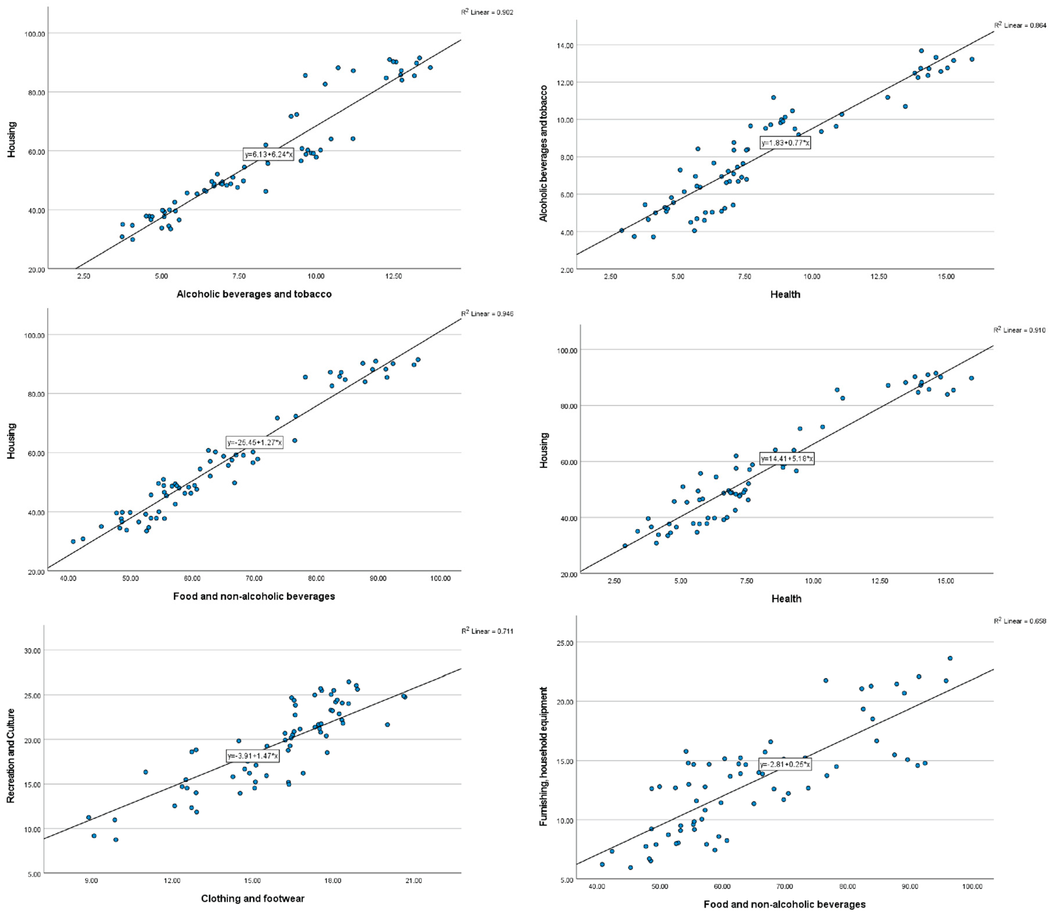
4.3. Estimating Regression Line

The B value refers to the regression coefficient of the model related to household with 0–3 children and the standardized coefficient β is used to compare the influence of each independent variable on the consumption expenditure (see Table 5).
C E t = 2.352   + 0.877 F N A   + 1.552   F A T + 1.149 C F + 1.096 H W E G O + 1.110 F R M + 0.691 H + 1.039   T + 1.078 R C + 1.536 R C H + 1.019 M G S  
Direct interpretation of the results for standardized coefficients:
The p value is statistically significant, which mean that all the variables have a statistically significant impact on the outcome variable (consumption expenditure), except of constant. An unstandardized coefficient slope can be seen whereby the index increases by a value of one for every one unit of change. It is clear that the larger the indexes are, the larger the expenditure is; the goal of this regression analysis is to define the proportion of the individual expenditure depending on a household size (number of children). The standard error value shows the dispersion of expenditures in EUR.
In general, all kinds of expenditure have a significantly positive impact on consumption expenditures (t = 1.423, p < 0.05), so the hypothesis is the following:
H1. 
hypothesis H1 is confirmed.
All examined individual expenses have a significant impact on consumer spending and are influenced by the number of children in the household.
The individual models 0–3 were researched regarding the specific number of children 0–3 in a household, so that individual differences in the interdependence of household expenditure with different number of children are evident. Model U expresses the universal equation of the expenditure structure with respect to all categories of children. Since there is a big difference between the expenditure of households with and without children, individual models were evaluated separately as well as in Table 6.
In all models, the coefficient β4 of the HWEGO value reaches the highest value. The second index with the highest value is the β1 index of the FNA, except for the model with one child, when this index reaches the lowest value (Table 6).
One interesting finding is that in a model with zero and one children, the coefficient of β7 of T (Transport) took the second and third place, while in a model with 3 children (M3) is this expenditure in 9/10 place, which can be caused by the economies of scale.
Coefficient β3 of predictor CF is ranked highest among the models in the M3 model (household with three children), ranked high in M2 model (household with two children) as well, and at the last place in the M1 and M0 models (households with one and zero children). Index β2 of alcohol and tobacco variable is positive in the last places in all models with children. Coefficient β8 of RC (Recreation and culture) is comparatively the highest in M1 and in the M3 it model took the last place compared to other expenditures in the given model.
Coefficient β8 of Rc is, for example, larger than β9 of RCH (restaurants, café, and hotels) in models with zero and 1 children and, on the contrary, in models with two and three children the coefficient β9 is higher than β9.
The coefficient β6 of H-Health is the highest in the order of the M3 model in the last places for the other models. This can be caused by the availability of free health care paid by the public health system (health insurance).
Individual models were evaluated regardless of statistical significance, with the goal of comparison of the share of individual household expenses in terms of household size.
Table 7 also describes the statistical significance of individual coefficients. As it is clear from the data, there are statistically significant coefficients with a value of p > 0.05 for individual models, which are:
-
In the model with one child by coefficients β2 (FAT), β5 z (FRM), and β6 (H);
-
In the model with two children by coefficients β2 (FAT), β3 (CF), and β6 from (H);
-
In the model with three children by coefficients β6 (H), β7 (T), and β8 from (RC).
The results indicate that most (Table 7) individual expenditures under study have a significant impact on consumption expenditures and are influenced by the number of children in a household. Moreover, the R2 = 1.00 depicts that the model explains 100% of the variance in consumption expenditures, with p < 0.05, which confirms the significance of these models.

5. Discussion

In general, it can be concluded based on research and the use of variance analysis that there is a statistically significant difference between household consumption expenditures and the number of children in the household within the scope of the research confirmed by the post hoc multiple comparison as well. This is used for the test of contrasts, the more detailed determination of the differences which groups of households statistically influence these results. Specifically, the data revealed that there is a noteworthy and statistically significant difference in the amount of money spent by households based on the number of individuals in a household. This finding points to the impact of household size on spending patterns (see Figure 3), as larger households tend to spend more on individual goods and services compared to smaller households. Taken together, these results suggest that demographic factors such as the number of household members, including the number of children, play a significant role in shaping household spending behavior and patterns.
Household size can also impact lifestyle factors that affect food expenditure, such as whether the household eats out frequently or prefers to cook at home; this can also influence decisions to use the services of restaurants, cafés, hotels, and recreation and culture services.
The results confirm that there is a significant difference between the household with three and that with less than three children. Larger households may be more likely to cook at home and purchase larger quantities of food, while smaller households may eat out more frequently. In general, this fact influences the cultural and regional factors as well. On the contrary, in other groups, parameters such as consumption expenditure are not all significant in all groups and household sizes in terms of the number of children, as we can see in Table 3.
A special group of expenditure entails health and expenditure on furnishing and household equipment, where there is a significant difference already between zero and any number of children.
The monitoring of the relationship between household size and household expenditure is crucial for many areas to remain vigilant and adaptable, constantly seeking new ways to rank and understand consumer perception behaviors through expenditure. The findings presented in the study point to the significant impact of housing expenditure and the importance of food expenditures in household budgets.
Notably, the coefficient β7 for transportation expenses (T) ranks second and third in models with zero and one child, respectively. However, in the model with three children (M3), transportation expenses fall to the 9th or 10th position. This suggests that economies of scale may play a role in reducing transportation costs as the number of children increases.
The predictor CF, represented by the β3 coefficient, consistently ranks highest in the M3 model (household with three children) and remains high in the M2 model (household with two children) but falls to the lowest position in the M1 and M0 models (households with one and zero children). This indicates that CF has a stronger influence on household expenses in larger families. On the other hand, the β2 index for alcohol and tobacco consistently ranks low in all models with children, suggesting that these expenses are relatively less significant in households with dependents.
Regarding recreation and culture expenses, the coefficient β8 is highest in the M1 model and ranks last in the M3 model compared to other expenditure categories within their respective models. For instance, in models with zero and one child, the coefficient β8 of Rc (recreation and culture) surpasses the coefficient β9 of Rch (restaurants, café, and hotels). However, in models with two and three children, the coefficient β9 is higher than β8. This implies that recreation and culture expenses may take precedence over dining out or hotel stays in smaller families but the trend shifts with an increasing number of children.
The coefficient β6 of H-Health is highest in the M3 model but ranks last in the other models. This discrepancy can be attributed to the availability of free healthcare covered by the public health system, which potentially reduces out-of-pocket health expenses for households with three children.
It is important to acknowledge the limitations of this research. Firstly, the analysis does not account for statistical significance, which may affect the robustness and generalizability of the findings. The omission of statistical tests limits the ability to draw firm conclusions about the significance of the coefficients.
The limitations of this research relate to an extension of this research as well. It is probably not possible to include all parameters and perspectives, which confirm the results of some research conducted on similar subjects in the past. Some studies measure and analyze national income and consumption levels and their changes by understanding the current state of household balances. Most of these models analyze short periods, of one or two years, and mention a need for more effective policy to reduce food insecurity in low-income and lower-middle-income countries (Kim et al. 2022; Kirkpatrick and Tarasuk 2003; Marchetti and Secondi 2017; Russell et al. 2018; Singh and Tiwana 2018; Zezza et al. 2017).
Trinh et al. (2022) draw attention to the importance of the relationship between socioeconomic status and child health. While the relationship between socioeconomic status and child health has been studied extensively in developed countries, evidence is limited for developing countries, using household expenditure as an alternative measure. Our results do not directly address the connection of expenditures and their impact on children’s health; however, this study mentioned above also confirms the validity of including the health care expenditures in our research.
Swathysree et al. (2023) highlight the bias that emerges in the construction of real expenditure overlooking the relative price movements and its consequent implications on for welfare measurements, particularly consumption inequality of rural Indian households during 1999–2012. This model overcomes data limitations like the non-availability of quantity data and item-specific prices.
Raschke (2016) estimates the impact of a given change in the child benefit on food expenditures of households, the probability of owning a home, rent per square meter, and measures of the size of the home as well as parents’ smoking behavior and parents’ alcohol consumption.
Furthermore, the study focuses solely on comparing the share of household expenses based on household size. Other important factors, such as income level, geographical location, and cultural influences are not considered in this analysis. These variables could potentially affect household expenditure patterns and should be taken into account in future research.

6. Conclusions

Consumer perception and behavior are changing and therefore need to be constantly monitored and measured. Confirmation by the current market situation is characterized by dynamism, growing consumer power, and intense competition (Hudak et al. 2017; Madleňák and Madleňáková 2020). In today´s fast-paced and ever-changing marketplace, consumer perception and behavior are subject to constant fluctuations. Businesses need to closely monitor and measure these changes to stay ahead of the curve and remain competitive (Genzorová et al. 2018).
The size of the household is one of the main factors in marketing, business strategies, and policy regulations as well. This means that companies must be attuned to the shifting attitudes and preferences of their audience as well as the broader cultural and economic trends that affect consumer behavior and consider on only the income separately but the factor of the household size as well. Failure to do so can lead to missed opportunities, lost market share, and, ultimately, a decline in overall business performance. In conclusion, household consumption expenditure is a critical measure of economic activity that has significant implications for the economy, marketing, and government policy. Understanding household spending patterns is essential for businesses, policymakers, and economists to make informed decisions about economic growth, marketing strategies, and government policy.
Research in the Slovak Republic has also shown that the expenditure of a household with two children is significantly different from that of a household with three children. The number of children and the type of expenditure significantly influences the difference in expenditure. Families without children have similar expenses as families with one child. Households without and with one child form a separate cluster (confirmed by the international research as well).
Lastly, the study assumes that the coefficients accurately capture the relationships between predictors and household expenses. However, the model specifications and underlying assumptions might introduce potential biases or omitted variables, leading to incomplete or distorted insights. Future research should consider using models that are more sophisticated and a broader range of variables to enhance the understanding of household expenditure dynamics. Household consumption patterns can vary significantly across different demographic groups, regions, and socio-economic classes. The expenditure figure alone does not provide information about the quality of goods and services consumed; all these mentioned above could be a subject of a future research.

Author Contributions

Conceptualization, E.M. and T.C.; methodology, E.M.; validation, E.M. and T.C.; formal analysis, E.M.; investigation, E.M. and T.C.; resources, E.M.; writing—original draft preparation, E.M.; writing—review and editing, T.C.; supervision, T.C.; project administration, T.C.; funding acquisition, T.C. All authors have read and agreed to the published version of the manuscript.

Funding

MŠVVŠ SR funded project VEGA 1/0011/21 Research on the interactions among new emerging technologies, the performance of enterprises and industries based on network technology infrastructure, the application of new business models.

Informed Consent Statement

Not applicable.

Data Availability Statement

The data stated in this study are not publicly available. For further information regarding the data, contact the authors of this article.

Conflicts of Interest

The authors declare no conflict of interest.

References

  1. Anastasiou, Dimitris, Zied Ftiti, Waël Louhichi, and Dimitris Tsouknidis. 2023. Household deposits and consumer sentiment expectations: Evidence from Eurozone. Journal of International Money and Finance 131: 102775. [Google Scholar] [CrossRef]
  2. Armstrong, Richard A. 2014. When to use the Bonferroni correction. Ophthalmic & Physiological Optics: The Journal of the British College of Ophthalmic Opticians (Optometrists) 34: 502–8. [Google Scholar] [CrossRef]
  3. Armstrong, Richard A., Frank Eperjesi, and Bernard Gilmartin. 2002. The application of analysis of variance (ANOVA) to different experimental designs in optometry. Ophthalmic and Physiological Optics 22: 248–56. [Google Scholar] [CrossRef] [PubMed]
  4. Armstrong, Richard A., Sarah V. Slade, and Frank Eperjesi. 2000. An introduction to analysis of variance (ANOVA) with special reference to data from clinical experiments in optometry. Ophthalmic & Physiological Optics: The Journal of the British College of Ophthalmic Opticians (Optometrists) 20: 235–41. [Google Scholar] [PubMed]
  5. Attanasio, Orazio P., and Valérie Lechene. 2014. Efficient Responses to Targeted Cash Transfers. Journal of Political Economy 122: 178–222. [Google Scholar] [CrossRef]
  6. Banks, James, Richard Blundell, and Arthur Lewbel. 1997. Quadratic Engel Curves and Consumer Demand. The Review of Economics and Statistics 79: 527–39. [Google Scholar] [CrossRef]
  7. Belete, Abenet, Chris O. Igodan, C M’Marete, and Wim van Averbeke. 1999. Analysis Of Rural Household Consumption Expenditure In South Africa: The Case Of Food Plot Holders In Tyefu Irrigation Scheme In The Eastern Cape Province/Analise Van Verbruiksbesteding Van Landelike Huishoudings In Suid-Afrika: ’N Gevallestudie Van Kleinboere In Tyefu Besproeiingskema In Die Ooskaap Provinsie. Agrekon 38: 194–203. [Google Scholar] [CrossRef]
  8. Binder, Carola. 2020. Coronavirus Fears and Macroeconomic Expectations. The Review of Economics and Statistics 102: 721–30. [Google Scholar] [CrossRef]
  9. Browning, Martin, and Thomas F. Crossley. 2001. The Life-Cycle Model of Consumption and Saving. Journal of Economic Perspectives 15: 3–22. [Google Scholar] [CrossRef]
  10. Bui, Dzung, Lena Dräger, Bernd Hayo, and Giang Nghiem. 2023. Macroeconomic expectations and consumer sentiment during the COVID-19 pandemic: The role of others’ beliefs. European Journal of Political Economy 77: 102295. [Google Scholar] [CrossRef]
  11. Chai, Andreas, and Alessio Moneta. 2010. Retrospectives: Engel Curves. Journal of Economic Perspectives 24: 225–40. [Google Scholar] [CrossRef]
  12. DATAcube. 2023. Available online: https://slovak.statistics.sk/wps/portal/ext/Databases/DATAcube_sk/!ut/p/z1/jY_LDoIwEEW_hS_oLeW5HFBKDUEK8rAbw8qQKLowfr8NcStyd5M5506GGTYwM4_v6Tq-psc83ux8NsGFtNZN0XWQnZtBCS5Rti2QhaxfAB2qKEk4ISrrPdSJKlkfPA7PZ8aus6ZyKfZkuquP1j-lbtQUgQvwr78CmC33U0m5FxZAVEgfivK2jrUQILHNx48QtvkrgFmv75lZkLUP_nU8763NgIkc5wNzscHm/dz/d5/L2dJQSEvUUt3QS80TmxFL1o2X1ZMUDhCQjFBME9RUDYwQUlLTjRTOUkwMlMz/ (accessed on 8 January 2023).
  13. De Vreyer, Philippe, Sylvie Lambert, and Martin Ravallion. 2020. Unpacking Household Engel Curves. Cambridge, MA: National Bureau of Economic Research. [Google Scholar] [CrossRef]
  14. Easaw, Joshy Z., and Atanu Ghoshray. 2007. Confidence or competence: Do presidencies matter for households’ subjective preferences? European Journal of Political Economy 23: 1025–37. [Google Scholar] [CrossRef]
  15. Enger, Ernst. 1985. Lebenskoten Belgischer Arbeiter-Familien Fruher and jetz. Statistical Institute Bulletin 9: 1–74. [Google Scholar]
  16. Eurostat. 2023. Available online: https://ec.europa.eu/eurostat/web/main/search/-/search/estatsearchportlet_WAR_estatsearchportlet_INSTANCE_bHVzuvn1SZ8J?p_auth=FZrMZWYF&text=household+composition&_estatsearchportlet_WAR_estatsearchportlet_INSTANCE_bHVzuvn1SZ8J_collection=&_estatsearchportlet_WAR_estatsearchportlet_INSTANCE_bHVzuvn1SZ8J_theme= (accessed on 8 January 2023).
  17. Genzorová, Tatiana, Tatiana Corejova, and Natália Stalmašeková. 2018. Comparing The Use Of Digital Platforms In Tourism. CBU International Conference Proceedings 6: 152–55. [Google Scholar] [CrossRef]
  18. Huang, Yanyan, and Fuzhong Chen. 2022. The Impact of Household Debt on Food Expenditure and Its Mechanism in Urban China. Journal of Family and Economic Issues 43: 466–75. [Google Scholar] [CrossRef]
  19. Hudak, Martin, Radovan Madlenak, and Veronika Brezaniova. 2017. The Impact of Advertisement on Consumer´s Perception. CBU International Conference Proceedings 5: 187–91. [Google Scholar] [CrossRef]
  20. Jacobson, David, Petroula M. Mavrikiou, and Christos Minas. 2010. Household size, income and expenditure on food: The case of Cyprus. The Journal of Socio-Economics 39: 319–28. [Google Scholar] [CrossRef]
  21. Jayasinghe, Maneka, and Christine Smith. 2021. Poverty Implications of Household Headship and Food Consumption Economies of Scales: A Case Study from Sri Lanka. Social Indicators Research 155: 157–85. [Google Scholar] [CrossRef]
  22. Kandil, Siham. 2020. Food Expenditure Patterns In Rural And Urban Areas In Egypt (In Arabic). Journal of Productivity and Development 25: 195–212. [Google Scholar] [CrossRef]
  23. Kim, Sihyeon, Byeongchan Seong, Young-Geun Choi, and In-kwon Yeo. 2022. A study on time series linkage in the Household Income and Expenditure Survey. Korean Journal of Applied Statistics 35: 553–68. [Google Scholar] [CrossRef]
  24. Kirkpatrick, Sharon, and Valerie Tarasuk. 2003. The relationship between low income and household food expenditure patterns in Canada. Public Health Nutrition 6: 589–97. [Google Scholar] [CrossRef] [PubMed]
  25. Leser, Conrad Emanuel Victor. 1963. Forms of Engel Functions. Econometrica 31: 694–703. [Google Scholar] [CrossRef]
  26. Logan, Trevon D. 2011. Economies of Scale in the Household: Puzzles and Patterns from the American Past. Economic Inquiry 49: 1008–28. [Google Scholar] [CrossRef]
  27. Ludvigson, Sydney C. 2004. Consumer Confidence and Consumer Spending. Journal of Economic Perspectives 18: 29–50. [Google Scholar] [CrossRef]
  28. Madleňák, Radovan, and Lucia Madleňáková. 2020. Multi-Criteria Evaluation of E-Shop Methods of Delivery from the Customer’s Perspective. Transport Problems 15: 5–14. [Google Scholar] [CrossRef]
  29. Marchetti, Stefano, and Luca Secondi. 2017. Estimates of Household Consumption Expenditure at Provincial Level in Italy by Using Small Area Estimation Methods: “Real” Comparisons Using Purchasing Power Parities. Social Indicators Research 131: 215–34. [Google Scholar] [CrossRef]
  30. Mulamba, Kabeya Clement. 2022. Relationship between households’ share of food expenditure and income across South African districts: A multilevel regression analysis. Humanities and Social Sciences Communications 9: 428. [Google Scholar] [CrossRef]
  31. Murray, Alan P. 1964. Wage-Withholding And State Income Taxes. National Tax Journal 17: 403–17. [Google Scholar] [CrossRef]
  32. Donkoh, Samuel A., Hamdiyah Alhassan, and Paul K. Nkegbe. 2014. Food expenditure and household welfare in Ghana. African Journal of Food Science 8: 164–75. [Google Scholar] [CrossRef]
  33. Pitas, Nick, and Sharon Zou. 2023. Consumer Confidence and Recreation Behavior: Willingness to Buy and Attitudes toward a Proposed Recreation User Fee Increase. In Society & Natural Resources. Online: Taylor & Francis, pp. 1–16. [Google Scholar] [CrossRef]
  34. Raschke, Christian. 2016. The Impact of the German Child Benefit on Household Expenditures and Consumption. German Economic Review 17: 438–77. [Google Scholar] [CrossRef]
  35. Russell, Joanna, Anne Lechner, Quentin Hanich, Aurélie Delisle, Brooke Campbell, and Karen Charlton. 2018. Assessing food security using household consumption expenditure surveys (HCES): A scoping literature review. Public Health Nutrition 21: 2200–10. [Google Scholar] [CrossRef] [PubMed]
  36. Singh, Taranjeet, and Balwinder Singh Tiwana. 2018. Distribution Pattern of Consumption Expenditure of Loan Waiver Beneficiary Households in Punjab. Indian Journal of Economics and Development 14: 650. [Google Scholar] [CrossRef]
  37. Su, Chi Wie, Fangying Liu, Meng Qin, and Tsangyao Chnag. 2023a. Is a consumer loan a catalyst for confidence? Economic Research-Ekonomska Istraživanja 36: 2142260. [Google Scholar] [CrossRef]
  38. Su, Chi Wei, Muhammad Umar, and Tsangyao Chang. 2023b. How consumer confidence is reshaping the outbound tourism expenditure in China? A lesson for strategy makers! Economic Research-Ekonomska Istraživanja 36: 2106266. [Google Scholar] [CrossRef]
  39. Swathysree, S S, Manisha Chakrabarty, and Debopriti Bhattacharya. 2023. Getting Real in the Real Consumption Expenditure: A Case of Rural India. Journal of Quantitative Economics 21: 817–46. [Google Scholar] [CrossRef]
  40. Trinh, Trong-Anh, Preety Srivastava, and Sarah Brown. 2022. Household expenditure and child health in Vietnam: Analysis of longitudinal data. Journal of Demographic Economics 88: 351–77. [Google Scholar] [CrossRef]
  41. Umeh, Joseph C., and Benjamin C. Asogwa. 2012. Determinants of Farm Household Food Expenditure: Implications for Food Security in Rural Nigeria. Paper presented at International Conference on Ecology, Agriculture and Chemical Engineering, Phuket, Thailand, December 18–19. [Google Scholar]
  42. Working, Holbrook. 1943. Statistical Laws of Family Expenditure. Journal of the American Statistical Association 38: 43–56. [Google Scholar] [CrossRef]
  43. Zezza, Alberto, Calogero Carletto, John L. Fiedler, Pietro Gennari, and Dean Jolliffe. 2017. Food counts. Measuring food consumption and expenditures in household consumption and expenditure surveys (HCES). Introduction to the special issue. Food Policy 72: 1–6. [Google Scholar] [CrossRef]
  44. Zhang, Zihan. 2023. Check and Balance Overspending in Average American Household Consumption. Highlights in Business, Economics and Management 7: 1–7. [Google Scholar] [CrossRef]
Figure 1. Consumption expenditure according to the household size (children) 1994–2021.
Economies 12 00009 g001
Figure 2. Linear regression lines of selected combinations of consumption expenditures.
Economies 12 00009 g002
Figure 3. Bonferroni post hoc comparison results.
Economies 12 00009 g003
Table 1. ANOVA and measures of association in the Slovak Republic.
FEta SquaredSig.
Household Consumption ExpenditureF (3,64) = 66,021η2 = 0.7560.000
Food and non-alcoholic beverages F (3,64) = 146,302η2 = 0.8730.000
Alcoholic beverages and tobacco F (3,64) = 142,051η2 = 0.8690.000
Clothing and footwear F (3,64) = 20,457η2 = 0.4900.000
Housing, water, electricity, gas, and other fuels F (3,64) = 417,786η2 = 0.9510.000
Furnishings, household equipment, and routine maintenance of the house F (3,64) = 23,419η2 = 0.5230.000
Health F (3,64) = 109,748η2 = 0.8370.000
Transport F (3,64) = 5611η2 = 0.2080.002
Recreation and Culture F (3,64) = 25,922η2 = 0.5490.000
Restaurants, café, and hotels F (3,64) = 6760η2 = 0.2410.000
Miscellaneous goods and services F (3,64) = 19,844η2 = 0.4820.000
Table 2. Post hoc Bonferroni Multiple Comparison A.
ExpenditureHousehold Size (Children)Mean DifferenceSig.
Household consumption expenditure
Food and non-alcoholic beverages
Alcoholic beverages and tobacco
Housing, water, electricity, gas, and other fuels
0
1
2
3
YES0.000
Table 3. Post hoc Bonferroni multiple comparison B.
Dependent VariableHousehold Size (Children)Different from Each OtherMean DifferenceSig.
Zscore: Clothing and footwear01−0.256795831.000
20.352378490.989
3sig.0.000
120.609174320.108
3sig.0.000
23sig.0.000
30, 1, 2sig.0.000
Zscore: Furnishings, household equipment, and routine maintenance of the house01, 2, 3sig.0.000
10, 3sig.0.001
20.629215560.070
230.307226361.000
30, 1sig.0.000
2−0.307226371.000
Zscore: Health01, 2, 3sig.0.000
10, 2, 3sig.0.000
230.348241080.100
30, 1sig.0.000
2−0.348241080.100
Zscore: Transport01−0.297693961.000
20.305577101.000
3sig.0.026
120.603271050.347
3sig.0.001
230.619939990.308
30, 1sig.0.026
2−0.619939990.308
Zscore: Recreation and culture010.345805940.884
2, 30.706463240.023
120.360657290.786
3sig.0.000
23sig.0.000
30, 1, 2sig.0.000
Zscore: Restaurants, café, and hotels01−0.553627580.450
2−0.209458511.000
30.773271520.084
120.344169071.000
3sig.0.000
23−0.982730020.012
30−0.773271520.084
1sig.0.000
2−0.982730020.012
Zscore: Miscellaneous goods and services01−0.315094501.000
20.462110080.432
13sig.0.000
2, 30.777204580.018
231.044612560.018
30, 1, 2sig.0.000
Table 4. Consumption expenditure correlations.
Consumption ExpenditureEstimate (R)R2
Housing (water, electricity, gas, and other fuels)<-->Restaurants, café, and hotels0.3430.117649
Housing (water, electricity, gas, and other fuels)<-->Transport0.4130.170569
Health<-->Restaurants, café, and hotels0.4270.182329
Recreation and Culture<-->Miscellaneous goods and services0.4310.185761
Food and non-alcoholic beverages<-->Transport0.4500.2025
Food and non-alcoholic beverages<-->Restaurants, café, and hotels0.4610.212521
Health<-->Transport0.4970.247009
Health<-->Miscellaneous goods and services0.5090.259081
Alcoholic beverages and tobacco<-->Restaurants, café, and hotels0.5180.268324
Alcoholic beverages and tobacco<-->Transport0.5230.273529
Clothing and footwear<-->Miscellaneous goods and services0.5380.289444
Clothing and footwear<-->Health0.5430.294849
Transport<-->Recreation and culture0.5530.305809
Housing (water, electricity, gas, and other fuels)<-->Miscellaneous goods and services0.5540.306916
Furnishing, household equipment, etc.<-->Restaurants, café, and hotels0.5570.310249
Clothing and footwear<-->Housing (water, electricity, gas, and other fuels)0.5680.322624
Furnishing, household equipment, etc.<-->Recreation and culture0.5750.330625
Food and non-alcoholic beverages<-->Clothing and footwear0.5750.330625
Clothing and footwear<-->Furnishing, household equipment0.5870.344569
Food and non-alcoholic beverages<-->Miscellaneous goods and services0.6010.361201
Recreation and culture<-->Restaurants, café, and hotels0.6210.385641
Alcoholic beverages and tobacco<-->Clothing and footwear0.6410.410881
Alcoholic beverages and tobacco<-->Miscellaneous goods and services0.6550.429025
Clothing and footwear<-->Restaurants, café, and hotels0.6600.4356
Clothing and footwear<-->Transport0.6720.451584
Health<-->Recreation and culture0.7000.49
Transport<-->Miscellaneous goods and services0.7040.495616
Housing (water, electricity, gas, and other fuels)<-->Recreation and culture0.7060.498436
Food and non-alcoholic beverages<-->Recreation and culture0.7120.506944
Restaurants, café, and hotels<-->Miscellaneous goods and services0.7200.5184
Furnishing, household equipment, etc.<-->Transport0.7240.524176
Transport<-->Restaurants, café, and hotels0.7490.561001
Alcoholic beverages and tobacco<-->Recreation and culture0.7530.567009
Furnishing, household equipment, etc.<-->Miscellaneous goods and services0.7620.580644
Alcoholic beverages and tobacco<-->Furnishing, household equipment, etc.0.7720.595984
Housing (water, electricity, gas, and other fuels)<-->Furnishing, household equipment, etc.0.7930.628849
Furnishing, household equipment, etc.<-->Health0.8040.646416
Food and non-alcoholic beverages<-->Furnishing, household equipment, etc.0.8110.657721
Clothing and footwear<-->Recreation and culture0.8550.731025
Alcoholic beverages and tobacco<-->Health0.9300.8649
Alcoholic beverages and tobacco<-->Housing (water, electricity, gas, and other fuels)0.9500.9025
Food and non-alcoholic beverages<-->Alcoholic beverages and tobacco0.9540.910116
Housing (water, electricity, gas, and other fuels)<-->Health0.9540.910116
Food and non-alcoholic beverages<-->Health0.9650.931225
Food and non-alcoholic beverages<-->Housing (water, electricity, gas, and other fuels)0.9730.946729
Table 5. t-test for regression coefficients of the consumption expenditure by household size.
Model U
(0–3 Children)
Unstandardized CoefficientsStandardized CoefficientstSig.
BStd. Errorβ
β02.3521.653 1.4230.160
β10.8770.0650.20213.4250.000
β21.5520.2360.0716.5770.000
β31.1490.1200.0499.5870.000
β41.0960.0580.32918.9460.000
β51.1100.0970.07811.4750.000
β60.6910.2590.0382.6630.010
β71.0390.0380.16127.6330.000
β81.0780.0870.07812.3180.000
β91.5360.1120.08713.6880.000
β101.0190.0810.08912.5700.000
Table 6. Unstandardized coefficients of research models.
ModelUnstandardized Coefficientsβ0β1β2β3β4β5β6β7β8β9β10
M0
(Zero children)
B−0.1070.200.0910.0580.3580.0680.0610.1630.0680.0510.104
Std. Error0.0530.020.0260.0130.0270.0140.0230.0160.0240.0270.019
M1
(One children)
B8.0430.5302.7331.8040.9031.5131.5211.0500.9351.4640.952
Std. Error9.9040.2061.3890.5730.3430.6650.7600.0730.3940.5650.288
M2
(Two children)
B0.0290.2190.0500.0590.3570.1040.0580.1390.0690.0800.075
Std. Error0.0830.0700.0500.0260.0890.0300.0590.0270.0300.0360.030
M3
(Three children)
B0.0730.1880.0010.1030.4220.1500.1660.0440.0390.0900.055
Std. Error0.1110.0720.0510.0310.0730.0550.0850.0600.0250.0400.049
Table 7. Statistical significance of individual coefficients β0–β10.
ModelStandardized Coefficientsβ0β1β2β3β4β5β6β7β8β9β10
0Beta 0.1510.0790.0740.1810.0920.0550.2890.0920.0920.152
t−2.0108.0243.4614.34112,8694.8232.5679.8822.7451.8725.345
sig.0.0910.0000.0130.0050.0000.0030.0430.0000.0340.0110.002
1Beta 0.0930.1040.0870.1170.1340.0680.2890.0950.1670.142
t0.8122.5651.9683.1462.6292.2762.002144402.3742.5933.306
Sig.0.0450.0430.0970.0200.0390.0630.0920.0000.0450.0410.016
2Beta 0.1550.0310.0750.1480.1670.0430.2500.0890.1410.110
t0.3493.1261.0002.2734.0063.4330.9875.2162.3322.2342.535
Sig.0.7390.0200.3560.0630.0070.0140.3620.0020.0480.0470.044
3Beta 0.1240.0000.2090.1610.2100.1250.0830.0550.1250.061
t0.6612.6010.0233.2605.7902.7201.9470.7321.5872.2191.120
Sig.0.5330.0410.9830.0170.0010.0350.0990.4920.1640.0480.031
Disclaimer/Publisher’s Note: The statements, opinions and data contained in all publications are solely those of the individual author(s) and contributor(s) and not of MDPI and/or the editor(s). MDPI and/or the editor(s) disclaim responsibility for any injury to people or property resulting from any ideas, methods, instructions or products referred to in the content.

