A Novel Ensemble Machine Learning Approach for Bioarchaeological Sex Prediction

Abstract

I present a novel machine learning approach to predict sex in the bioarchaeological record. Eighteen cranial interlandmark distances and five maxillary dental metric distances were recorded from n = 420 human skeletons from the necropolises at Alfedena (600–400 BCE) and Campovalano (750–200 BCE and 9–11th Centuries CE) in central Italy. A generalized low rank model (GLRM) was used to impute missing data and Area under the Curve—Receiver Operating Characteristic (AUC-ROC) with 20-fold stratified cross-validation was used to evaluate predictive performance of eight machine learning algorithms on different subsets of the data. Additional perspectives such as this one show strong potential for sex prediction in bioarchaeological and forensic anthropological contexts. Furthermore, GLRMs have the potential to handle missing data in ways previously unexplored in the discipline. Although results of this study look promising (highest AUC-ROC = 0.9722 for predicting binary male/female sex), the main limitation is that the sexes of the individuals included were not known but were estimated using standard macroscopic bioarchaeological methods. However, future research should apply this machine learning approach to known-sex reference samples in order to better understand its value, along with the more general contributions that machine learning can make to the reconstruction of past human lifeways.

1. Introduction

Accurate sex prediction of archaeological skeletal remains is a fundamental step for reconstructing biological and demographic profiles of past humans. After an archaeological site is surveyed and excavated and unknown human remains are identified, documented, and recovered, the sex and age of deceased individuals are commonly estimated using macroscopic methods of the pelvis, skull, and teeth [1,2,3]. However, because female and male biological maturation rates differ [4,5], sex misidentification can lead to data recording bias and depreciated interpretability. After sex has been macroscopically estimated and with the assistance of other biological and archaeological contextual information, the identities and lifeways of the deceased can be reconstructed in bioarchaeological contexts. However, traditional macroscopic sex estimation methods possess varying degrees of accuracy [6,7,8,9,10,11]. For example, the pelvis and cranium might provide conflicting sex estimation results even within the same individual. This process is further complicated by other aspects, particularly of age, as tooth crown calcification and eruption and bone epiphyseal fusion are useful until early adulthood when 3rd molars erupt and bony ossification centers fuse skeletal elements into their final, united shapes. Pelvic, cranial suture, and sternal rib end methods are used to predict age in individuals through later stages of adulthood, albeit with wider margins of error.

Craniometric dimensions are frequently used as proxies for genetic relatedness of past humans due to their potentially heritable nature and correlations with neutral and adaptive genetic variation and selection [12,13,14,15,16,17,18,19,20]. In the absence of genetic information, these methods are used to approximate the genetic and evolutionary relationships of past humans [21], thus making accurate sex classification an integral first step in the reconstruction of other biological and demographic parameters. Hence, further examinations of sex correlations with other lines of evidence such as burial location, material culture, musculoskeletal stress markers, health, diet, disease, trauma prevalence, and biological relatedness will be skewed if sex is first misclassified.

Machine learning is slowly gaining a foothold in bioarchaeology and forensic anthropology despite our discipline’s deep ties to statistics and computational research for investigation of large quantitative datasets. Cunningham’s [22] pioneering machine learning social anthropological work for rule-based kinship structure detection set a high bar for anthropologists of all subdisciplines to aspire. However, her work remains largely unrecognized even though it exemplifies the types of problem-and-dataset-driven questions faced by bioarchaeologists. This discrepancy persists despite the promise for bioarchaeological machine learning applications for predicting sex, age, ancestry, body mass, and stature in forensic anthropology, radiography, and anatomy [23,24,25,26,27,28,29,30,31]. Even less bioarchaeological research has focused on missing data imputation [32].

Therefore, more examples are needed to better contextualize our methodological understandings of sex estimation techniques. This research is an extension of Muzzall et al. (2017) [33], which improved sex prediction accuracy of the William W. Howells Worldwide Craniometric Dataset and provided another example of the strong potential for machine learning to assist in sex prediction in bioarchaeological contexts. Here, I use a generalized low rank model to impute large amounts of missing data for a stratified cross-validated supervised ensemble machine learning approach. This framework consists of eight algorithms total and is fit to cranial interlandmark and dental metric distances to predict binary sex from six pelvic and cranially estimated samples at Alfedena (600–400 BCE) and Campovalano (750–200 BCE and 9–11th Centuries CE) in central Italy.

Italy is home to one of the most colossal bioarchaeological contexts on Earth and represents humans’ deep history throughout the region. Its central Mediterranean location, deep temporal breadth, and geological and environmental diversities have been influential in shaping the genetic, morphological, and cultural histories of the region [34,35,36,37,38,39]. Humans here developed some of the richest and most divergent forms of social interaction through worship, architecture, iconography and writing, and empires that persisted for long periods of time and across the globe via trade, warfare, and colonization. Central Italy was a particular crossroads between Africa and Europe and the Near East and Iberia and was home to many chiefdoms and nation-states that contained both shared and varied forms of settlement patterns, social and burial organization, material cultures, mortuary behaviors, and skeletal-dental morphologies. As a result, Italy’s bioarchaeological record provides a space to experiment with new methodologies for sex prediction.

2. Materials and Methods

2.1. Dataset

The dataset consists of metric cranial and dental data from n = 240 males and n = 180 females from central Italy: four locations from the Iron Age necropolis at Alfedena (600–400 BCE), the Iron Age graveyard at Campovalano (750–200 BCE), and the Medieval cemetery at Campovalano (9–11th Centuries CE) (

Table 1. Location, time period, and sex distributions for males and females from Central Italy used in this study.

Location	Time Period	Male	Female
Alfedena Arboreto	600–400 BCE	9	10
Alfedena Campo Consolino	600–400 BCE	61	19
Alfedena Scavi Mariani	600–400 BCE	37	28
Alfedena Sergi Museum	600–400 BCE	19	13
Campovalano Iron Age	750–200 BCE	89	77
Campovalano St. Peter	9–11th C. CE	25	33
Total		240	180

). The ground truth sexes of these individuals were not known due to their antiquity and were estimated using standard macroscopic methods found in [1] by the original archaeologists [40,41] and by the author.

Cranial metric data were collected from twelve standard anatomical landmarks: four from the face, four from the cranial vault, and four from the cranial base (

Table 2. Cranial anatomical landmarks used in this study. The four landmarks from each of the three regions produced eighteen total interlandmark distances—six for each region [1 (and references therein)].

Face	Definition
Nasion (n)	The intersection of the naso-frontal suture in the midsagittal plane
Prosthion (pr)	The location of the anteriorly located portion of the anterior surface of the alveolar process at the most anterior point of the alveolar process
Right frontomalare	The location where the zygomaticofrontal suture intersects the orbital margin
orbitale (fmorR)
Left zygomaxillare (zymL)	The most inferior and anterior location on the zygomaticomaxillary suture
Vault
Bregma (b)	The landmark where the sagittal and coronal sutures meet in the midsagittal plane. In cases where the sagittal suture deflects laterally, an estimation must be made of the location in the midsagittal plane
Lambda (l)	The landmark where the left and right lambdoidal sutures intersect the sagittal suture. The landmark must be estimated when the suture intersection is obliterated, or where strongly serrated sutures are present
Right Asterion (astR)	The juncture of the lambdoid, parietomastoid, and occipitomastoid sutures
Left Frontotemporale	The most medial and anterior point on the superior temporal line on the frontal bone
(ftL)
Base
Nasion (n)	The intersection of the naso-frontal suture in the midsagittal plane
Basion (ba)	The inner border where the anterior portion of the foramen magnum is intersected by the midsagittal plane
Hormion (h)	The juncture of the sphenoid and vomer bones in the midsagittal plane
Left Porion (poL)	The most superior point on the external margin of the external auditory meatus

). This produced a total of eighteen cranial interlandmark distances, six from each of the four landmarks from the three cranial regions.

Dental metric data consisted of maximum mesiodistal dimensions of the right (or left-substituted when the right antimere was missing) maxillary canine (XC) and buccolingual breadths of the right mesial (P3) and distal (P4) premolars and first (M1) and second (M2) molars [42]. Thus, six different subsets of the data were used: (1) six metrics from the face, (2) six from the vault, (3) six from the base, (4) eighteen from the cranium (the combined face, vault, and base metrics), (5) five from the dentition, and (6) twenty-three from the total combined cranial and dental data. Tukey boxplots are used to illustrate sex differences in these metrics.

2.2. Missing Data

Missing data were prevalent from all areas of measurement and proportions of missing values for the face, vault, base, and dentition are shown in

Table 3. Percentage of missing data for each variable.

Bony Region	Measurement	Proportion Missing Male	Proportion Missing Female
Face	n_pr	63	67
	n_fmorR	54	58
	n_zymL	57	65
	pr_fmorR	63	68
	pr_zymL	63	69
	fmorR_zymL	63	71
Vault	b_l	38	47
	b_astR	38	46
	b_ftL	42	51
	l_astR	37	44
	l_ftL	44	54
	astR_ftL	46	54
Base	n_ba	61	66
	n_h	63	68
	n_poL	53	61
	ba_h	65	69
	ba_poL	57	62
	h_poL	61	66
Dentition	XC	59	69
	P3	53	63
	P4	50	66
	M1	49	46
	M2	53	53

. A generalized low rank model (GLRM) was used to impute the missing values. GLRMs function as an extension of principal component analysis (PCA) for low rank matrix tabular dataset approximation, by

“approximating a data set as a product of two low dimensional factors by minimizing an objective function. The objective will consist of a loss function on the approximation error together with regularization of the low dimensional factors. With these extensions of PCA, the resulting low rank representation of the data set still produces a low dimensional embedding of the data set, as in PCA”

[43] (p. 3)

A generalized low rank model is essentially an unsupervised approach for data completion that uses clustering of known data in reduced dimensional space. The advantage of this data-adaptive approach to reconstruct missingness in the skeletal and dental remains instead of column mean, median, or k-nearest neighbor imputation is that it effectively uses clustering of features to impute the missing data, which makes sense given that the missingness of the data arises directly from missingness in the skeletal remains themselves. Missingness indicators were also added as columns to the dataset to indicate exactly where missing and imputed data were located. These columns also functioned as predictor variables in the machine learning models to see if the location of missing data was related to sex prediction ability.

2.3. Ensemble Machine Learning

Machine learning is defined as “a vast set tools for understanding data” [44] (p. 1). It originated as a combination of computer science and statistics, but its greatest strength is its breadth of research application [45,46]. Early examples stem from the social and cognitive sciences that attempted to predict and imitate human behavior [47,48,49]. In this research I use a supervised classification machine learning approach because the goal is to predict a categorical outcome (predict male sex from binary male/female options) using the craniodental features as predictor variables.

Ensembles are useful supervised machine learning methods because they optimize predictor accuracy through combinations of a suite of less accurate models [50]. They are preferred to fitting single algorithms for prediction because classification performance of single algorithms might differ due to variance (sensitivity to differences in the training data), algorithmic bias (erroneous assumptions about the relationships between the selected algorithm and the data), and/or algorithmic hyperparameter settings (pre-defined options that are selected before model training). The SuperLearner approach [51,52] is an algorithm that uses cross-validation [53] to estimate the performance of several machine learning models, and/or the same algorithm(s) with different hyperparameter settings. It then produces an optimal weighted average of those models (an “ensemble model”), using external cross-validation. This method is as accurate asymptotically as any single best-performing algorithm. I fit the eight algorithms (five constituent algorithms, the weighted SuperLearner ensemble, the benchmark mean of the Y outcome variable, and the resulting “DiscreteSL” single best performing algorithm/combination of algorithms) to predict binary sex classification for each of the six subsets of the data described above as the predictors: the face, vault, base, combined cranial regions, dentition, and combined craniodental data. In this sense, SuperLearner is essentially stacked/blended learning where the SuperLearner ensemble algorithm provides the ideal combinations of base learners by utilizing weighted combinations to provide asymptotically optimal learner configurations across algorithms and different subsets of the data.

Besides the SuperLearner approach, there are other ways to utilize machine learning ensembles. For example, the random forest algorithm is in itself an ensemble—it is “random” because it is based on individual bootstrap-aggregated (a sampling with replacement model averaging technique for variance reduction) decision trees and also because each individual tree uses a subset of predictor variables at each decision split (instead of using all predictors like a regular decision tree does); it is a “forest” because many trees are grown. The predictions based on each of these trees in the forest is then applied to the out-of-bag samples—holdout data not included in the training process of each tree—to evaluate performance and provide error estimates. The outcome variable is then predicted based on the majority vote of class labels for all the trees in the case of classification, or the prediction average across all trees in the case of regression. Bagging and boosting can be used to improve the performance of a variety of other algorithms as well. The eight different algorithms used in this study are defined in

Table 4. Definitions of the eight machine learning algorithms used in this research.

Algorithm	Description	Reference
Logistic regression	Logistic regression models the relationships between the outcome variable (male/female sex) and the predictor variables. It computes the probability that the Y variable (sex) belongs to one of the two binary classes.	Dobson, 1990 [54]
Lasso	Lasso (least absolute shrinkage and selection operator) is a form of penalized regression (L1) that produces a sparse solution to remove predictor variables from the model that are not related to the outcome.	Friedman et al.,. 2010 [55]
Decision tree	A decision tree is a relatively simple tree-based method that gauges the probability of classifying the outcome based on the predictor variables before splitting a given decision node a certain number of times until there are no longer enough observations to split.	Breiman et al., 1984 [56]
Ranger (random forest)	Ranger is a decorrelated random forest ensemble classifier method that uses the average of multiple bootstrapped decision tree models for classification. Unlike single decision tree models that use all predictors at each split, random forests use only a random subsample of the total predictors for each split in each tree.	Breiman, 2001 [57]; Wright and Ziegler, 2017 [58]
Xgboost	A gradient boosted tree is another tree-based method that fits a tree to the residuals of the previous tree in succession. It downweights easily predicted cases but upweights those that it cannot predict. This continues over many iterations so that weak trees are “boosted” into strong ones.	Freund and Schapire, 1999 [59]; Chen et al.,. 2019 [60]
SuperLearner	The SuperLearner algorithm is an optimal weighted ensemble average that improves predictor construction and is flexible in that it can perform well on different data distributions and protects against overfitting through external cross-validation. Individual algorithm weights can be investigated to see which ones contribute most to the ensemble.	van der Laan et al., 2007 [51]; Kennedy, 2017 [61]
Mean of Y	The mean of Y (dependent variable) is the benchmark algorithm based only on the mean. This is a very simple prediction so the more complex algorithms should perform better than this one. It should not be the best single-performing algorithm and should have a low weight in the weighted-average ensemble. If it is the best performing algorithm something is likely wrong.	Polley and van der Laan, 2010 [52]
DiscreteSL	The discrete SuperLearner is the single best performing algorithm(s) as identified by the SuperLearner. Alternatively, this might also correspond to the combination of best performing algorithms at different cross-validation folds, in which case the DiscreteSL AUC-ROC will not be identical to that of a single algorithm.	Polley and van der Laan, 2010 [52]

.

2.4. Evaluating Model Performance

Stratified 20-fold cross-validated Area Under the Curve—Receiver Operating Characteristic (AUC-ROC) was used to evaluate the performance of the individual algorithms while an external/nested 20-fold cross-validation layer was used to estimate performance on the blended SuperLearner ensemble model via a separate holdout sample [61,62].

Stratified k-fold cross-validation is a process that divides the data into equally sized portions and trains a model on k-1 portions of the data so that the model can learn the relationship between male/female sex outcomes and the various craniodental predictor variables. The one holdout portion is used for testing purposes (but not for fitting the SuperLearner) and this process is repeated k times. I chose 20 folds, so each algorithm was trained on 19 portions of the data (95%) and tested on the one holdout (5%). This process was repeated twenty times, with the holdout set rotated each time. This process allows every data point to be in the test set once. This also produces standard errors for the performance of each algorithm that can be compared to the SuperLearner average.

The receiver operator characteristic curve itself represents the probability that a binary outcome (male or female predicted sex, in this case) is correctly classified [63] while the AUC-ROC provides the degree of separability for the sexes that the model achieves. The receiver operator characteristic curve models the sensitivity (true positive rate) versus specificity (true negative rate) at various thresholds along the receiver operator characteristic curve. Maximization of AUC-ROC is ideal, which ranges from zero (no predictive ability) to 0.5 (equivalent to random guessing) to 1.0 (perfect prediction). AUC-ROC is more useful for prediction of imbalanced classes and to prevent overfitting of a single class compared to simple classification accuracy.

Instead of fitting the models separately and looking at the performance (lowest risk), algorithms should be fit simultaneously. Risk is the average loss function used here and measures how far off the prediction was for a given observation and is calculated by nonnegative least squares error; the lower the risk the fewer errors were made by the model. SuperLearner also identifies which single algorithm (or combination of algorithms) is best (the “DiscreteSL” discrete winner), in addition to calculating the weighted average of the ensemble itself. Coefficient weights can be viewed to see each algorithm’s contribution to this weighted ensemble average. Analysis was conducted in R version 3.6.2 and the ck37r, SuperLearner, and ggplot2 packages [64,65,66].

3. Results

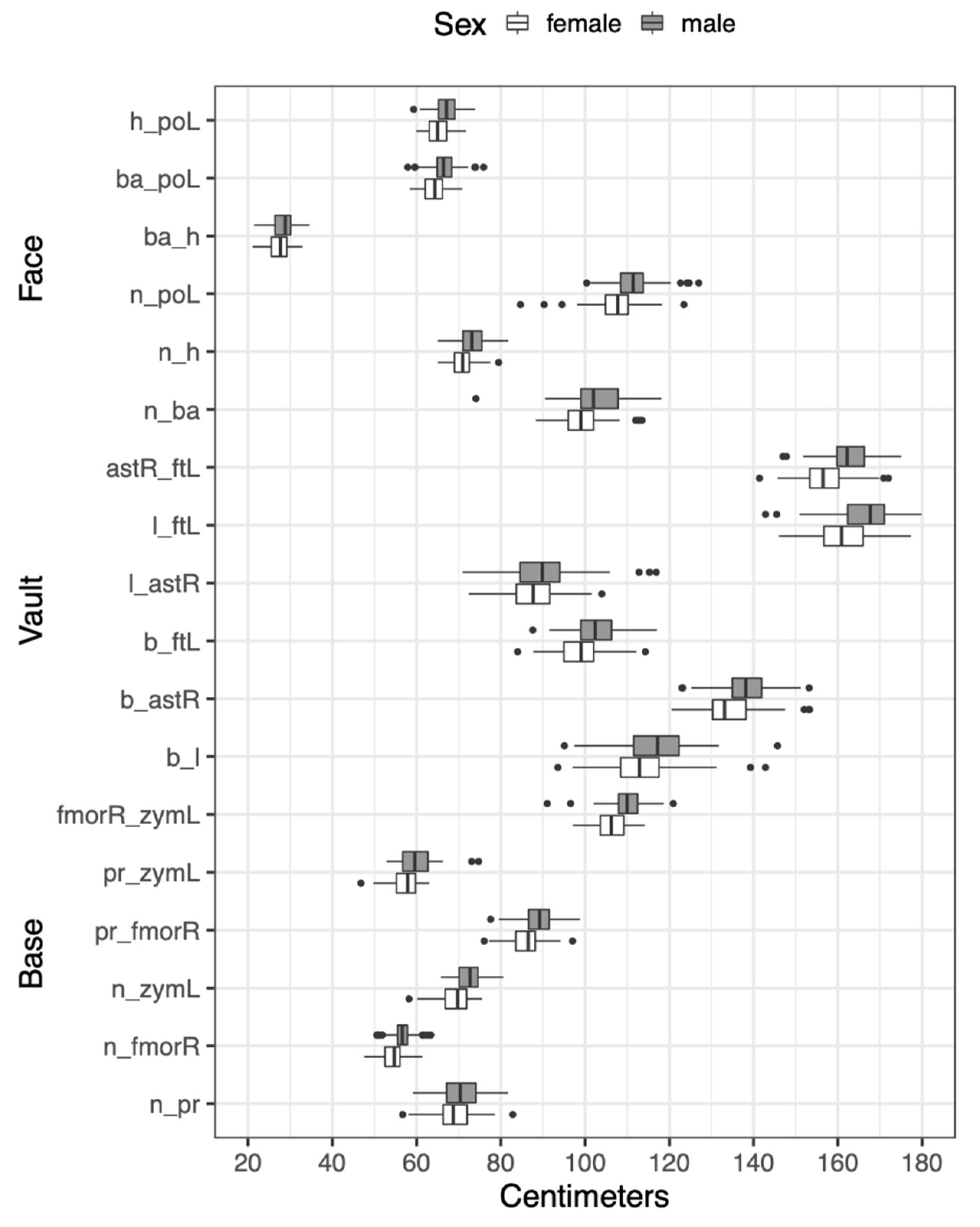
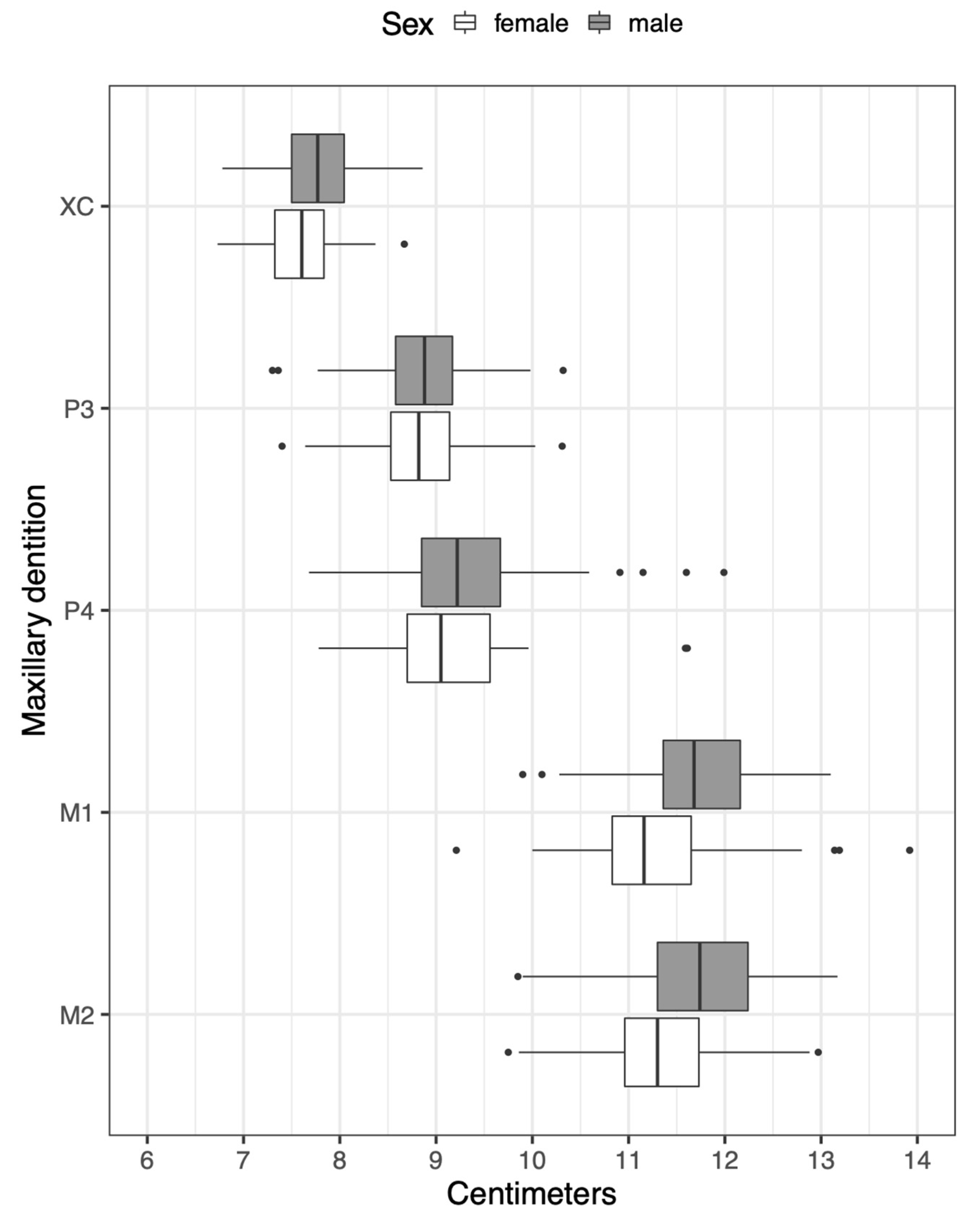
Results indicate that ensemble machine learning has strong potential for sex prediction and yielded AUC-ROC values greater than 0.90 for the cranial metric data and ~0.74 for the dental metric data. Males are larger than females in all dimensions as shown by the Tukey boxplots in Figure 1 and Figure 2 although distributions for the sexes overlap considerably.

AUC-ROC performance for each algorithm along with their standard errors and confidence intervals are shown in

Table 5. Cross-validated AUC-ROC statistics for the six different measurement regions. 0.5 is the equivalent of random guessing; 1 means perfect prediction.

Bony Region	Algorithm	AUC-ROC	Standard Error	Confidence Interval (Lower)	Confidence Interval (Upper)
Face	Mean of Y	0.5000	0.0493	0.4034	0.5966
	Decision tree	0.8069	0.0259	0.7562	0.8577
	Xgboost	0.8998	0.0152	0.8701	0.9295
	Lasso	0.9042	0.0161	0.8727	0.9357
	Logistic regression	0.9088	0.0157	0.8781	0.9395
	Ranger	0.9306	0.0122	0.9066	0.9545
	DiscreteSL	0.9306	0.0122	0.9066	0.9545
	SuperLearner	0.9426	0.0111	0.9208	0.9644
Vault	Mean of Y	0.5000	0.0493	0.4034	0.5966
	Logistic regression	0.8458	0.0200	0.8067	0.8850
	Lasso	0.8486	0.0198	0.8099	0.8873
	Xgboost	0.8690	0.0188	0.8322	0.9058
	Decision tree	0.8998	0.0218	0.8570	0.9425
	DiscreteSL	0.9030	0.0164	0.8709	0.9351
	Ranger	0.9065	0.0158	0.8756	0.9374
	SuperLearner	0.9116	0.0147	0.8827	0.9404
Base	Mean of Y	0.5000	0.0493	0.4034	0.5966
	Logistic regression	0.7667	0.0238	0.7201	0.8132
	Lasso	0.7685	0.0238	0.7219	0.8152
	Decision tree	0.7986	0.0248	0.7500	0.8472
	Xgboost	0.8646	0.0177	0.8298	0.8993
	Ranger	0.9051	0.0146	0.8764	0.9338
	DiscreteSL	0.9051	0.0146	0.8764	0.9338
	SuperLearner	0.9060	0.0146	0.8774	0.9347
Cranial	Mean of Y	0.5000	0.0493	0.4034	0.5966
	Decision tree	0.9125	0.0189	0.8754	0.9496
	Lasso	0.9236	0.0138	0.8966	0.9506
	Logistic regression	0.9282	0.0128	0.9032	0.9533
	Xgboost	0.9306	0.0128	0.9054	0.9557
	Ranger	0.9519	0.0103	0.9317	0.9720
	DiscreteSL	0.9519	0.0103	0.9317	0.9720
	SuperLearner	0.9644	0.0084	0.9480	0.9807
Dental	Mean of Y	0.5000	0.0493	0.4034	0.5966
	Decision tree	0.6537	0.0280	0.5989	0.7086
	Xgboost	0.6551	0.0270	0.6021	0.7081
	Ranger	0.7171	0.0250	0.6680	0.7662
	DiscreteSL	0.7213	0.0256	0.6711	0.7715
	Lasso	0.7412	0.0250	0.6921	0.7903
	Logistic regression	0.7417	0.0252	0.6924	0.7910
	SuperLearner	0.7421	0.0248	0.6935	0.7908
Combined craniodental	Mean of Y	0.5000	0.0493	0.4034	0.5966
	Decision tree	0.9060	0.0196	0.8675	0.9445
	Xgboost	0.9375	0.0116	0.9148	0.9602
	Logistic regression	0.9426	0.0111	0.9209	0.9643
	Lasso	0.9528	0.0104	0.9324	0.9731
	Ranger	0.9549	0.0100	0.9353	0.9745
	DiscreteSL	0.9549	0.0100	0.9353	0.9745
	SuperLearner	0.9722	0.0070	0.9585	0.9860

. The combined craniodental data had the highest AUC-ROC with 0.9722, followed by the combined cranial (0.9644), face (0.9426), vault (0.9116), base (0.9060), and dentition (0.7421). Expectedly, the mean of Y is the worst performing algorithm in all cases (AUC-ROC = 0.500 for each). The SuperLearner algorithm has the highest AUC-ROC for all six bony regions while ranger is a close second for the face, vault, base, cranial, and combined craniodental data. Logistic regression, lasso, and ranger are all close seconds for the dental data.

Additionally, the single best algorithm (or combination of algorithms)—the DiscreteSL—was the ranger random forest algorithm for all 20 cross-validation folds for the face, base, combined cranial data, and combined craniodental data. However, for the vault, ranger was the best performing algorithm 19 times and the decision tree algorithm once. For the dental data, logistic regression was the best performing algorithm 14 times, lasso 4 times, and ranger twice—this algorithmic confusion could be related to the considerably lower AUC-ROC for the dentition compared to any of the cranial data.

The SuperLearner weight distributions show which of the individual algorithms contributed most to the ensemble (

Table 6. Algorithm weight contributions to the SuperLearner ensembles.

Bony Region	Algorithm	Mean (Contribution to Ensemble)	Standard Deviation	Min	Max
Face	Ranger	0.4634	0.1058	0.2389	0.6044
	Logistic regression	0.4193	0.0373	0.3262	0.4779
	Xgboost	0.1159	0.0928	0.0000	0.3199
	Lasso	0.0013	0.0059	0.0000	0.0263
	Decision tree	0.0001	0.0004	0.0000	0.0017
	Mean of Y	0.0000	0.0000	0.0000	0.0000
Vault	Ranger	0.5004	0.1205	0.1910	0.7078
	Decision tree	0.3234	0.0935	0.1591	0.5442
	Logistic regression	0.1412	0.0520	0.0556	0.2234
	Xgboost	0.0350	0.0561	0.0000	0.1483
	Mean of Y	0.0000	0.0000	0.0000	0.0000
	Lasso	0.0000	0.0000	0.0000	0.0000
Base	Ranger	0.8878	0.0701	0.7068	0.9811
	Logistic regression	0.0758	0.0259	0.0189	0.1264
	Xgboost	0.0364	0.0590	0.0000	0.2168
	Mean of Y	0.0000	0.0000	0.0000	0.0000
	Lasso	0.0000	0.0000	0.0000	0.0000
	Decision tree	0.0000	0.0000	0.0000	0.0000
Crania	Ranger	0.4610	0.1162	0.2750	0.6789
	Logistic regression	0.1940	0.0859	0.0299	0.3193
	Lasso	0.1411	0.0753	0.0380	0.2882
	Decision tree	0.1267	0.1028	0.0000	0.3101
	Xgboost	0.0772	0.0826	0.0000	0.2452
	Mean of Y	0.0000	0.0000	0.0000	0.0000
Dental	Logistic regression	0.5591	0.0608	0.4472	0.6747
	Ranger	0.3582	0.0953	0.1797	0.5286
	Decision tree	0.0747	0.0719	0.0000	0.2339
	Xgboost	0.0080	0.0160	0.0000	0.0573
	Mean of Y	0.0000	0.0000	0.0000	0.0000
	Lasso	0.0000	0.0000	0.0000	0.0000
Combined craniodental	Lasso	0.4522	0.0918	0.2598	0.6602
	Ranger	0.1734	0.1048	0.0000	0.3853
	Xgboost	0.1700	0.0739	0.0416	0.2906
	Logistic regression	0.1319	0.0892	0.0000	0.3308
	Decision tree	0.0726	0.0755	0.0000	0.1891
	Mean of Y	0.0000	0.0000	0.0000	0.0000

). For the combined craniodental data, lasso contributed a coefficient of 0.4522, indicating that it contributed this percentage to the SuperLearner ensemble. This was followed by lesser contributes from the ranger algorithm (0.1734), xgboost (0.1700), logistic regression (0.1319), and decision tree (0.0726). For cranial data, ranger contributed a coefficient of 0.4610, followed by lesser contributions from logistic regression (0.1940), lasso (0.1411), decision tree (0.1267), and xgboost (0.0772). Contributions to the face stem mostly from ranger (0.4634) and logistic regression (0.4193), for the vault from ranger (0.5004) and decision tree (0.3234), and for the base from ranger (0.8878). For the dentition, contributions stem mostly from logistic regression (0.5591) and ranger (0.3582).

4. Discussion

AUC-ROC of this SuperLearner ensemble machine learning framework demonstrates strong potential for cranial sex prediction of archaeological human skeletal remains in this particular central Italian context. An important potential contribution of this research is that it reframes the problem of sex estimation as a predictive one and does not rely on assumptions of p-values, traditional hypothesis testing, or causal inference approaches. Instead, the focus was on model performance, standard errors, and confidence intervals. Additionally, the goal here was not to optimize any algorithms for maximum predictive accuracy, but to instead provide a gentle overview of the process and to stimulate the reader into thinking about how this approach could be applied in their own research contexts. This method can also potentially be employed in the field to help resolve disagreements between experts or for indeterminate remains.

Results also support previous research that ensemble machine learning has strong potential for sex prediction in the bioarchaeological record [33]. Although the actual ground truth (in the binary sense; sex and gender are more dynamic than this in reality) male/female sexes of the individuals included in this study were not known, results support previous research that indicates contrasts between male and female morphological and burial patterns in central Italy during the Iron Age [39,40,41]. Among the three different cranial regions, the face had the highest AUC-ROC values, followed by the vault and base. This could provide further support for the utility of the face for population reconstruction despite its greater environmental plasticity compared to the base and vault due to sensory functions of sight, smell, and taste [67].

Of particular interest were the general size differences between males and females. Despite their overlapping measurement distributions—and if the modeling process was strongly influenced by size alone—it would be reasonable to expect that the dentition would have had higher AUC-ROC values similar to those of the cranial data. Whether or not the antimeric substitution of left teeth for right teeth in the absence of a right-side tooth and/or the sheer amount of missingness influenced the much lower dental AUC-ROC is unknown. More cranial-dental comparisons are necessary to evaluate the reliability of the dentition in this framework.

The ensembles themselves can be strengthened by including a greater diversity of algorithms and customizing them with varying hyperparameters (pre-training settings) to find the most accurate and best performing tunings [68]. Other considerations can be more thoroughly incorporated as well, such as different confusion matrix derivations to evaluate performance, such as precision and recall to further highlight class imbalance problems, balanced estimator constructions, false discovery rate, and F1 score. Negative log-likelihood could also be used as the optimizer instead of nonnegative least squares. Other algorithms and methods also might be more appropriate—only a few algorithms with default settings were incorporated in this project but many others can be included in the ensemble (e.g., Bayesian additive regression trees [69]). Features could be screened to identify more interpretable models and custom algorithms can be included to the researcher’s exact specifications (see Kennedy, 2017 [61] for the R walkthrough). Moreover, deep learning—a subdiscipline of machine learning that utilizes multi-layered artificial neural networks for modeling, predicting, inferring, and understanding data—might be even more useful [70]. When dataset sizes and the number of algorithms exceed personal compute potential, the software packages for analyses mentioned in this research have instructions to be run in parallel across multiple cores on a single computer or across multiple machines in cluster or remote settings. Perhaps of great interest to the bioarchaeologist, variable importance information can be extracted from various algorithms to see which cranial and dental dimensions have the highest weights for sex classification.

It is critical to note that due to the antiquity of the samples included in this research, the ground truth sexes of the individuals included were estimated macroscopically using pelvic and skull traits. As a result, future researchers should consider implementing this or similar frameworks using known-sex reference skeletal collections from the Hamann-Todd Osteological Collection (housed at the Cleveland Museum of Natural History), the Robert J. Terry Anatomical Skeletal Collection (Smithsonian Institution, National Museum of Natural History), or the 21st Century Identified Skeletal Collection (University of Coimbra, Portugal). However, my goal was not to concretely establish this ensemble machine learning method in any dogmatic way, but to instead onboard the reader to the basic concepts and their application in bioarchaeology. This study is merely a demonstration of the methods and an advertisement of the potential for generalized low rank imputation and ensemble machine learning processes in bioarchaeological and forensic contexts. Known-sex references samples should be a prerequisite for confirmation of methods presented here, and larger sample sizes might also be important. Cadaver samples and skeletal collections such as those mentioned above would be particularly useful for these procedures. Furthermore, I encourage future researchers to examine the effects that different missing data handling methods (listwise deletion, mean, median, k-nearest neighbor, bootstrap, expectation-maximization, multiple imputation, GLRMs, etc.) have on error estimates in cases of sex prediction in the bioarchaeological record.

Ensemble machine learning techniques should be considered as part of the bioarchaeologist’s toolkit as an additional method for comparison to macroscopic interrogations of the skeleton and dentition that we rely upon for reconstruction of the biological profiles of past humans. These techniques can potentially assist not only in bioarchaeological reconstructions, but also in forensic applications for identification of missing persons and perhaps even to material, faunal, and floral assemblages as well as mortuary studies and settlement organization. Furthermore, GLRMs warrant further exploration and should be considered by bioarchaeologists as a potentially strong data preprocessing tool when faced with missing data and analytical techniques that require full datasets for computation. Social scientists in general would benefit from updating their instrumentation with cross-validated ensemble machine learning techniques when research requires an outcome to be predicted.

References

- Buikstra, J.E.; Ubelaker, D.H. Standards for Data Collection from Human Skeletal Remains; Arkansas Archaeological Survey: Fayetteville, AR, USA, 1994. [Google Scholar]
- Garvin, H.M.; Ruff, C.B. Sexual dimorphism in skeletal browridge and chin morphologies determined using a new quantitative method. Am. J. Phys. Anthr. 2012, 147, 661–670. [Google Scholar] [CrossRef]
- Krishan, K.; Chatterjee, P.M.; Kanchan, T.; Kaur, S.; Baryah, N.; Singh, R.K. A review of sex estimation techniques during examination of skeletal remains in forensic anthropology casework. Forensic Sci. Int. 2016, 261, e1–e165. [Google Scholar] [CrossRef]
- Slemenda, C.W.; Reister, T.K.; Hui, S.L.; Miller, J.Z.; Christian, J.C.; Johnston, C.C. Inluences on skeletal mineralization in children and adolescents: Evidence for varying effects of sexual maturation and physical activity. J. Pediatr. 1994, 125, 201–207. [Google Scholar] [CrossRef]
- Wang, Y. Is Obesity Associated with Early Sexual Maturation? A Comparison of the Association in American Boys Versus Girls. Pediatrics 2002, 110, 903–910. [Google Scholar] [CrossRef] [Green Version]
- Weiss, K.M. On the systematic bias in skeletal sexing. Am. J. Phys. Anthr. 1972, 37, 239–249. [Google Scholar] [CrossRef] [Green Version]
- Sutter, R.C. Nonmetric Subadult Skeletal Sexing Traits: I. A Blind Test of the Accuracy of Eight Previously Proposed Methods Using Prehistoric Known-Sex Mummies from Northern Chile. J. Forensic Sci. 2003, 48, 927–935. [Google Scholar] [CrossRef] [PubMed] [Green Version]
- Konigsberg, L.W.; Algee-Hewitt, B.F.B.; Steadman, D.W. Estimation and evidence in forensic anthropology: Sex and race. Am. J. Phys. Anthr. 2009, 139, 77–90. [Google Scholar] [CrossRef]
- Jackes, M. Representativeness and bias in archaeological skeletal samples. In Social Bioarchaeology; Agarwal, S.C., Glencross, B.A., Eds.; Wiley-Blackwell: West Sussex, UK, 2011; pp. 107–145. [Google Scholar]
- Sierp, I.; Henneberg, M. The Difficulty of Sexing Skeletons from Unknown Populations. J. Anthr. 2015, 2015. [Google Scholar] [CrossRef] [Green Version]
- Irurita Olivares, J.; Alemán Aguilera, I. Validation of the sex estimation method elaborated by Schutkowski in the Granada Osteological Collection of identified infant and young children: Analysis of the controversy between the different ways of analyzing and interpreting the results. Int. J. Leg. Med. 2016, 130, 1623–1632. [Google Scholar] [CrossRef]
- Sjøvold, T. A report on the heritability of some cranial measurements and non-metric traits. In Multivariate Statistical Methods in Physical Anthropology; Van Vark, G.H., Howells, W.W., Eds.; Reidel Publishing Company: Dordrecht, The Netherlands, 1984; pp. 223–246. [Google Scholar]
- Devor, E.J. Transmission of human cranial dimensions. J. Craniofac. Genet. Dev. Biol. 1987, 7, 95–106. [Google Scholar]
- Roseman, C.C. Detecting interregionally diversifying natural selection on modern human cranial form by using matched molecular and morphometric data. Proc. Natl. Acad. Sci. USA 2004, 101, 12824–12829. [Google Scholar] [CrossRef] [Green Version]
- Roseman, C.C.; Weaver, T.D. Multivariate apportionment of global human craniometric diversity. Am. J. Phys. Anthr. 2004, 125, 257–263. [Google Scholar] [CrossRef]
- Carson, E.A. Maximum likelihood estimation of human craniometric heritabilities. Am. J. Phys. Anthr. 2006, 131, 169–180. [Google Scholar] [CrossRef] [PubMed]
- Witherspoon, D.J.; Wooding, S.; Rogers, A.R.; Marchani, E.E.; Watkins, W.S.; Batzer, M.A.; Jorde, L.B. Genetic similarities within and between human populations. Genetics 2007, 176, 351–359. [Google Scholar] [CrossRef] [Green Version]
- Martínez-Abadías, N.; Esparza, M.; Sjøvold, T.; González-José, R.; Santos, M.; Hernández, M. Heritability of human cranial dimensions: Comparing the evolvability of different cranial regions. J. Anat. 2009, 214, 19–35. [Google Scholar] [CrossRef] [PubMed]
- Strauss, A.; Hubbe, M. Craniometric Similarities Within and between Human Populations in Comparison with Neutral Genetic Markers. Hum. Biol. 2010, 82, 315–330. [Google Scholar] [CrossRef] [PubMed]
- Herrera, B.; Hanihara, T.; Godde, K. Comparability of multiple data types from the Bering Strait region: Cranial and dental metrics and nonmetrics, mtDNA, and Y-Chromosome DNA. Am. J. Phys. Anthr. 2014, 54, 334–348. [Google Scholar] [CrossRef] [PubMed]
- Buikstra, J.E.; Frankenberg, S.R.; Konigsberg, L.W. Skeletal biological distance studies in American Physical Anthropology: Recent trends. Am. J. Phys. Anthr. 1990, 82, 1–7. [Google Scholar] [CrossRef]
- Cunningham, S.J. Machine learning applications in anthropology: Automated discovery over kinship structures. Comput. Humanit. 1996, 30, 401–406. [Google Scholar] [CrossRef]
- Bell, S.; Jantz, R. Neural network classification of skeletal remains. In Archaeological Inormatics: Pushing the Envelope; Burenhult, G., Ed.; Archaeopress: Oxford, UK, 2001; pp. 205–212. [Google Scholar]
- Hefner, J.T.; Ousley, S.D. Statistical Classification Methods for Estimating Ancestry Using Morphoscopic Traits. J. Forensic Sci. 2014, 59, 883–890. [Google Scholar] [CrossRef]
- Czibula, G.; Ionescu, V.S.; Miholca, D.L.; Mircea, I.G. Machine learning-based approaches for predicting stature from archaeological skeletal remains using long bone lengths. J. Archaeol. Sci. 2016, 69, 85–99. [Google Scholar] [CrossRef]
- Ionescu, V.S.; Teletin, M.; Voiculescu, E.M. Machine learning techniques for age at death estimation from long bone lengths. In Proceedings of the 2016 IEEE 11th International Symposium on Applied Computational Intelligence and Inormatics (SACI), Timisoara, Romania, 12–14 May 2016; pp. 457–462. [Google Scholar]
- Ionescu, V.S.; Czibula, G.; Teletin, M. Supervised Learning Techniques for Body Mass Estimation in Bioarchaeology. In Soft Computing Applications—Advances in Intelligent Systems and Computing 634; Balas, V., Jain, L., Balas, M., Eds.; Springer: Berlin/Heidelberg, Germany, 2018. [Google Scholar]
- Miholca, D.L.; Czibula, G.; Mircea, I.G.; Czibula, I.G. Machine learning based approaches for sex identification in bioarchaeology. In Proceedings of the 18th International Symposium on Symbolic and Numeric Algorithms for Scientific Computing (SYNASC), Timisoara, Romania, 24–27 September 2016; pp. 311–314. [Google Scholar]
- Pink, C.M. Forensic Ancestry Assessment Using Cranial Nonmetric Traits Traditionally Applied to Biological Distance Studies. In Biological Distance Analysis–Forensic and Bioarchaeological Perspectives; Pilloud, M.A., Hefner, J.T., Eds.; Academic Press: San Diego, CA, USA, 2016; pp. 213–230. [Google Scholar]
- Porto, F.P.; Lima, L.N.C.; Flores, M.R.P.; Valsecchi, A.; Ibanez, O.; Palhares, C.E.M.; de Barros Vidal, F. Automatic cephalometric landmarks detection on frontal faces: An approach based on supervised learning techniques. Digit. Investig. 2019, 30, 108–116. [Google Scholar] [CrossRef] [Green Version]
- Ortiz, A.G.; Costa, C.; Silva, R.H.A.; Biazevic, M.G.H.; Michel-Crosato, E. Sex estimation: Anatomical references on panoramic radiographs using machine learning. Forensic Imaging 2020, 20, 200356. [Google Scholar] [CrossRef]
- Kenyhercz, M.W.; Passalacqua, N.V. Missing Data Imputation Methods and Their Performance with Biodistance Analyses. In Biological Distance Analysis–Forensic and Bioarchaeological Perspectives; Pilloud, M.A., Hefner, J.T., Eds.; Academic Press: San Diego, CA, USA, 2016; pp. 181–194. [Google Scholar]
- Muzzall, E.; Kennedy, C.J.; Culich, A. Ensemble Machine Learning for Sex Prediction of a Worldwide Craniometric Dataset, Poster Presented at the Berkeley Institute for Data Science Data Science Faire. Available online: https://github.com/EastBayEv/Ensemble-machine-learning-for-sex-prediction-of-a-worldwide-craniometric-dataset (accessed on 7 July 2020).
- Scozzari, R.; Cruciani, F.; Pangrazio, A.; Santolamazza, P.; Vona, G.; Moral, P.; Latini, V.; Varesi, L.; Memmi, M.M.; Romano, V.; et al. Human Y-chromosome variation in the Western Mediterranean area: Implications for the peopling of the region. Hum. Immunol. 2001, 62, 871–884. [Google Scholar] [CrossRef] [Green Version]
- Coppa, A.; Cucina, A.; Lucci, M.; Mancinelli, D.; Vargiu, R. Origins and spread of agriculture in Italy: A nonmetric dental analysis. Am. J. Phys. Anthr. 2007, 133, 918–930. [Google Scholar] [CrossRef]
- Muttoni, G.; Scardia, G.; Kent, D.V.; Swisher, C.C.; Manzi, G. Pleistocene magnetochronology of early hominin sites at Ceprano and Fontana Ranuccio, Italy. Earth Planet Sci. Lett. 2009, 286, 255–268. [Google Scholar] [CrossRef] [Green Version]
- Fu, Q.; Rudan, P.; Pääbo, S.; Krause, J. Complete Mitochondrial Genomes Reveal Neolithic Expansion into Europe. PLoS ONE 2012, 7, e32473. [Google Scholar] [CrossRef] [Green Version]
- Ghirotto, S.; Tassi, F.; Fumagalli, E.; Colonna, V.; Sandionigi, A.; Lari, M.; Vai, S.; Petiti, E.; Corti, G.; Rizzi, E.; et al. Origins and Evolution of the Etruscans’ mtDNA. PLoS ONE 2013, 8, e55519. [Google Scholar] [CrossRef] [PubMed] [Green Version]
- Muzzall, E.; Coppa, A. Temporal and Spatial Biological Kinship Variation at Campovalano and Alfedena in Iron Age Central Italy. In Bioarcheology of Frontiers and Borderlands; Tica, C., Martin, D.L., Eds.; University Press of Florida: Gainesville, FL, USA, 2019; pp. 107–132. [Google Scholar]
- Coppa, A.; Macchiarelli, R. The maxillary dentition of the Iron-Age population of Alfedena (Middle-Adriatic Area, Italy). J. Hum. Evol. 1982, 11, 219–235. [Google Scholar] [CrossRef]
- Bondioli, L.; Corruccini, R.S.; Macchiarelli, R. Familial segregation in the Iron Age community of Alfedena, Abruzzo, Italy, based on osteodental trait analysis. Am. J. Phys. Anthr. 1986, 71, 393–400. [Google Scholar] [CrossRef]
- Hillson, S.; FitzGerald, C.; Flinn, H. Alternative dental measurements: Proposals and relationships with other measurements. Am. J. Phys. Anthr. 2006, 126, 413–426. [Google Scholar] [CrossRef]
- Udell, M.; Horn, C.; Zadeh, R.; Boyd, S. Generalized Low Rank Models. Found. Trends Mach. Learn. 2016, 9, 1–118. [Google Scholar] [CrossRef]
- James, G.; Witten, D.; Hastie, T.; Tibshirani, R. An Introduction to Statistical Learning: With Applications in R.; Springer: New York, NY, USA, 2013. [Google Scholar]
- Breiman, L. Statistical Modeling: The Two Cultures. Stat. Sci. 2001, 16, 199–231. [Google Scholar] [CrossRef]
- Welling, M. Are ML and Statistics Complimentary? Roundtable Discussion at the 6th IMS-ISBA Meeting on Data Science in the Next 50 Years; University of Amsterdam: Amsterdam, The Netherlands, 2015. [Google Scholar]
- Turing, A.M. Computing Machinery and Intelligence. Mind 1950, 59, 433–460. [Google Scholar] [CrossRef]
- Rosenblatt, F. The perceptron: A probabilistic model for information storage and organization in the brain. Psychol. Rev. 1958, 65, 386–408. [Google Scholar] [CrossRef] [Green Version]
- Samuel, A.L. Some Studies in Machine Learning Using the Game of Checkers. IBM J. Res. Dev. 1959, 3, 207–226. [Google Scholar] [CrossRef]
- Dietterich, T.G. Ensemble methods in machine learning. In Lecture Notes in Computer Science 1857; Goos, G., Hartmanis, J., van Leeuwen, J., Eds.; Springer: Berlin/Heidelberg, Germany, 2000; pp. 1–15. [Google Scholar]
- Van der Laan, M.J.; Polley, E.C.; Hubbard, A.E. Super Learner. Stat. Appl. Genet. Mol. Biol. 2007, 6, 1–21. [Google Scholar] [CrossRef] [PubMed]
- Polley, E.C.; van der Laan, M.J. Super Learner in Prediction, UC Berkeley Division of Biostatistics Working Paper Series Paper 266. Available online: https://biostats.bepress.com/ucbbiostat/paper266 (accessed on 8 September 2020).
- Efron, B.; Gong, G. A Leisurely Look at the Bootstrap, the Jackknife, and Cross-Validation. Am. Stat. 1982, 37, 36–48. [Google Scholar] [CrossRef]
- Dobson, A.J. An Introduction to Generalized Linear Models; Chapman and Hall: London, UK, 1990. [Google Scholar]
- Friedman, J.; Hastie, T.; Tibshirani, R. Regularization Paths for Generalized Linear Models via Coordinate Descent. J. Stat. Softw. 2010, 33, 1–22. [Google Scholar] [CrossRef] [Green Version]
- Breiman, L.; Friedman, J.; Olshen, R.; Stone, C. Classification and Regression Trees; Wadsworth: Belmont, CA, USA, 1984. [Google Scholar]
- Breiman, L. Random Forests. Mach. Learn. 2001, 45, 5–32. [Google Scholar] [CrossRef] [Green Version]
- Wright, N.; Ziegler, A. ranger: A fast implementation of random forests for high dimensional data in C++ and R. J. Stat. Softw. 2017, 77, 1–17. [Google Scholar] [CrossRef] [Green Version]
- Freund, Y.; Schapire, R.E. A Short Introduction to Boosting. J. Jpn. Soc. Art. Int. 1999, 14, 1–14. [Google Scholar]
- Chen, T.; He, T.; Benesty, M.; Khotilovich, V.; Tang, Y.; Cho, H.; Chen, K.; Mitchell, R.; Cano, I.; Zhou, T.; et al. Xgboost: Extreme Gradient Boosting, R Package, 2019, Version 0.90.0.2. Available online: https://CRAN.R-project.org/package=xgboost (accessed on 26 September 2020).
- Kennedy, C. Guide to SuperLearner. 2017. Available online: https://cran.r-project.org/web/packages/SuperLearner/vignettes/Guide-to-SuperLearner.html (accessed on 26 September 2020).
- Lantz, B. Machine Learning with R.; Packt Publishing: Birmingham, UK, 2015. [Google Scholar]
- Hanley, J.A.; McNeil, B.J. The meaning and use of the area under a receiver operating characteristic (ROC) curve. Radiology 1982, 143, 29–36. [Google Scholar] [CrossRef] [Green Version]
- Wickham, H. Ggplot2: Elegant Graphics for Data Analysis; Springer: New York, NY, USA, 2016. [Google Scholar]
- Polley, E.; LeDell, E.; Kennedy, C.; van der Laan, M. SuperLearner: Super Learner Prediction, R Package Version 2.0-26. 2019. Available online: https://CRAN.R-project.org/package=SuperLearner (accessed on 21 November 2020).
- Kennedy, C. Ck37r: Chris Kennedy’s R Toolkit, R Package Version 1.0.3. 2020. Available online: https://github.com/ck37/ck37r (accessed on 10 March 2020).
- Taubadel, N.V.C. Revisiting the homoiology hypothesis: The impact of phenotypic plasticity on the reconstruction of human population history from craniometric data. J. Hum. Evol. 2009, 57, 179–190. [Google Scholar] [CrossRef]
- Bergstra, J.; Bengio, Y. Random Search for Hyper-Parameter Optimization. J. Mach. Learn. Res. 2012, 13, 281–305. [Google Scholar]
- Chipman, H.A.; George, E.I.; McCulloch, R.E. BART: Bayesian additive regression trees. Ann. Appl. Stat. 2010, 1, 266–298. [Google Scholar] [CrossRef]
- Chollet, F.; Allaire, J.J. Deep Learning with R.; Manning: New York, NY, USA, 2017. [Google Scholar]
Figure 1.
Distributions of raw cranial data for males and females. Cranial landmark abbreviations are defined in Table 2.
Figure 2.
Distributions of raw dental data for males and females. Dental distance abbreviations are defined in Section 2.1.