Article

On the Sliding Mode Control Applied to a DC-DC Buck Converter

by
Sandra Huerta-Moro
1,†,
Oscar Martínez-Fuentes
1,†,
Victor Rodolfo Gonzalez-Diaz
2,† and
Esteban Tlelo-Cuautle
1,*,†
1
Electronics Department, Instituto Nacional de Astrofísica, Optica y Electrónica (INAOE), Luis Enrique Erro No. 1, Tonantzintla, Puebla 72840, Mexico
2
Faculty of Electronics Sciences, Benémerita Universidad Autónoma de Puebla (BUAP), Puebla 72570, Mexico
*
Author to whom correspondence should be addressed.
These authors contributed equally to this work.
Technologies 2023, 11(2), 33; https://doi.org/10.3390/technologies11020033
Submission received: 24 December 2022 / Revised: 17 February 2023 / Accepted: 22 February 2023 / Published: 23 February 2023

Abstract

:
This work shows the voltage regulation of a DC–DC buck converter by applying sliding mode control using three different cases of sliding surfaces. The DC–DC buck converter is modeled by ordinary differential equations (ODEs) that are solved by applying numerical methods. The ODEs describe two state variables that are associated to the capacitor voltage and the inductor current. The state variable associated to voltage is regulated by applying two well-known sliding surfaces and a third one that is introduced herein to improve the response of the sliding mode control. The stability of the proposed sliding surface is verified by using a Lyapunov theorem to guarantee closed-loop stability. Finally, simulation results show the improvement of voltage regulation when applying the proposed sliding surface compared to already reported approaches.

1. Introduction

The majority of works related to converters in the direct current (DC) domain agree that they are the most significant part of any hybrid renewable energy system. DC–DC converters are used to stabilize a desired value considered as voltage output, which is subject to some intermittent conditions and nonidealities of the circuit elements and of the switches. During the conversion process, some desirable characteristics qualify the performance of such systems—one of them is the power quality of renewable energy systems, which heavily relies on the stable operation of the power converter and its control technique. On these issues, the authors in [1], published a good review paper that helps to understand the classification of non-isolated DC–DC converters and their control techniques for renewable energy applications. In that work, it is noticed that most of the conventional converters and control techniques have several disadvantages for real applications, meaning that one must evaluate the efficacy when they are applied to a particular system. On the one hand, some research has been done to improve or to introduce new DC–DC converter topologies to accomplish target specifications [2]; on the other hand, another problem is the implementation of the control to guarantee a desired voltage output. With this in mind, electronics-based DC–DC converters are considered to be more efficient than the conventional power conversion techniques.
One of the main problems of DC–DC converters is the design of the control technique to improve their performances and correct operation. On this issue, the authors in [1] provide a brief classification and discussion of several control techniques, mentioning that the design of the control is highly significant since it plays a vital role in evaluating the performance of DC–DC converters in renewable energy applications. The authors provide several recommendations as a comparative analysis among different control techniques and their performance on various DC–DC converters, considered as non-isolated ones. In this manner, one can find generic topologies of conventional DC–DC converters that include buck, buck-boost, single ended primary inductor converter (SEPIC), cuk, z-source, zeta converter and the interleaved DC–DC converter. These topologies are classified according to some relevant characteristics that are related to the high-efficiency high step-up, high gain input-parallel output-series, high gain transformer-less double-duty-triple-mode and high gain three-state switching hybrid boost converter. From the issues mentioned above, it can be inferred that DC–DC conversion is one of the most studied and applied methods in the area of power electronics, in which the DC–DC buck converter is one of the well-known circuits. The objective of the step down DC–DC buck converter is to regulate the output voltage to a reference value, even with the non-ideal characteristics of the circuit elements and changes on the load conditions. Basically, the buck converter topology is one of the simplest but most useful power converters that can convert a DC input to a DC output at a lower voltage. The versatility of this converter makes it suitable for low and high-power applications. Among the main applications of the DC–DC buck converters, one can see their use in micro-grids [3,4,5,6], renewable energy systems [1,7,8], photovoltaic systems and battery charging [9,10], LED driver and energy management [11,12], speed control of DC and AC motor drivers [2,13] and so on.
One of the main objectives of most closed-loop feedback-controlled DC–DC converters is to ensure that the converter operates with fast dynamic response, small steady-state output error and low overshoot while maintaining high efficiency and low noise emission in terms of the rejection of input voltage changes uncertainties and load variations [14]. In this regard, the frequently used control methods applied to DC–DC converters can be associated to proportional–integral–derivative (PID) [2,4,5] and feedback linearization [3,4,15]. However, linear control methods require the plant to be linearized and thus are quite sensitive to external variations and uncertainties. These problems can be mitigated by applying non-linear control methods, which improve transient response. Some of the currently applied non-linear control methods are, for example, optimal control [3], model predictive control (MPC) [1], neuronal network, extended state observer based control [8], fuzzy logic control (FLC) [7,9], passivity-based control [12], sliding mode control (SMC) [16], twisting based SMC [6,11] and sliding mode observer [17]. In this paper, it is shown that the DC–DC buck converter is highly effective for DC voltage regulation, and the desired voltage output is ensured by implementing an SMC considering three different cases of the control law. Henceforth, this work shows that SMC theory is a powerful tool to design effective control laws. The next sections show that the dynamics of the sliding mode depend on the switching of the surface and not on the control. In this manner, the DC–DC buck converter is taken as a case study, and the associated sliding mode surface equation is selected to design the desired dynamics of the movement, according to some performance criteria. Therefore, this work highlights that the main advantages of the SMC include robustness, reduced-order compensated dynamics, finite-time convergence and low sensitivity to system parameter variations. To show these advantages, a sliding mode controller to regulate voltage in the buck converter is proposed herein. Basically, a new sliding surface is introduced, considering errors in voltage and current outputs for which simulation results are provided and compared to two cases that have been already published.
The manuscript is organized as follows: Section 2 shows the DC–DC buck converter topology, which is used to apply the SMC method considering three cases. Two cases are already known, and a third one is introduced herein, the stability analysis of which is presented in Section 3. Section 4 shows simulation results of the stability analysis by the Lyapunov method, the finite-time convergence and the regulated output voltage without overshoot. Finally, the conclusions are summarized in Section 5.

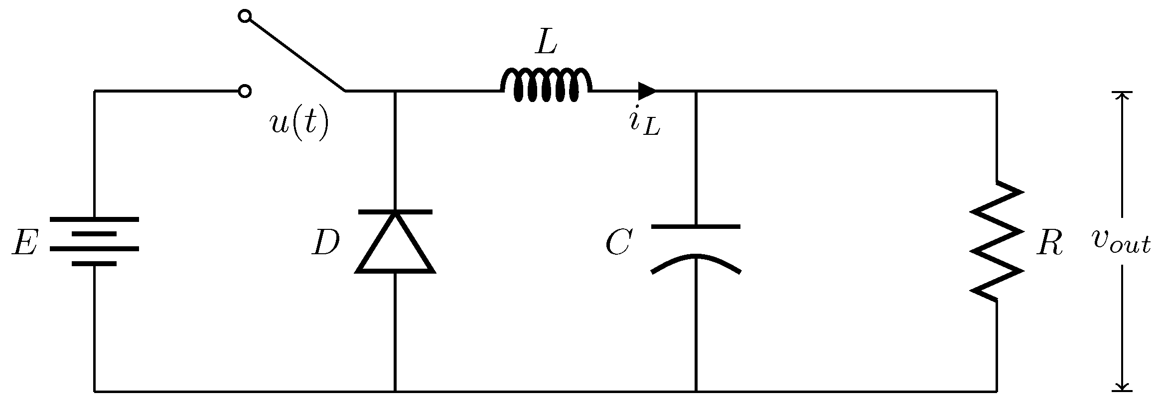
2. DC–DC Buck Converter and Its Smc

The case study herein is the DC–DC buck converter topology shown in Figure 1. It consists of an independent voltage source V, considered as the input; a switch that can be replaced by an active device controlled by a digital signal to be closed or open; a diode and three passive elements, namely an inductor (L), a capacitor (C) and a resistor (R), which models the load to which the desired or output voltage is provided.
The dynamic model of the DC–DC buck converter shown in Figure 1 is described by the two ordinary differential equations (ODEs) given in (1). The control signal u ( t ) takes a logic value so that 1 means closed and 0 means open. The switch can be implemented with an active device such as a transistor, and it is governed by a control block that in this paper is devoted to an SMC. Taking the circuit state variables as x 1 = i L to denote the current through the inductor and x 2 = V C = v o u t to denote the voltage across the capacitor, which also becomes the desired output voltage, one can define the state space as given in (2).
i ˙ L = V C L + u E L V ˙ C = i L C V C R C
x ˙ 1 = 1 L x 2 + u E L x ˙ 2 = 1 C x 1 1 R C x 2
In this work, the state variables are sensed to be controlled by a SMC block, for which three different sliding surfaces are applied herein, and they are described in the following subsections. Two cases are already reported in [4,14], and the third is a proposed new one.

2.1. Case A Given in [4]

Lets us consider the ODEs describing the DC–DC buck converter given in (1). One can perform a variable change [14], where the new variable can be associated to the output voltage or V C minus the desired output regulated voltage expressed by V d . In this case, the new variable is given in (3), which describes the voltage error that is controlled by an SMC block. The derivative of y 1 leads us to (4), where it can be appreciated that the constant value of V d has been eliminated, and afterwards, the derivative of y 2 produces (5).
y 1 = V C V d
y ˙ 1 = V ˙ c = i L C V C R C = y 2
y ˙ 2 = 1 C V C L + u E L 1 R C i L C V C R C = 1 L C u E y 1 V d y 2 R C
According to [14], the change of variables is now described by (6), and it can be used to define a sliding surface s, as denoted in (7). In the sliding surface, α is a positive constant and 0 < β < 1 . Now, the derivative of s is given in (8).
y ˙ 1 = y 2 y ˙ 2 = 1 L C u E y 1 V d y 2 R C
s = α y 1 β + y 2
s ˙ = α β y 1 β 1 y ˙ 1 + y ˙ 2
The control function u can be divided into two parts: the first one is an equivalent and continuous function that generates an invariant surface u e q , and the second one includes the switched system u s , so that it can be expressed by (9), and each term is described as follows:
u = u e q + u s
  • u e q : The equivalent control function is obtained from (8), and according to SMC theory [18], it can be equated to zero to get (10). Replacing the state variables, one gets (11), and afterwards the expression to u is given in (12).
    s ˙ = α β y 1 β 1 y ˙ 1 + y ˙ 2 = 0
    α β y 1 β 1 y 2 + 1 L C u E y 1 V d y 2 R C = 0
    u = y 2 R C α β y 1 β 1 y 2 L C E + V d + y 1 E = u e q
  • u s : In this work, u s is given in (13), where K is a control gain and it can take values to guarantee stability conditions. In the following sections, some values of this gain are given.
    u s = K sign ( s )
The combination of u e q and u s generates the control law described by (14). This is the signal error that is used to control the switch, which can be governed by a comparator with a threshold equal to zero to provide a logic 1 or a logic 0 to close or to open the switch, respectively.
u = y 2 R C α β y 1 β 1 y 2 L C E + V d + y 1 E K sign ( s )

2.2. Case B Given in [14]

In this case, the sliding surface considers the error voltage defined by a new state variable labeled as z 1 and given in (15). The derivative of this variable z 1 is given in (16), where one can appreciate that the derivative of the desired voltage V ˙ d is included in the equation simply to derive an equation similar to that in the work given in [14].
z 1 = V C V d
z ˙ 1 = V ˙ C V ˙ d
One can take z 2 as given in (17), and its derivative is described in (18), where again the second derivative of the desired voltage is included simply to have an equation that may consider this voltage as variable.
z 2 = i L C V C R C V ˙ d
z ˙ 2 = i ˙ L C V ˙ c R C V ¨ d
Replacing the dynamics of (1) into (18), one gets (19), and from (15), one gets (20).
z ˙ 2 = V C L + E L u 1 C i L C V C R C 1 R C V ¨ d
V C = z 1 + V d
From (17), z 2 + V ˙ d is given in (21), and using (20) and (21) in (18), one gets (22).
z 2 + V ˙ d = i L C V C R C
z ˙ 2 = ( z 1 + V d ) L + E L u 1 C z 2 + V ˙ d 1 R C V ¨ d
Defining a = 1 C L and b = 1 R C , the state space is given in (23). One can see that the first and second-order derivatives of V d appearing in (22) have been eliminated since in this work V d is considered as a constant value. However, for cases where the desired value varies, it should be considered as already shown in [14].
z ˙ 1 = z 2 z ˙ 2 = a z 1 a V d + a u E b z 2
Defining the sliding surface as a linear combination of the state variables [4], one gets (24), where c is a positive gain constant, meaning that the derivate of s, considered as the surface, is given by (25).
s = z 1 + c z 2
s ˙ = z ˙ 1 + c z ˙ 2
The control function u is divided again into two parts, as done in the previous case, as given in (9). The two terms u e q and u s are described as follows:
  • u e q : To get the equivalent control function, and according to SMC theory [18], (25) is updated to (26), and the replacement of z ˙ 1 and z ˙ 2 leads us to (27), so that u is given in (28).
    s ˙ = z ˙ 1 + c z ˙ 2 = 0
    s ˙ = z 2 + c ( a z 1 a V d + a E u b z 2 ) = 0
    u = 1 a E ( 1 c z 2 a z 1 a V d b z 2 ) = u e q
  • u s : Considering that u s is given in (29), and by replacing (28) and (29) into (9), the control law function is given in (30). Again, as for case A, u is the signal error that governs a comparator with a threshold equal to zero, thus providing a logic 1 or logic 0 to close or to open the switch of the DC–DC buck converter shown in Figure 1, respectively.
    u s = K sign ( s )
u = 1 a E 1 c z 2 a z 1 a V d b z 2 b V ˙ d V ¨ d K sign ( s )

2.3. Case C: Proposed Sliding Surface

As the target of the control is to provide a constant voltage output V o u t , equal to the desired one V d , then the DC–DC buck converter must be in steady state, which can be accomplished through the condition x 2 = V d , so that x ˙ 2 = 0 .
Assuming that x 1 in x ˙ 2 is an input control, it is possible to denote the desired current as x 1 * . However, x 1 can be expressed in terms of x 2 in order to control the voltage output. This means that the desired current can be expressed by (31). Now, the surface s can be described by ensuring that x 1 tracks the desired current, and therefore, it must accomplish (32). In this manner, when s = 0 , it means that the current is in a stable point, and the voltage loop is in equilibrium when (33) is accomplished.
x 1 * = V d R
s 1 = x 1 x 1 * 0
s 2 = x 2 V d 0
With the goal of forcing the sliding surface during the condition s = 0 , the control u is restricted to take values as 1 or 0. Therefore, in (2), the control is defined according to [18] to get (34), where s is the scalar switched function defined in the sliding mode theory.
u = 1 2 ( 1 sign ( s ) )
The control includes both sliding surfaces (32) and (33), meaning that (34) can be applied to the current and voltage surfaces to get (35). In order to achieve the exponential convergence of the state variables, one has to drive s given in (35) to zero in finite time by means of the control law that is proposed by (36).
s = α s 1 + β s 2
u = 1 2 ( 1 sign ( α s 1 + β s 2 ) )

3. Stability Analysis

The stability analysis for the sliding surfaces described in Section 2.1 and Section 2.2 can be found in Ref. [14] and Ref. [4], respectively. This section describes the stability and convergence analysis for the proposed surface given in Section 2.3.
Theorem 1.
Considering the system given in (1) and the sliding surface given in (35), if the control law is proposed as (36), then the state variables of the system converge to s in a finite time.
Proof of Theorem 1.
In order to prove Theorem 1, the Lyapunov theorem given in [19,20] is applied.
The Lyapunov candidate function is defined in (37), and its time derivative is given in (38).
V = 1 2 s 2
V ˙ = s · s ˙ = s ( α x 1 ˙ + β x 2 ˙ ) = s α L + β R C x 2 + β C x 1 + α E 2 L + s α E L u = s α L + β R C x 2 + β C x 1 + α E 2 L α E 2 L s
For the sliding mode to exist in s = 0 , it is necessary to satisfy the sliding condition s · s ˙ < 0 given in (39), which defines an attraction domain of a sliding manifold. Equation (36) is used to understand the absolute value of s.
s · s ˙ = s α L + β R C x 2 + β C x 1 α E 2 L s < 0
From the inequality in (39), if the sliding mode exists, then the relations given in (40) hold.
s ˙ s > 0 = α L + β R C x 2 + β C x 1 < 0 s ˙ s < 0 = α L + β R C x 2 β C x 1 < α E L
To design the gains α and β , and in order to ensure that (40) is always fulfilled, one can propose the coefficient relationships expressed by (41). In this manner, as the circuit parameters R , L , C , E are known values, as the ones given in Table 1, then replacing the circuit values into (40) results in (42). In this case, as x 2 > x 1 , because the voltage across the capacitor is higher than the current through the inductor, the relationship between α and β can be expressed by the constraint given in (43).
α L > β R C α L + β R C > β C
50 α + 133.3 β x 2 + ( 10000 β ) x 1 < 0 50 α + 133.3 β x 2 ( 10000 β ) x 1 < 250 α
β < 0.0051 α
From (43), it is clear that α holds a relation with β , which implies that α needs to be large enough. Assuming α = 500 , then β < 0.0051 ( 500 ) = 2.55 . If β = 1 , and this value is replaced in (42), both inequalities are fulfilled. In this manner, one can ensure that the stability condition is guaranteed.
Another important issue is the finite-time convergence, which in this case is accomplished beginning by modifying V ˙ < 0 [21], which becomes (44), meaning that over the time interval 0 τ t , one gets (45).
V ˙ γ V 1 2
d V d τ γ V 1 2 2 V ( t ) 1 2 V ( x 0 ) 1 2 γ t V ( t ) 1 2 1 2 γ t + V ( x 0 ) 1 2
Then, V ( t ) reaches zero in a finite time t r , which is given in (46). Therefore, the control will drive the variable s to zero in finite time and will keep it at zero thereafter [21].
t r 2 V ( x 0 ) 1 2 γ
According to (38), the equation can be divided as given in (47) to find boundaries. For the first term, the considerations given in (48) are made, and replacing (48) in (38), one gets (49).
V ˙ = s · s ˙ = s α L + β R C x 2 + β C x 1 + s α E L u
0 < x 2 < E x 1 = x 2 / R
s α L + β R C x 2 + β C x 1 = s α R L + β C x 1 + β C x 1 = | s | α R L x 1
For the second term in (47), substituting u, one gets (50), which leads to the cases given in (51). Consequently, one gets (52), and by adding (49) and (52), one gets (53).
s α E L u = s α E 2 L α E 2 L sign ( s )
s α E 2 L α E 2 L sign ( s ) = 0 if sign ( s ) = 1 s α E 2 L α E 2 L sign ( s ) = | s | α E L if sign ( s ) = 1
s α E L u | s | α E L
V ˙ = s α L + β R C x 2 + β C x 1 + s α E L u V ˙ | s | α R L x 1 + | s | α E L = | s | α R L x 1 + α E L
Taking (37) and (44), one can describe (54), and considering the condition given in (48), the inequality given in (55) is generated, meaning that one gets (56). As a result, the system achieves finite time convergence according to (57), meaning that the state variables converge to s = 0 asymptotically.
2 V = s 2 2 V = | s | V ˙ γ 2 | s | = | s | α R L x 1 + α E L
E L > x 1 R L α R L x 1 + α E L > 0
γ 2 = α R L x 1 α E L γ = 2 α R L x 1 α E L
t r 2 V ( x 0 ) 1 2 2 α R L x 1 α E L

4. Simulation and Discussion of Results

In order to show the performance of the three surfaces described in Section 2, the DC–DC buck converter system has been tested by MATLAB T M simulations. The nominal parameter values of the components and gains are summarized in Table 1 and Table 2—they are values already used in the work given in [4] for case A and in [14] for case B. Besides, one can propose other values or sweep those around the ones already tested, as shown in [2], where the authors vary L and C. In Table 2, one can see two sets of values given for the surfaces of cases A and B, and just one set of values for the proposed surface (case C).

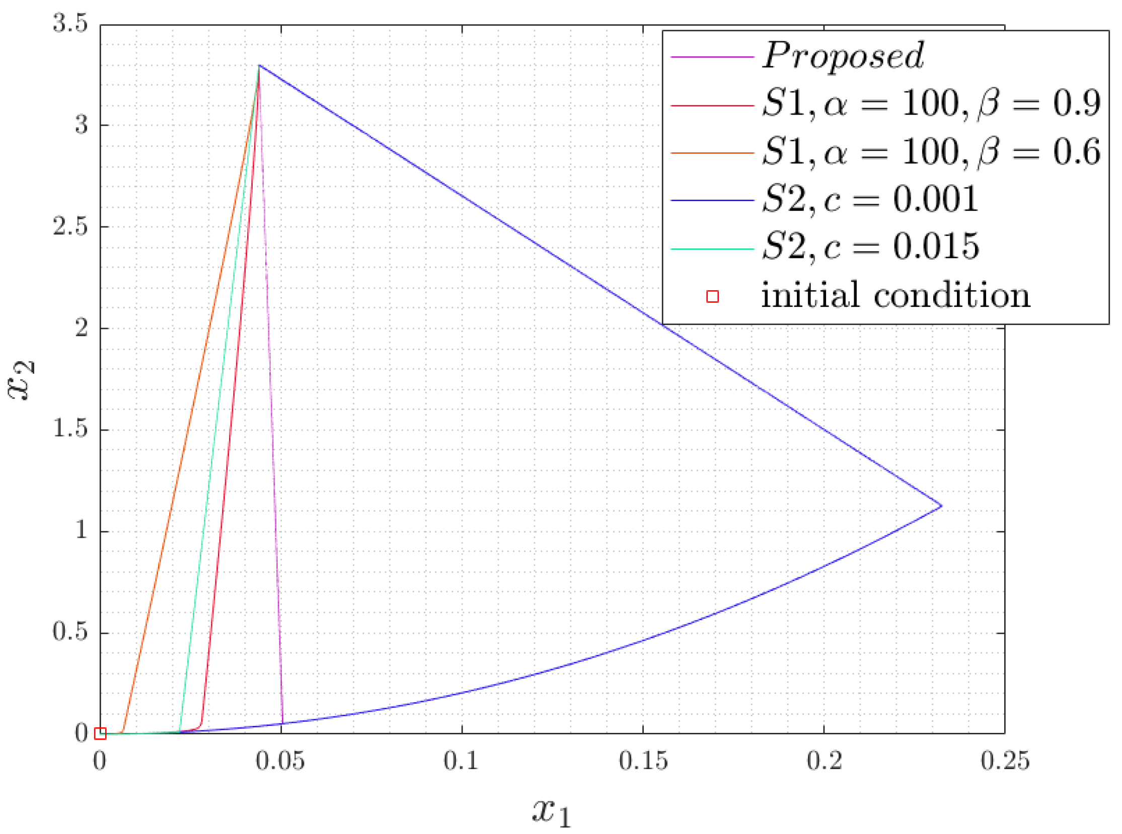
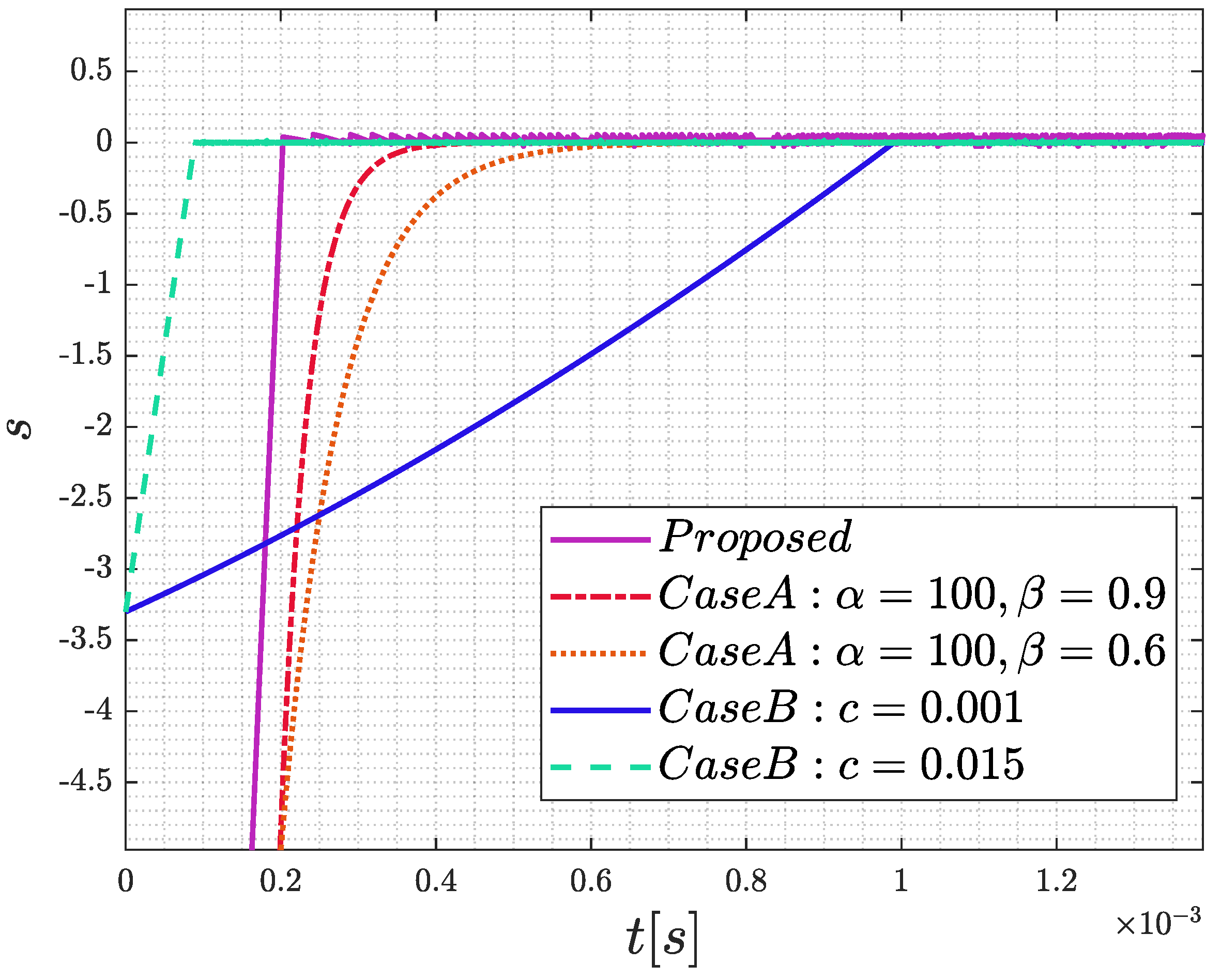
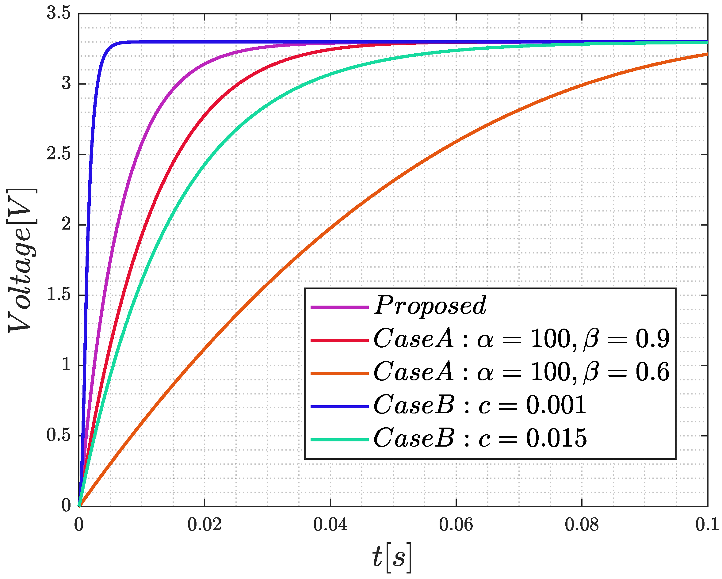
4.1. Numerical Simulation

The numerical simulation of the DC–DC buck converter modeled by (2) is performed herein by applying the Adams–Bashforth method (ABM). In (58), one can see three cases of the ABM: they are the first (ABM1), second (ABM2) and third-order algorithms (ABM3). One can appreciate that ABM1 is the well-known Forward-Euler method, which may generate a higher error than an ABM of higher order; for this reason, the simulations presented in this work are performed using ABM2. Using ABM3, the error may diminish, but the computer processing can increase. Another consideration to reduce the error of the ABM is to choose an appropriate step-size h, which in this work has been set to h = 0.00001 . In this manner, one can explore the use of other simulation conditions for the three sliding surface cases, and also, one can perform an optimization approach varying the circuit element values as shown in [2].
A B M 1 : x n + 1 = x n + h f ( x n , t n ) A B M 2 : x n + 1 = x n + h 3 2 f ( x n , t n ) 1 2 f ( x n 1 , t n 1 ) A B M 3 : x n + 1 = x n + h 23 12 f ( x n , t n ) 16 12 f ( x n 1 , t n 1 ) + 5 12 f ( x n 2 , t n 2 )
One can see that (2) models an initial value problem, so that it is required to introduce to the numerical method the initial conditions to solve the system of ordinary differential equations. Solving the state variables x 1 and x 2 , one can use the value to execute a control action. In this manner, the surfaces given in Section 2, classified as cases A, B and C, are used to take control of the voltage output with respect to a desired value that has been labeled as V d . This means that the control law u for each of the three cases is described by (14) for case A, in (30) for case B and in (36) for case C, which is the proposed case. In the three cases of control law, one can see the use of the function sign(), which can be implemented with a comparator to drive the signal error. One can also use other MATLAB T M tools such as simulink, but in such a case, one cannot ensure what numerical method is used and what type of error may arise.
The following subsection shows the solution of the whole system, the DC–DC buck converter and the SMC for each of the three cases, programmed in MATLAB T M and using the Adams–Bashforth method ABM2. One can see the response of the state variables in the phase-space plane, the response of the finite-time convergence for the three control laws and the response of the voltage and current variables. Cases A and B are extended to cover two sets of values that are listed in Table 1 and Table 2, as mentioned above.

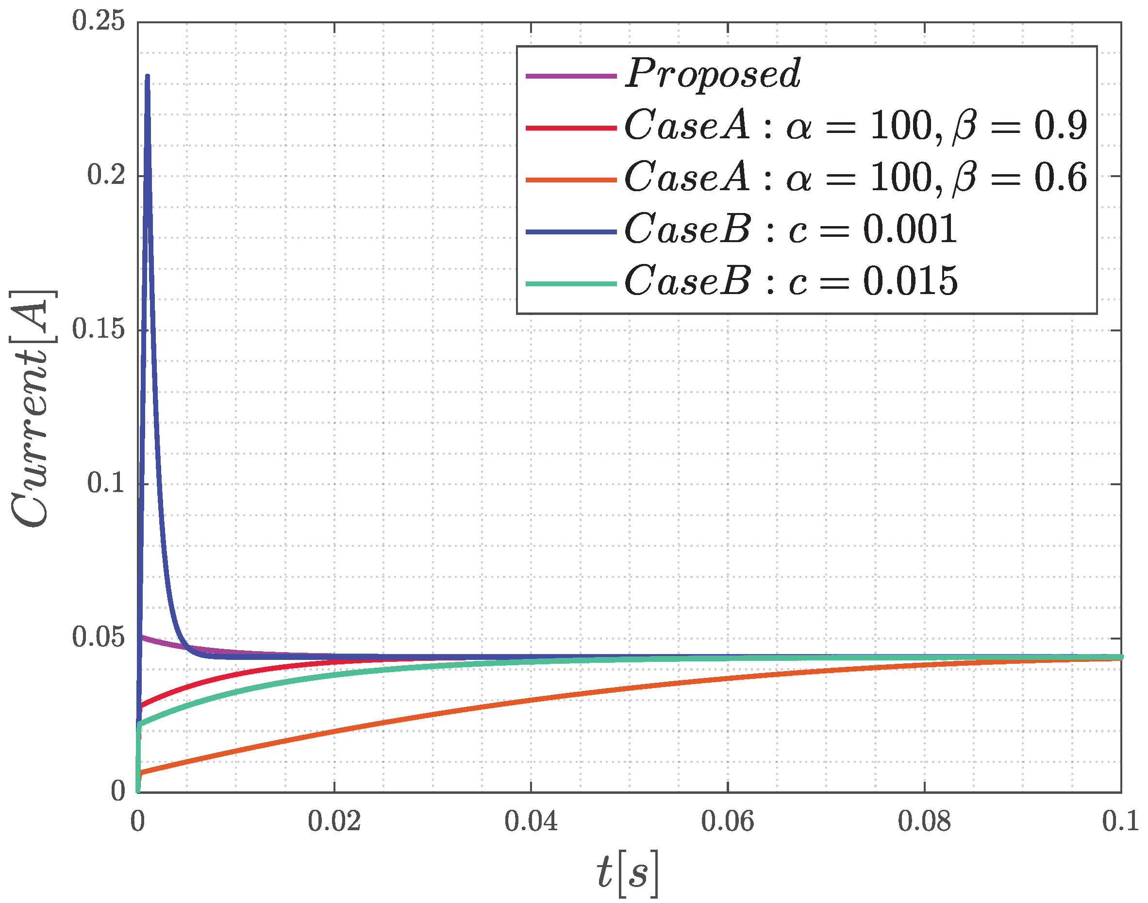
4.2. Discussion of Simulation Results

Figure 2 shows the behavior of the trajectories of the dynamic system in the phase plane, the initial conditions of which are given at the origin. For each case of the sliding surfaces S1 (case A), S2 (case B) and case C (Proposed), one can see that beginning from the initial condition, the states evolve in a different way, until an abrupt change occurs that drives the trajectory to the desired output (3.3 volts). The behavior of the trajectories consist of two stages: when the state trajectory goes to the surface (reaching phase) and when the state trajectory is moving towards the origin along the sliding surface (sliding phase) and exhibits a zig-zag motion. It is clearly seen that the trajectories have a good response—only case B (c = 0.001) does not provide a good response—while the proposed sliding surface (case C) seems to be the best case, as supported by the following simulation results.
Figure 3 shows the finite-time convergence of the sliding variable to zero, for the three sliding surfaces described in Section 2. In this figure, again, one can see that the response provided by case B (c = 0.001) is not as regular as for the other cases, and it is the delayed one, taking more time to reach finite-time convergence. In the figure, one can also see that the proposed surface provides good response and a faster convergence compared to cases A and to case B (c = 0.001). Another analysis is required to verify that the proposed surface provides good response, and this is verified in the following simulation results by plotting the responses of the voltage and current that are associated to the two state variables of the DC–DC buck converter.
The influence of the gain constants and the controller design methodology can be appreciated considering the values given in Table 2, which lists five cases. The simulation response of the different control algorithms is shown in Figure 4 for the voltage behavior, and in Figure 5 for the current behavior. In Figure 4, one can interpret that for the first surface S1 and taking β = 0.6 , the design of the SMC is not sufficiently fast, because the desired value of 3.3 is not reached in 0.1 s, while when β = 0.9 , the response improves significantly, reaching the desired value in 51.2 ms. For the second case S2, by setting c = 0.015 , the desired value is reached in 72.9 ms, while with c = 0.001 , the desired value is reached in 15.2 ms. The proposed sliding surface taken as case C in Section 2 reaches the desired value in 39.4 ms. Another important thing that must be pointed out is that all the responses do not show overshoot behavior—a quality that is related to the gains and the switching control.
The responses shown in Figure 4 for the voltage behavior show that case B (c = 0.001) is the best response. However, taking a look at the results shown in Figure 5 for the current behavior, one can see that the highest overshoot is provided by the sliding surface labeled as case B (c = 0.001), while again, the proposed surface provides a very good response. One can conclude that the surface labeled as case B (c = 0.001) does not provide a good response in the plane, as shown in Figure 2. It does not show a good finite-time convergence, as shown in Figure 3, and it provides the highest current overshoot, as shown in Figure 5. The proposed case C seems to be a good surface for the control of the DC–DC buck converter. However, it is probably possible to find a value between c = 0.001 and c = 0.015 for case B, which would provide a similar transient response both in voltage and current to the proposed case C.
Experimental results on the electronic implementation of some SMC methods can be appreciated in [3,4,6]. In particular, the experimental results given in [6] show that the SMC method suppress the chattering effect and maintains robustness under load variations and parametric uncertainties.

5. Conclusions

This paper showed the application of the SMC method to a DC–DC buck converter. Section 2 summarized three sliding surfaces—two of them already reported and a third one that is introduced in line with the stability analysis given in Section 3. The control strategy was detailed step by step, and it can be seen that the proposed sliding surface takes into consideration not only the voltage error across the capacitor but also the current error through the inductor, which leads to a better control.
The figures showing simulation results in Section 4 provide evidence that the proposed sliding surface is stable and fast, has a good response in the plane (state trajectories), shows a good finite-time convergence and avoids the occurrence of an overshoot in both the voltage across the capacitor and current through the inductor.

Author Contributions

Conceptualization, O.M.-F. and E.T.-C.; methodology, S.H.-M.; software, S.H.-M. and O.M.-F.; formal analysis, S.H.-M. and O.M.-F.; investigation, S.H.-M., O.M.-F. and E.T.-C.; writing—original draft preparation, S.H.-M., O.M.-F. and E.T.-C.; writing—review and editing, S.H.-M., O.M.-F., V.R.G.-D. and E.T.-C.; supervision, V.R.G.-D. and E.T.-C. All authors have read and agreed to the published version of the manuscript.

Funding

This research received no external funding.

Informed Consent Statement

Not applicable.

Data Availability Statement

Not applicable.

Acknowledgments

S.H.-M. thanks to CONACyT-Mexico for the PhD scholarship at INAOE. O.M.-F. thanks to CONACyT-Mexico for the postdoctoral fellowship at INAOE.

Conflicts of Interest

The authors declare no conflict of interest.

Abbreviations

The following abbreviations are used in this manuscript:
MDPIMultidisciplinary Digital Publishing Institute
DOAJDirectory of open access journals
TLAThree letter acronym
LDLinear dichroism

References

  1. Mumtaz, F.; Yahaya, N.Z.; Meraj, S.T.; Singh, B.; Kannan, R.; Ibrahim, O. Review on non-isolated DC-DC converters and their control techniques for renewable energy applications. Ain Shams Eng. J. 2021, 12, 3747–3763. [Google Scholar] [CrossRef]
  2. Warrier, P.; Shah, P. Optimal Fractional PID Controller for Buck Converter Using Cohort Intelligent Algorithm. Appl. Syst. Innov. 2021, 4, 50. [Google Scholar] [CrossRef]
  3. Ullah, N. Fractional order sliding mode control design for a buck converter feeding resistive power loads. Math. Model. Eng. Probl. 2020, 7, 649–658. [Google Scholar] [CrossRef]
  4. Lin, X.; Liu, J.; Liu, F.; Liu, Z.; Gao, Y.; Sun, G. Fractional-order sliding mode approach of buck converters with mismatched disturbances. IEEE Trans. Circuits Syst. Regul. Pap. 2021, 68, 3890–3900. [Google Scholar] [CrossRef]
  5. Sánchez, A.G.S.; Soto-Vega, J.; Tlelo-Cuautle, E.; Rodríguez-Licea, M.A. Fractional-Order Approximation of PID Controller for Buck–Boost Converters. Micromachines 2021, 12, 591. [Google Scholar] [CrossRef] [PubMed]
  6. Kaplan, O.; Bodur, F. Second-order sliding mode controller design of buck converter with constant power load. Int. J. Control 2022, 1–17. [Google Scholar] [CrossRef]
  7. Amin, A.A.; Abdullah, M. A Comparative Study of DC-DC Buck, Boost, and Buck-boost Converters with Proportional-integral, Sliding Mode, and Fuzzy Logic Controllers. Recent Adv. Electr. Electron. Eng. 2022, 15, 75–91. [Google Scholar] [CrossRef]
  8. Belkhier, Y.; Achour, A.; Hamoudi, F.; Ullah, N.; Mendil, B. Robust energy-based nonlinear observer and voltage control for grid-connected permanent magnet synchronous generator in the tidal energy conversion system. Int. J. Energy Res. 2021, 45, 13250–13268. [Google Scholar] [CrossRef]
  9. Al Alahmadi, A.A.; Belkhier, Y.; Ullah, N.; Abeida, H.; Soliman, M.S.; Khraisat, Y.S.H.; Alharbi, Y.M. Hybrid wind/PV/battery energy management-based intelligent non-integer control for smart DC-microgrid of smart university. IEEE Access 2021, 9, 98948–98961. [Google Scholar] [CrossRef]
  10. Kaleem, A.; Khalil, I.U.; Aslam, S.; Ullah, N.; Al Otaibi, S.; Algethami, M. Feedback PID Controller-Based Closed-Loop Fast Charging of Lithium-Ion Batteries Using Constant-Temperature–Constant-Voltage Method. Electronics 2021, 10, 2872. [Google Scholar] [CrossRef]
  11. Sami, I.; Ullah, S.; Ali, Z.; Ullah, N.; Ro, J.S. A super twisting fractional order terminal sliding mode control for DFIG-based wind energy conversion system. Energies 2020, 13, 2158. [Google Scholar] [CrossRef]
  12. Belkhier, Y.; Achour, A.; Shaw, R.N.; Ullah, N.; Chowdhury, M.S.; Techato, K. Energy-based combined nonlinear observer and voltage controller for a PMSG using fuzzy supervisor high order sliding mode in a marine current power system. Sustainability 2021, 13, 3737. [Google Scholar] [CrossRef]
  13. Chafekar, N.; Mate, U.; Kurode, S.; Vyawahare, V. Design and implementation of fractional order sliding mode controller for DC-DC Buck Converter. In Proceedings of the 2019 Fifth Indian Control Conference (ICC), New Delhi, India, 9–11 January 2019; pp. 201–206. [Google Scholar]
  14. Yang, N.; Wu, C.; Jia, R.; Liu, C. Fractional-order terminal sliding-mode control for buck DC/DC converter. Math. Probl. Eng. 2016, 2016. [Google Scholar] [CrossRef] [Green Version]
  15. Xie, L.; Liu, Z.; Ning, K.; Qin, R. Fractional-Order Adaptive Sliding Mode Control for Fractional-Order Buck-Boost Converters. J. Electr. Eng. Technol. 2022, 17, 1693–1704. [Google Scholar] [CrossRef]
  16. Taheri, B.; Sedaghat, M.; Bagherpour, M.A.; Farhadi, P. A New Controller for DC-DC Converters Based on Sliding Mode Control Techniques. J. Control Autom. Electr. Syst. 2019, 30, 63–74. [Google Scholar] [CrossRef]
  17. Ali, S.; Raza, M.T.; Abbas, G.; Ullah, N.; Al Otaibi, S.; Luo, H. Sliding Mode Observer-Based Fault Detection in Continuous Time Linear Switched Systems. Energies 2022, 15, 1090. [Google Scholar] [CrossRef]
  18. Utkin, V.; Guldner, J.; Shi, J. Sliding Mode Control in Electro-Mechanical Systems; CRC Press: Boca Raton, FL, USA, 2017. [Google Scholar]
  19. Khalil, H.K. Nonlinear Control; Pearson: New York, NY, USA, 2015; Volume 406. [Google Scholar]
  20. Labbadi, M.; Cherkaoui, M. Robust adaptive nonsingular fast terminal sliding-mode tracking control for an uncertain quadrotor UAV subjected to disturbances. ISA Trans. 2020, 99, 290–304. [Google Scholar] [CrossRef] [PubMed]
  21. Shtessel, Y.; Edwards, C.; Fridman, L.; Levant, A. Sliding Mode Control and Observation; Springer: Berlin/Heidelberg, Germany, 2014; Volume 10. [Google Scholar]
Figure 1. Generic DC–DC buck converter topology.
Technologies 11 00033 g001
Figure 2. Phase portraits of the three sliding surfaces given in Section 2.
Technologies 11 00033 g002
Figure 3. Finite-time convergence of the sliding surfaces to the output variable for the cases given in Section 2.
Technologies 11 00033 g003
Figure 4. Voltage responses of the SMC for the three sliding surfaces described in Section 2.
Technologies 11 00033 g004
Figure 5. Current responses of the SMC for the three sliding surfaces described in Section 2.
Technologies 11 00033 g005
Table 1. Parameter values.
DescriptionParameterValueUnits
InductorL0.02H
CapacitorC10 4 F
Load resistanceR75 Ω
Input voltageE5V
Reference voltageV_d3.3V
Table 2. Surface gains and constant values for the three cases.
SurfaceGain
case A α = 100 , β = 0.9 , K = 1
case A α = 100 , β = 0.6 , K = 1
case Bc = 0.001, K = 1
case Bc = 0.015, K = 1
case C (Proposed) α = 500 , β = 1
Disclaimer/Publisher’s Note: The statements, opinions and data contained in all publications are solely those of the individual author(s) and contributor(s) and not of MDPI and/or the editor(s). MDPI and/or the editor(s) disclaim responsibility for any injury to people or property resulting from any ideas, methods, instructions or products referred to in the content.

