Article

A Stochastically Correlated Bivariate Square-Root Model

by
Allan Jonathan da Silva
1,2,*,
Jack Baczynski
1 and
José Valentim Machado Vicente
3
1
Coordination of Mathematical and Computational Methods, National Laboratory for Scientific Computing (LNCC), Petrópolis 25651-075, RJ, Brazil
2
Department of Production Engineering, Federal Center for Technological Education (CEFET/RJ), Itaguaí 23812-101, RJ, Brazil
3
Institute of Mathematics and Statistics, Rio de Janeiro State University (UERJ), Rio de Janeiro 20550-900, RJ, Brazil
*
Author to whom correspondence should be addressed.
Int. J. Financial Stud. 2024, 12(2), 31; https://doi.org/10.3390/ijfs12020031
Submission received: 30 January 2024 / Revised: 18 March 2024 / Accepted: 20 March 2024 / Published: 25 March 2024

Abstract

:
We introduce a novel stochastically correlated two-factor (i.e., bivariate) diffusion process under the square-root format, for which we analytically obtain the corresponding solutions for the conditional moment-generating functions and conditional characteristic functions. Such solutions recover verbatim those of the uncorrelated case which encompasses a range of processes similar to those produced by a bivariate square-root process in which entries are correlated in the standard way, that is, via a constant correlation coefficient. Note that closed-form solutions for the conditional characteristic and moment-generating functions are not available for the latter. We focus on the financial scenario of obtaining closed-form expressions for the exact price of a zero-coupon bond and Asian option prices using a Fourier cosine series method.

1. Introduction

1.1. Motivation

Scalar square-root diffusion processes, also called CIR processes, due to Cox et al. (1986), have two properties that are important in applications in finance: (i) they ensure mean reversion of the state variables towards a long-run level and (ii) unlike the Vasicek (1977) model, they do not take negative values. The importance of such properties clearly replicates in the multi-dimensional scenario, especially when correlation is allowed among the the process entries.
In turn, stochastic models found in finance, especially in interest rate markets, usually assume uncorrelated state variables that contradict both intuition and historical data. In fact, considerable difficulties arise in the pricing procedures when entering correlation in the model, even when numerical solutions of the corresponding partial differential equations are given by finite difference or finite element methods. Concerning this matter, we quote Brigo and Mercurio (2006): “requiring d W 1 d W 2 = ρ d t with ρ 0 in the two-factor CIR model would indeed destroy analytical tractability: It would no longer be possible to compute bond prices and rates analytically starting from the short rate factors.” On the other hand, as argued by Brigo and Mercurio (2006), whenever the correlation plays a more relevant role or when higher precision is needed in the pricing procedure, we need to resort to models that allow for more realistic patterns.
Developing an analytical solution for the moment-generating and characteristic functions of a two-factor CIR model with stochastic correlation is essential for accurately pricing financial derivatives and managing risk in markets where interest rates are governed by two stochastic interdependent factors. This requires solving a partial differential equation that accounts for the dynamic interplay between the two factors under a stochastic correlation. Achieving this would significantly enhance our comprehension of and capacity to forecast the behavior of financial instruments in a more integrated and realistic manner, reflecting the inherent linkages in interest rate markets.
The central research question guiding this study is how to incorporate stochastic correlation into a bivariate square-root model, thereby improving the pricing of interest rate derivatives influenced by the two interdependent stochastic factors.

1.2. Contribution

In this study, we present a bi-dimensional (two-factor) mean reversion stochastically correlated process in which entries are produced by two concatenated CIR-type models (Cox et al. 1986). This process is affine according to Duffie and Singleton (2003).
We obtained the closed-form solution—of the exponential format—of the conditional moment-generating function and the conditional characteristic function of the density function of the integral of the process governed by the model as well as those of the process itself at the final time T. The key point that permitted us to apply the above transforms to the problem of pricing derivatives, particularly with respect to fixed income markets, was that the integral of the process—and not the process per se—was an adequate mathematical object to achieve the results.
It is noteworthy that by setting our stochastic correlation to zero, we reduced our model to a pair of scalar uncorrelated square-root diffusions. We believe that the proposed model encompasses a range of processes similar to those produced by a bivariate CIR process in which entries are correlated in the standard way, that is, exhibiting a constant correlation coefficient, with the advantage of exhibiting an analytical solution.
We applied our results in the context of interest rate financial markets where the interest rate process stems from the two-factor stochastically correlated CIR model presented in this paper. We obtained closed-form expressions for the price of a zero-coupon bond and, in the following, for the price of the IDI option, an Asian option that commonly appears in Brazilian fixed-income markets. For the latter case, we used the fast and accurate pricing method based on the Fourier series expansions proposed by Fang and Oosterlee (2008) and applied it to interest rate options as in da Silva et al. (2019).
Via numerical simulations, we showed the (good) behavior of the two-factor process in the face of a certain stochastic correlation condition, under stringent circumstances. Moreover, a result concerning the effect of the sensitivity parameter ( ϵ ) on the stochastic correlation coefficient ( ϱ ), and ultimately, the possibility of emulating bivariate CIR processes with a constant correlation coefficient, was unveiled. Focusing on the financial scenario, we analyzed the impact of the correlation parameter ( ρ ) on the conditional probability density functions associated with the interest rate process—which in turn stems from the two-factor process—again obtaining a good confirmation (non-negativity). In addition, option price curves were obtained and parameterized by ρ . We also used real financial market data for the model design. Finally, to address model performance, we calibrated the model to the term structure of interest rates. We compared the uncorrelated CIR model, stochastically correlated model, and stochastically correlated model with jumps.
The mathematical tools we relied on were the Feynman–Kac formula explained by Oksendal (2007), the separation of variables approach found in Duffie (2001), the Riccati equations (Reid 1972) with known explicit solutions with step-by-step solutions shown by Bouziane (2008), and the series expansions proposed by Fang and Oosterlee (2008).

1.3. Paper Outline

The remainder of this paper is organized as follows: Related works are presented in Section 2. Section 3 presents the stochastically correlated two-factor affine model and its probability background. In Section 4, we derive the expressions for the conditional moment-generating function and conditional characteristic function associated with the model. Section 5 addresses applications to finance, and Section 6 presents the numerical results. Finally, Section 7 concludes the paper.

2. Literature Review

Stochastic correlation models in financial markets have garnered significant interest for their implications for risk management and derivative pricing. L. Márkus and Kumar (2019) established the main required properties such as (i) taking values between ( 1 , 1 ) , (ii) varying around a constant mean value in the mean-reverting sense, and (iii) having a probability mass tending to zero at the boundaries. L. Márkus and Kumar (2019) compared five stochastic correlation models typically found in the literature. Kim and Jo (2014) proposed a correlated stochastic process, highlighting its inherent scale invariance and convergence properties, which are crucial for financial data analysis. Concurrently, Leippold and Trojani (2010)’s research on matrix affine jump diffusions introduces a comprehensive framework for assessing multivariate financial risks, such as jumps in the correlation structure, emphasizing the versatility and depth of their approach. Teng et al. (2017) further contribute to this discourse by scrutinizing stochastic correlations within the context of European-style Quanto options pricing, revealing the limitations of the traditional constant correlation assumptions.
Complementing these studies, Márkus and Kumar (2021) investigated the stochastic correlation between asset prices by employing innovative goodness-of-fit procedures that underscore the complexities of asset price interdependence. This body of work collectively advances our understanding of stochastic correlations, offering nuanced insights into their practical applications and theoretical underpinnings in financial modeling. Luo and Seco (2017) compared forecasting performance using a set of models to evaluate stochastic correlation. In the realm of fixed-income products, Stehlíková (2020) finds a partial differential equation solution for bond prices using a series expansion for the stochastic correlation term.
More recently, Kim et al. (2023) developed a multi-asset option pricing model applied to the Quanto option. The authors assumed that asset processes follow a normal tempered stable process with the Ornstein–Uhlenbeck stochastic correlation process. The authors demonstrated that the model is justified by empirical results.

3. The Model

Let ( Ω , F , Q , { F t } t [ 0 , T ] ) be a filtered space, where { F t } t [ 0 , T ] is a filtration, Q is a probability measure, and the adapted processes Z 1 = ( Z 1 ( t ) , t [ 0 , T ] ) and Z 2 = ( Z 2 ( t ) , t [ 0 , T ] ) are independent standard Brownian Motions under Q (see, e.g., Protter (2005)).
We introduce a pair of square-root diffusions (Cox et al. 1986), in which the underlying variables are stochastically correlated, as follows. For t [ 0 , T ] and the initial conditions x 1 ( 0 ) = x ¯ 1 and x 2 ( 0 ) = x ¯ 2 ,
d x 1 ( t ) = κ 1 ( θ 1 x 1 ( t ) ) d t + σ 1 x 1 ( t ) d W 1 ( t )
and
d x 2 ( t ) = κ 2 ( θ 2 x 2 ( t ) ) d t + σ 2 ( 1 ρ 2 ) x 2 ( t ) d W 2 ( t ) ,
where x ¯ 1 > 0 and x ¯ 2 > 0 are prescribed random variables and ρ [ 0 , 1 ) is the correlation coefficient. We have that κ i , θ i , and σ i are positive real numbers. Each stochastic process x i ( t ) is pulled to a mean level θ i at a rate κ i with volatility parameter σ i . We have that W 1 and W 2 are stochastically correlated processes, where W 1 ( t ) = Z 1 ( t ) is a Brownian Motion and
W 2 ( t ) = 0 t ϱ ( t ) d Z 1 ( t ) + 0 t 1 ϱ ( t ) 2 d Z 2 ( t )
is an Itô process (Oksendal 2007).
Hence, according to Musiela and Rutkowski (1998),
d [ W 1 , W 1 ] ( t ) = d [ W 2 , W 2 ] ( t ) = d t , and d [ W 1 , W 2 ] ( t ) = ϱ ( t ) d t .
The correlation ϱ is specified via the adapted stochastic process
ϱ ( t ) = ρ ϵ x 1 ( t ) x 2 ( t ) ( 1 ρ 2 ) ,
ρ ( 1 , 1 ) . Note that if ρ = 0 , then W 2 = Z 2 and we recover the standard uncorrelated case. If we change the specification of ϱ to a constant, say, ϱ = ρ , then W 2 = ρ Z 1 + 1 ρ 2 ) Z 2 and E [ W 2 2 ( t ) ] = t , and so W 2 becomes a standard Brownian Motion.
The dynamics in (1) and (2) also reads
d x 1 ( t ) d x 2 ( t ) = κ 1 ( θ 1 x 1 ( t ) ) κ 2 ( θ 2 x 2 ( t ) ) d t + σ ¯ ( x 1 ( t ) , x 2 ( t ) ) d Z 1 ( t ) d Z 2 ( t ) ,
where
σ ¯ ( x 1 ( t ) , x 2 ( t ) ) = σ 1 x 1 ( t ) 0 0 σ 2 ( 1 ρ 2 ) x 2 ( t ) 1 0 ϱ ( t ) 1 ( ϱ ( t ) ) 2
and Z 1 and Z 2 are independent standard Brownian Motions, as defined at the beginning of the section. Using specification (5) and some algebraic manipulation, it follows that σ ¯ ( x 1 ( t ) , x 2 ( t ) ) σ ¯ ( x 1 ( t ) , x 2 ( t ) ) is of affine form (Duffie 2001).
In the above equations, κ i are the speeds of adjustment, θ i are the long-term means, σ i are the volatility factors, ρ is a correlation parameter, and ϵ is a sensitivity factor—a useful parameter as we shall see in Section 6. Equations (1) and (2) produce the Feller processes known in the context of finance as the CIR processes due to Cox et al. (1986). According to Bertini and Passalacqua (2008), the following condition must hold to ensure a strong solution for (1) and (2) and to avoid the possibility of negative values of x 1 and x 2 .
2 κ 1 θ 1 σ 1 2 + 2 κ 2 θ 2 σ 2 2 ( 1 ρ 2 ) 1 .
Moreover, we rely on having
ϱ ( t ) 2 1 a . s . t [ 0 , T ] .
To conform with the condition above, we benefit from the existence of the sensitivity parameter ϵ , setting it as follows.
ϵ 0 , ( 1 ρ 2 ) m i n ( x ¯ 1 , θ 1 ) m i n ( x ¯ 2 , θ 2 ) .
The comprehensive numerical results in Section 6 assert that the above condition suffices to ensure the good behavior of the correlation process and that the bivariate process x covers a broad range of CIR-type correlated processes.

4. Underpinning Results

The following theorems consider the stochastically correlated two-factor process x ( t ) = ( x 1 ( t ) , x 2 ( t ) ) , as given by the system in Equation (6), relying on the fact that this process is affine in the sense of Duffie (2001). Here, the symbol ’ stands for the transpose.
The moment-generating function (MGF) of a random variable X is defined as the expected value of the exponential function of t X , where t is a real-valued parameter (Ross 2007). Mathematically, the MGF M X ( t ) of a random variable X is given by:
M X ( t ) = E ( e t X )
The MGF provides a systematic way to compute the moments of a distribution, such as the mean, variance, skewness, and kurtosis, by taking derivatives of the MGF with respect to t and evaluating them at t = 0 .
Conversely, the characteristic function of a random variable X is defined as the expected value of the complex exponential function of i t X , where i is the imaginary unit and t is a real-valued parameter. Mathematically, the characteristic function ϕ X ( t ) of a random variable X is given by:
ϕ X ( t ) = E ( e i t X )
Similar to MGF, the characteristic function provides a way to fully describe the distribution of a random variable. It contains all information about the distribution, allowing for the computation of moments and other statistical properties.
The conditional moment-generating function and the characteristic function of Theorem 1 are applied in Section 5 to calculate the price of a zero-coupon bond and the price of an interest rate option, namely, the IDI option. In both cases, the interest rate is given by the additive process η 1 x 1 ( t ) + η 2 x 2 ( t ) , which stems from the two-factor process x.
Theorem 1.
The closed-form solution of the conditional characteristic function (resp. conditional moment-generating function) associated with the [ t , T ] -integral of the two-factor process x with coefficient η = ( η 1 , η 2 ) R 2 , namely, t T η x ( s ) d s (resp. t T η x ( s ) d s ), is given by
f ^ ( x ( t ) , t , u ) = E [ e i u t T η x ( s ) d s x ( t ) ] = e α ( t , T ) β 1 ( t , T ) x 1 ( t ) β 2 ( t , T ) x 2 ( t )
resp . G ( x ( t ) , t , u ) = E [ e u t T η x ( s ) d s x ( t ) ] = e α ( t , T ) β 1 ( t , T ) x 1 ( t ) β 2 ( t , T ) x 2 ( t )
where
α ( t , T ) = t T κ 1 θ 1 β 1 ( t , T ) κ 2 θ 2 β 2 ( t , T ) + ρ ϵ σ 1 σ 2 β 1 ( t , T ) β 2 ( t , T ) d s ,
β j ( t , T ) = 2 η j e γ j ( T t ) 1 ( γ j + κ j ) e γ j ( T t ) + ( γ j κ j ) , j = 1 , 2 ,
with
γ 1 = κ 1 2 + 2 i σ 1 u η 1 a n d γ 2 = κ 2 2 + 2 i σ 2 ( 1 ρ 2 ) u η 2
( r e s p . γ 1 = κ 1 2 + 2 σ 1 u η 1 a n d γ 2 = κ 2 2 + 2 σ 2 ( 1 ρ 2 ) u η 2 ) .
Proof. 
We address the proof of the moment-generating function. The proof for the characteristic function case closely follows. Therefore, invoking Duffie and Singleton (2003), the moment-generating function of a multifactor equation—say, an m-dimensional, stochastic differential equation (SDE) of the form
d x ( t ) = μ ( x ( t ) ) d t + σ ( x ( t ) ) d W ( t ) ,
—has an exponential affine solution if the above coefficients are of the form
μ ( x ) = K 0 + K 1 x and ( σ ( x ) σ ( x ) ) i j = H 0 i j + H 1 i j x ,
where K 0 , K 1 , H 0 i j , and H 1 i j have adequate dimensions and do not depend on x.
The above SDE captures (1) and (2), setting m = 2 , K 0 = [ κ 1 θ 1 ; κ 2 θ 2 ] , K 1 = κ 1 0 0 κ 2 , and
( σ ( x ) σ ( x ) ) = σ 1 2 x 1 ρ σ 1 σ 2 ϵ ρ σ 1 σ 2 ϵ σ 2 2 ( 1 ρ 2 ) x 2 ,
that is, the coefficients are of the affine form. To obtain det ( σ ( x ) σ ( x ) ) > 0 , we require
x 1 x 2 ( 1 ρ 2 ) > ρ 2 ϵ 2 .
Applying the Feynman–Kac formula (Oksendal 2007) to the second expression of (12), we obtain
G ( x ( t ) , t , u ) t + G ( x ( t ) , t , u ) ( K 0 + K 1 x ) + i , j G ( x ( t ) , t , u ) x i x j ( H 0 i j + H 1 i j x ) = u η x G ( x ( t ) , t , u ) .
Therefore, invoking the last expression of Equation (11), we have:
α t + x 1 ( t ) β 1 t + x 2 ( t ) β 2 t + [ κ 1 ( θ 1 x 1 ( t ) ) ] β 1 + [ κ 2 ( θ 2 x 2 ( t ) ) ] β 2 + 1 2 σ 1 2 x 1 ( t ) β 1 2 + 1 2 σ 2 2 x 2 ( t ) β 2 2 ( 1 ρ 2 ) + ρ σ 1 σ 2 β 1 β 2 ϵ = u η x ( t ) .
Gathering the terms in x 1 and x 2 gives us
α t = κ 1 θ 1 β 1 κ 2 θ 2 β 2 ρ σ 1 σ 2 β 1 β 2 ϵ
and the Riccati differential equations
β 1 t = κ 1 β 1 σ 1 2 2 β 1 2 + η 1
and
β 2 t = κ 2 β 2 σ 2 2 2 β 2 2 ( 1 ρ 2 ) + η 2 .
Now, for terminal conditions, we have
α ( T , T ) = β 1 ( T , T ) = β 2 ( T , T ) = 0
After some algebraic manipulation, we obtain that the solutions of Riccati Equations (20) and (21) are given by Equations (13) and (14). □
The characteristic function version of the following theorem is applied in Section 6 to calculate the probability density function of the additive process η 1 x 1 ( t ) + η 2 x 2 ( t ) .
Theorem 2.
The closed-form solution of the conditional characteristic function associated with the two-factor process x at time T with coefficient η = ( η 1 , η 2 ) R 2 , namely, η x T , is given by
f ^ ( x ( t ) , t , u ) = E [ e i u η x ( T ) x ( t ) ] = e ( α ( t , T ) β 1 ( t , T ) x 1 ( t ) β 2 ( t , T ) x 2 ( t ) ) ,
where
α ( t , T ) = t T κ 1 θ 1 β 1 ( s ) κ 2 θ 2 β 2 ( s ) + ρ ϵ σ 1 σ 2 β 1 ( s ) β 2 ( s ) d s ,
β 1 ( t , T ) = 2 κ 1 e κ 1 t i u η σ 1 2 ( e κ 1 t 1 ) i u η 2 κ 1 ,
β 2 ( t , T ) = 2 κ 2 e κ 2 t i u η σ 2 2 ( 1 ρ 2 ) ( e κ 2 t 1 ) i u η 2 κ 2 .
Proof. 
Following the same steps as those in the proof of Theorem 1, we obtain the Riccati differential equations
β 1 t = κ 1 β 1 σ 1 2 2 β 1 2
and
β 2 t = κ 2 β 2 σ 2 2 2 β 2 2 ( 1 ρ 2 ) ,
and are given the terminal conditions
α ( T , T ) = 0 , and β 1 ( T , T ) = i u η 1 , and β 2 ( T , T ) = i u η 2 ,
Again, after some algebraic manipulation, we obtain Equations (24) and (25), respectively, satisfying Riccati Equations (26) and (27).□
A comprehensive step-by-step solution to the partial differential equations of the affine jump diffusion models can be found in Bouziane (2008).
Remark 1.
It is worth mentioning that the two-factor uncorrelated CIR process given by
d x 1 ( t ) = κ x ( θ 1 x 1 ( t ) ) d t + σ 1 x 1 ( t ) d W 1 ( t ) ,
d x 2 ( t ) = κ r ( θ 2 x 2 ( t ) ) d t + σ 2 x 2 ( t ) d W 2 ( t ) ,
introduced in the famous paper by Cox et al. (1986), in which a closed-form solution is shown in the work of Brigo and Mercurio (2006), is a particular case of the analytical solution (11) with ρ = 0 .

5. Applications to Finance: Fixed-Income Markets with Decomposed Nominal Rates

We consider a financial interest rate market underpinned by the short rate stochastic process R = ( R ( t ) , t [ 0 , T ] ) which stems from the two-factor stochastically correlated (affine) CIR model given by (1)–(4), namely,
R ( t ) = η 1 x 1 ( t ) + η 2 x 2 ( t ) ,
( η 1 , η 2 ) R 2 . We assume that Q is a risk-neutral probability measure.
Recalling the Fisher effect (Fisher 1930) in economics, we have that the nominal short rate R ( t ) can be decomposed into the real interest rate and inflation expectation. This conforms to our setting, simply particularizing ( η 1 , η 2 ) = ( 1 , 1 ) and denoting, for convenience, the real interest rate and inflation by x 1 ( t ) and x 2 ( t ) , respectively.
Under this framework, and relying on Theorem 1, we obtain the price of a bond and an interest rate option as follows:

Bond Pricing

The zero-coupon bond is an interest rate derivative that pays 1 at the expiration date T and no other payment before T. Relying on the seminal work of Harrison and Pliska (1981), the no-arbitrage price at time t [ 0 , T ] of the zero-coupon bond expiring at T is given by
D ( t , T ) = E Q e t T R ( s ) d s | R ( t ) .
Proposition 1.
Consider an interest rate market with nominal short rate given by Equation (30), ( η 1 , η 2 ) = ( 1 , 1 ) , where the real yield x 1 ( t ) and inflation premium x 2 ( t ) follow the stochastically correlated square-root diffusion model (1)–(4). Then, the dynamic of the no-arbitrage price of the bond at time interval [ 0 , T ] is given by
d D ( t , T ) = D ( t , T ) { η 1 x 1 ( t ) + η 2 x 2 ( t ) d t + σ 1 β 1 ( t , T ) d W 1 Q ( t ) + σ 2 ( 1 ρ 2 ) β 2 ( t , T ) d W 2 Q ( t ) } .
Proof. 
Using the moment-generating function version of Theorem 1, we have that the solution to Equation (31) is of the exponential affine form, as given by the right side of (11) with ( η 1 , η 2 ) = ( 1 , 1 ) . Relying on Ito’s formula and after some algebraic manipulation, it follows that
d D ( t , T ) = D ( t , T ) [ α t ( t , T ) + β 1 ( t , T ) x 1 ( t ) + β 2 ( t , T ) x 2 ( t ) κ 1 ( θ 1 x 1 ( t ) ) β 1 ( t , T ) κ 2 ( θ 2 x 2 ( t ) ) β 2 ( t , T ) + + 1 2 σ 1 2 x 1 ( t ) β 1 ( t , T ) 2 + 1 2 σ 2 2 ( 1 ρ 2 ) x 2 ( t ) β 2 ( t , T ) 2 + σ 1 σ 2 ρ ϵ β 1 ( t , T ) β 2 ( t , T ) ] d t + + D ( t , T ) σ 1 β 1 ( t , T ) d W 1 Q ( t ) + σ 2 ( 1 ρ 2 ) β 2 ( t , T ) d W 2 Q ( t ) .
Using Equations (20) and (21) for β 1 ( t , T ) and β 2 ( t , T ) , respectively, we obtain Equation (32). □
We may notice that the drift that ultimately appears in dynamic (32) is the short rate process itself, as it should be.
As stated by Brigo and Mercurio (2006) and shown in the work of Jamshidian and Zhu (1997), for example, a two-factor model can explain up to 91 % of the variations in the yield curve. Such a model is required to provide a realistic evolution of the zero-coupon bond curve. Therefore, we contribute to this by sophisticating the modeling of the term structure of interest rates via the additive two-factor model given by (1)–(4), (30), and ( η 1 , η 2 ) = ( 1 , 1 ) . We also provide a leak concerning the statement made by Brigo and Mercurio (2006), in which the authors say that “requiring d W 1 d W 2 = ρ d t with ρ 0 in the two-factor CIR model would indeed destroy analytical tractability: It would no longer be possible to analytically compute bond prices and rates starting from the short rate factors.” Indeed, we have shown that bond prices are analytically tractable under the two-factor correlated CIR model.

6. Numerical Results

In this section, we discuss some issues of the stochastically correlated square-root diffusion process given by Equations (1)–(4). In Section 6.1, we study the model’s behavior in the face of the condition given by the inequality (9)—which involves the stochastic correlation coefficient ϱ . In Section 6.2, we study the variation in the stochastic correlation coefficient ϱ in time and in probability space for fixed parameters ρ and ε . In the following, we let these parameters vary.
Using the Fourier series, in Section 6.3, we present the conditional probability density function of the integral of the short-rate process R—the weighted sum of the components of the two-factor CIR model (1)–(4) (see Equation (30)). The conditional probability density function is provided equally for R at terminal date T. This conditional density function is the cornerstone of obtaining the price of financial derivative contracts. We shall see that, in the long run, the correlation parameter ρ plays a sensitive role in the volatility of the zero-coupon bond and, therefore, on the prices of the interest rate derivatives. In the following section, we obtain the price of the IDI option (Section 6.4). Section 6.4 presents the calibration results for the term structure of interest rates.
Nonetheless, the important stochastic correlation analysis will be carried out varying ϵ in the whole range given by (34). Our dynamic is as given by Equations (1)–(4) with κ 1 = 0.15 , κ 2 = 0.15 , θ 1 = 0.05 , θ 2 = 0.05 , σ 1 = 0.015 , σ 2 = 0.025 , T t = 1 year, and initial condition x 1 ( 0 ) = 0.05 and x 2 ( 0 ) = 0.05 . We also set η 1 = η 2 = 1 . We benefit from the existence of the sensitivity parameter ϵ , setting it equal to the maximal value of the range given by (10), that is,
ϵ = ( 1 ρ 2 ) min ( x 1 ( 0 ) , θ 1 ) min ( x 2 ( 0 ) , θ 2 ) .
This maximum value is maintained throughout this section. Nonetheless, the important stochastic correlation analysis will be carried out varying ϵ in the whole range given by (10).
Figure 1 illustrates a bivariate sample path evolving according to (1)–(4), with ρ = 0.5 and ϵ as above.

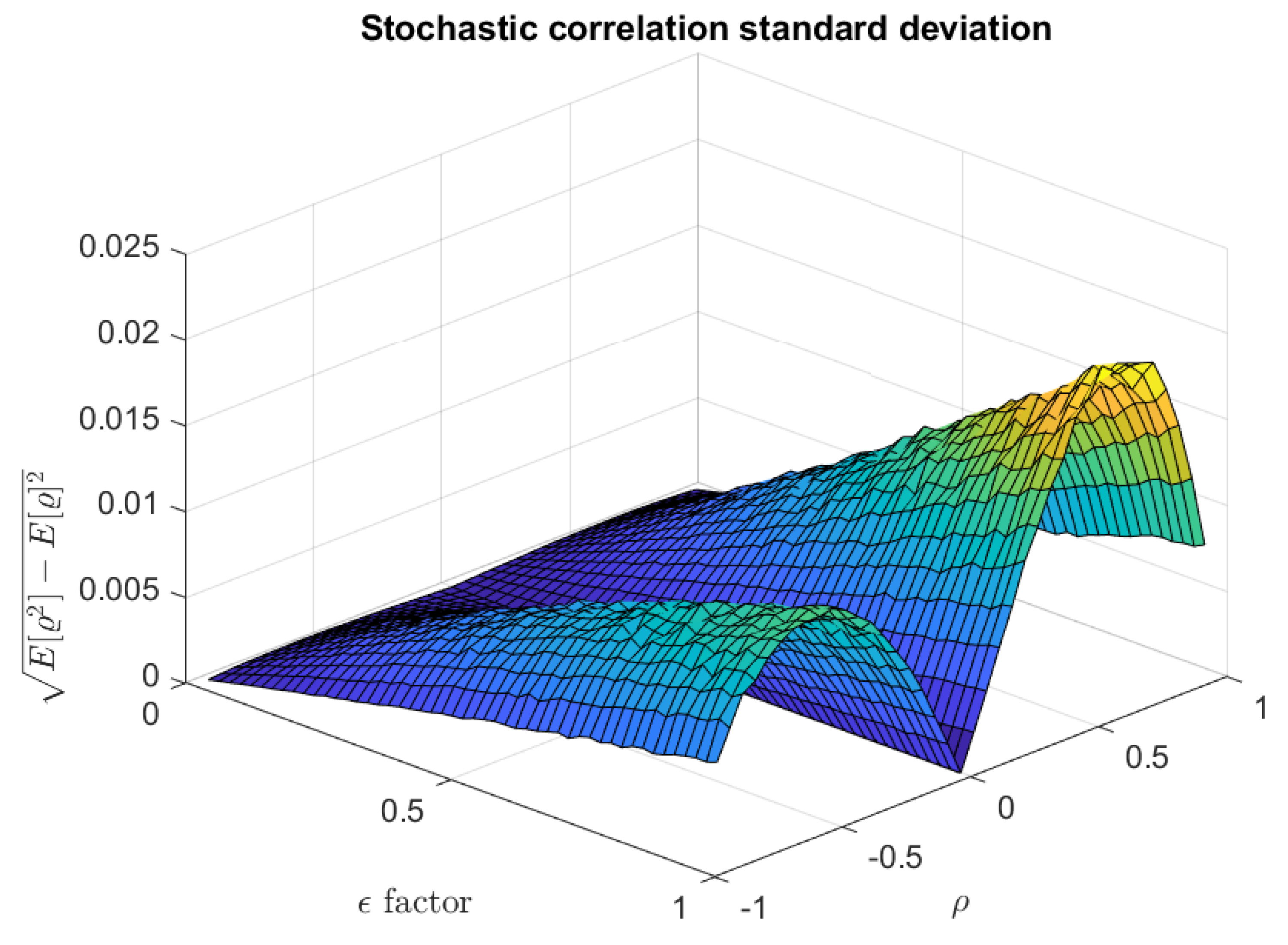
6.1. The Stochastic Correlation Condition (9) Is Mild, at Least at a Certain Niche

To verify whether the stochastic correlation coefficient ϱ ( t ) performs according to condition (9), we produced 100.000 path simulations of the stochastically correlated CIR process with time discretization Δ t = 0.01 years and a period of one year, using the simple Euler scheme as given in the work of Glasserman (2004).
First, we used the work of Almeida and Vicente (2009), who provided us with parameter estimates based on real-world financial data. The authors used a three-factor uncorrelated CIR process to model zero-coupon bonds. We tested all three possible combinations of the parameters of the referenced paper, as shown in Table 1, and did not find a rate of over 0.01 % concerning pointwise violations of the stochastic correlation condition (9) throughout [ t , T ] , for the various values of ρ .
To test a more restrictive scenario, we set κ 1 = κ 2 = 0.75 , θ 1 = θ 2 = 0.01 , and σ 1 = σ 2 = 0.03 for x 1 ( t ) = θ 1 and x 2 ( t ) = θ 2 . In agreement with condition (8), the setup above forces the model to violate the stochastic correlation condition. However, in the beginning, no violation of this condition occurred for a variety of values of ρ . Violations begin to appear when σ 1 , 2 reaches 0.05 . Nevertheless, the rate did not exceed 9 % for a reasonably broad range of σ 1 , 2 , typically up to 0.1 . Hence, this shows that condition (9) is in fact mild, at least for ϵ prescribed as in (34). In addition, we noticed that the violation rate decreased with the correlation parameter ρ .

6.2. Hand-Conducting the Model via ϵ

Figure 2 shows a sample path ϱ ( t , ω ) of the stochastic correlation coefficient given by (5). It suggests that ϱ has little variation over time. In addition, from the simulations, we could infer that, for any ρ , 99 % of the sample paths lay within the range of ± 0.10 .
Therefore, we may infer that our model can be a good approximation of correlated CIR models with a constant correlation coefficient, with the advantage of exhibiting an analytical pricing solution.
Now, for each ρ [ 1 , + 1 ] and for ϵ prescribed by the relation (34), Figure 3 exhibits the mean value over time of a corresponding sample path ϱ of the stochastic correlation coefficient. Since ϱ does not vary much either in time or in space, we shall rename this mean value as the operation point of the stochastic correlation coefficient, for each ρ .
As shown in Figure 3, this operation point covers the interval [ 0.5 , + 0.5 ] , which is not very broad but still a reasonable range as we vary ρ . Alternatively, we can depart from the maximum value of ϵ given by inequality (34) to an arbitrary value in a certain confidence interval, so we can hand-conduct the curve of operation points to another more desired range.
Figure 4 shows the stochastic correlation mean surface for ϵ varying in the range given by (10), and Figure 5 shows the corresponding standard deviation. These two graphs illustrate some important findings. Firstly, for every ρ in ( 1 , 1 ) , the following hold:
  • The correlation mean vanishes when ϵ 0 (see Figure 4).
  • The correlation stochasticity also vanishes when ϵ 0 (see Figure 5).
In addition, the model recasts the specific case of an uncorrelated CIR model when either ρ = 0 or ϵ = 0 , for any given parameter values.
Second, while not near the degenerated zero value, ϵ indeed introduces a correlation between the entries of the process generated by the model, whose intensity varies considerably as we hand-conduct it within the range established in (10).
These qualities underscore the versatility of the model in capturing a range of behaviors, including scenarios that are essential for theoretical analysis and practical applications.

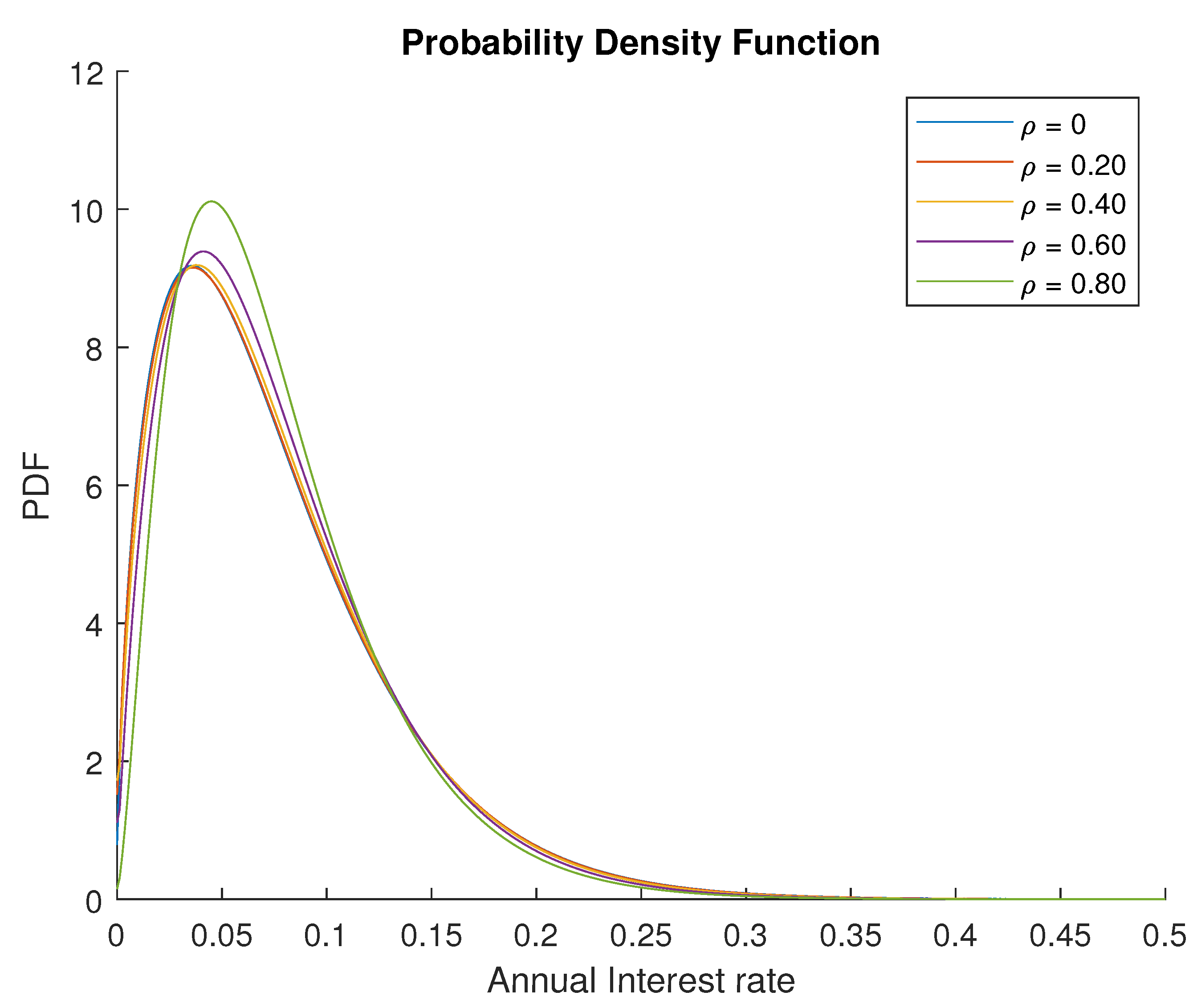
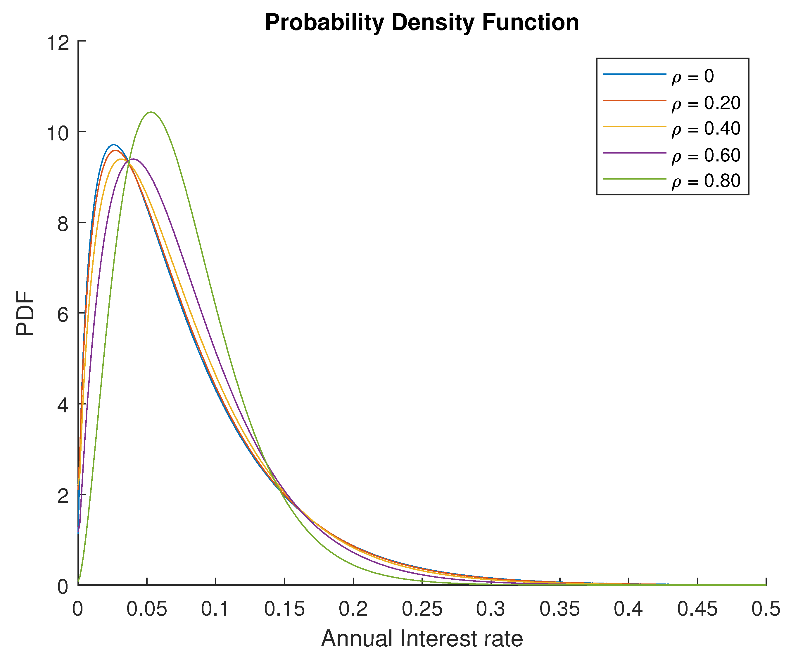
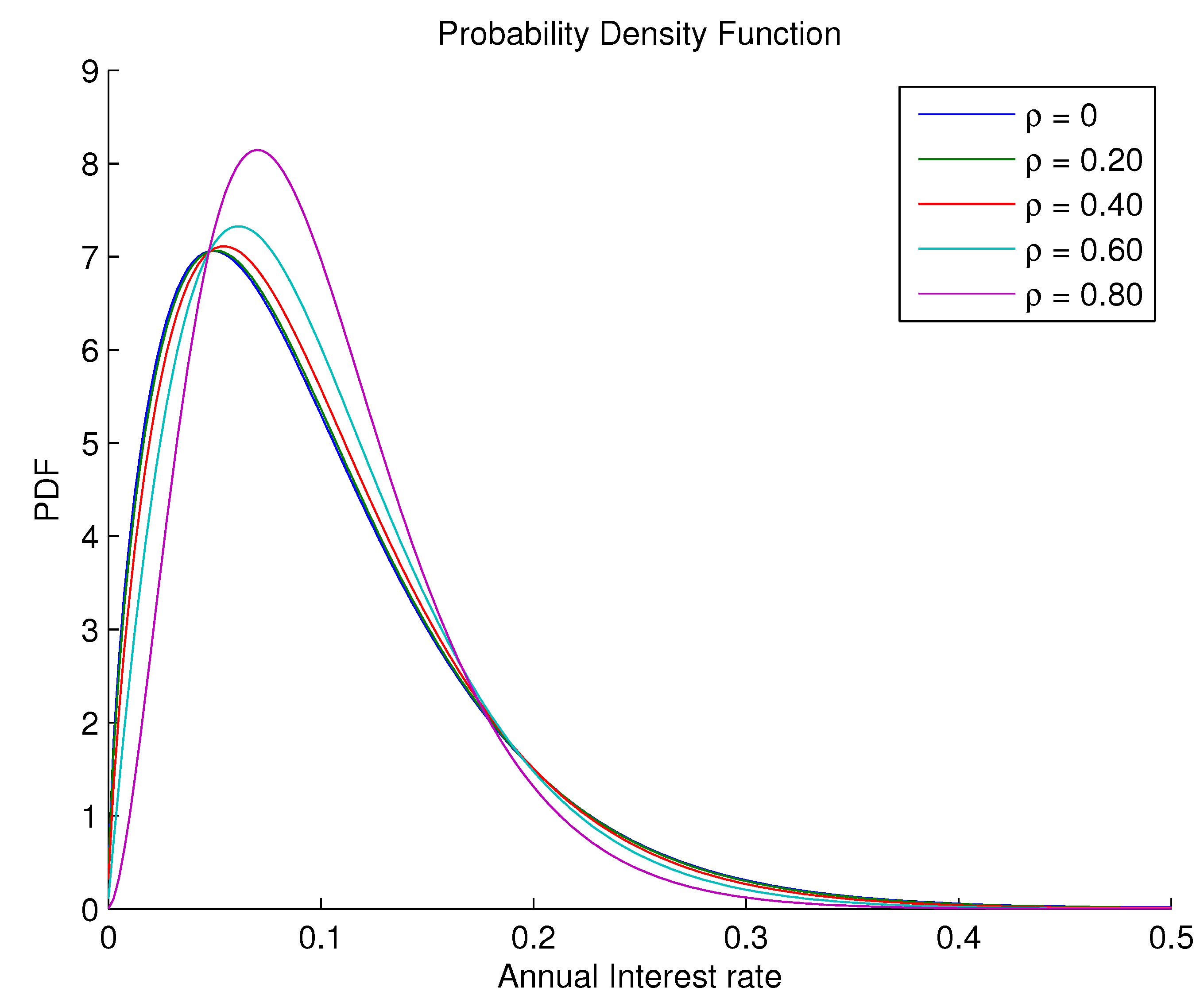
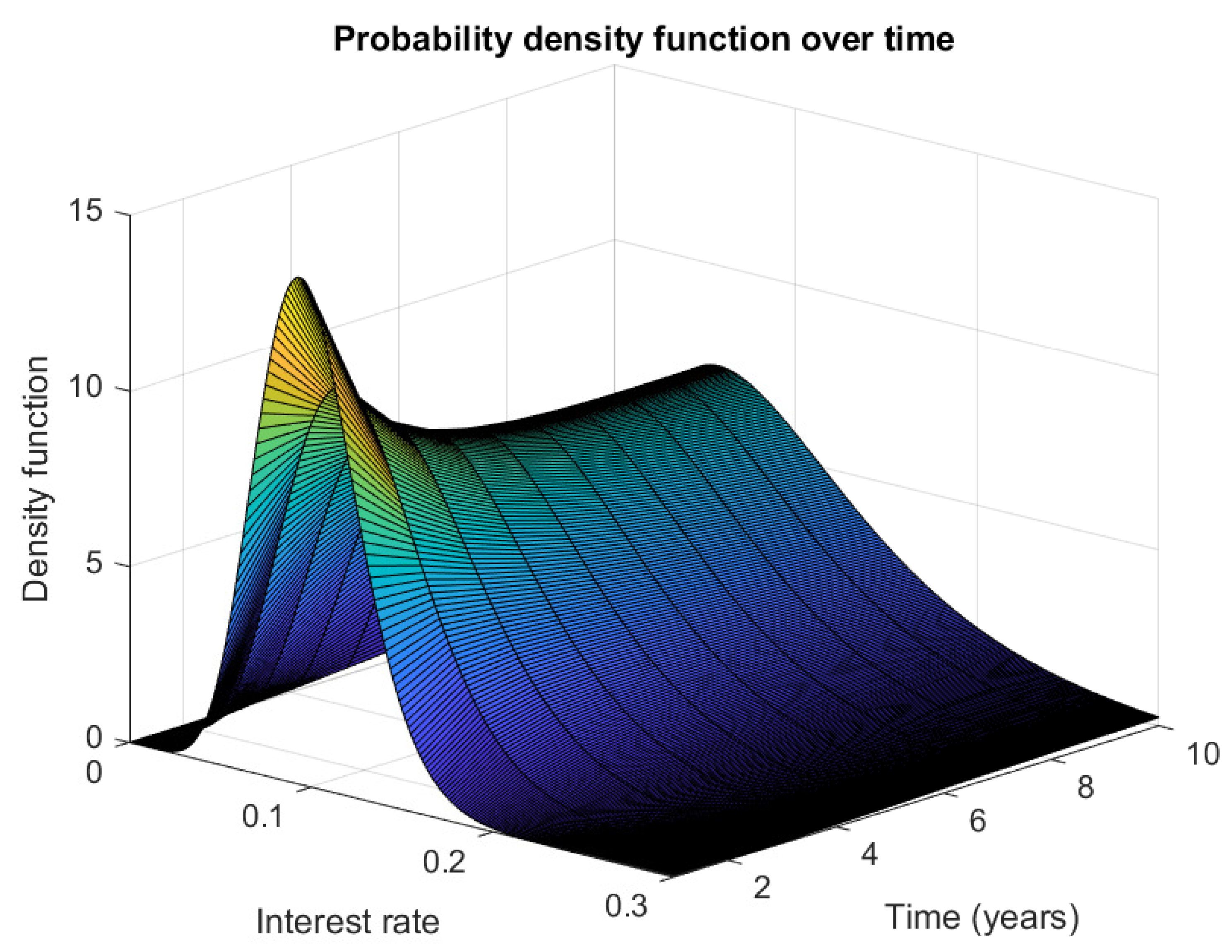
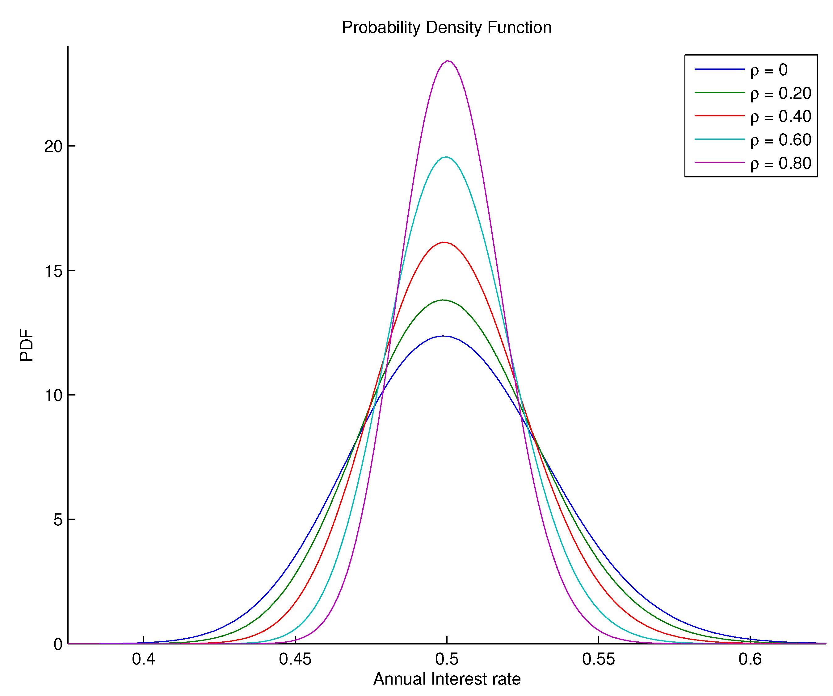
6.3. The Conditional Probability Density Functions of the Short Rate Process

We use the COS method (Fang and Oosterlee 2008) to recover the conditional probability density function of the [ t , T ] -integral of the short rate process R. The approximation of f is given by the following Fourier cosine series
f ( x ) A 0 2 + j = 1 N A j cos j π x a b a , x [ a , b ] ,
for a given N. An analogous result for a discretely distributed random variable can be found in the work of da Silva et al. (2023). If f, with a domain in R , is a probability density function of X, then:
a j 2 b a exp i j π a b a f ^ j π b a A j ,
where f ^ is the characteristic function of X, that is,
f ^ ( u ) = R exp ( i x u ) f ( x ) d x ,
which approximates
a b exp ( i x u ) f ( x ) d x .
We set N = 100 to truncate this series. The parameters A j are given by Equation (36), which in turn is calculated using the characteristic function (12). The same procedure holds to obtain the conditional probability density function of the short-rate process itself at terminal date T, in which case the characteristic function is given by Equation (22).
Setting η 1 = 0 ( η 2 = 0 ), Figure 6 and Figure 7 show the marginal density function for x 1 ( t ) ( x 2 ( t ) ).
Figure 8 shows the ( x 1 ( t ) , x 2 ( t ) ) -conditional probability density functions of R ( T ) versus the correlation parameter ρ . With a high correlation, the thin right tail of the conditional probability density functions of R ( T ) could imply lower probabilities of extreme positive returns and, hence, potentially less attractive derivative pricing under certain market conditions. Conversely, a lower correlation leads to a more positively skewed density, suggesting that the pricing of risk might increase for assets that are more sensitive to idiosyncratic shocks. Such a nuanced understanding of the correlation dynamics between stochastic factors is essential for investors and risk managers alike, as it influences the valuation of bonds and derivatives and the construction of hedging strategies.
It can also be inferred from the figure that the stochastically correlated CIR processes preclude negative values concerning the additive process R, thus preserving the properties of the single- and two-factor uncorrelated square-root diffusion processes (see Figure 9 for the surface of the density over time). Table 2 confirms this statement by presenting the cumulative area under the probability density function for different values of ρ .
Figure 10, in turn, shows the ( x 1 ( t ) , x 2 ( t ) ) -conditional probability density functions of the [ t , T ] -integral of R versus ρ . The lower the correlation parameter, the higher the dispersion. It is worth noting how sensitive the shape of this density function is as we vary the parameter ρ , which suggests that the correlation is a subject matter that cannot be neglected. The probability density function above is used to calculate the price of the IDI option.

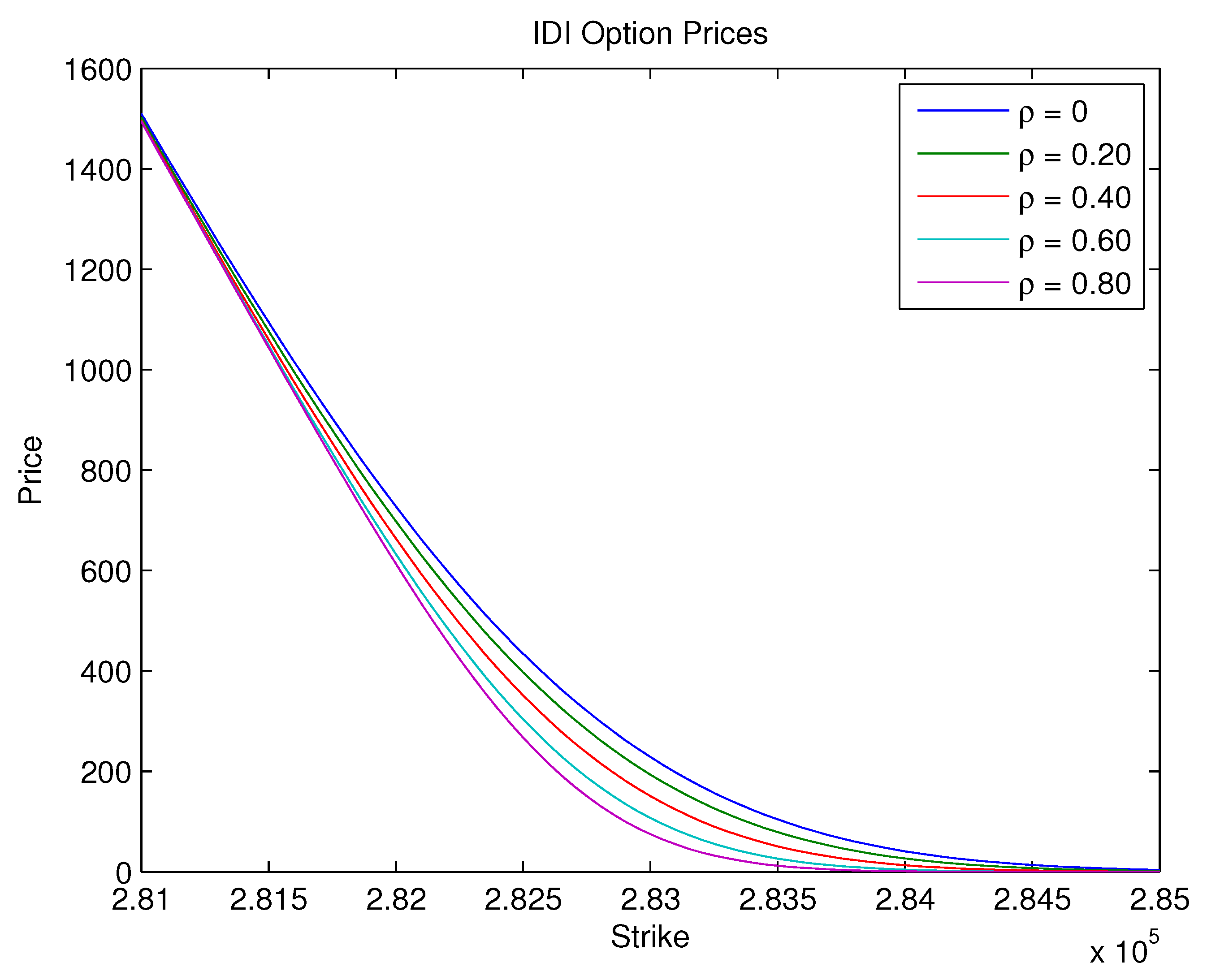
6.4. Pricing the IDI Option

As stated by Fang and Oosterlee (2008), the price of a European option can be approximated as
C ( t , T ) A 0 B 0 2 + j = 1 n A j B j ,
where the A k coefficients are given by (36) and
B j = a b g ( x ) cos j π x a b a d x , for j = 0 , 1 , , n ,
where g ( x ) refers to the payoff of the financial contract.
We assume an interest rate market with an underlying probability space ( Ω , F , Q ) equipped with a filtration F = ( F t ) t [ 0 , T ] , where Q is the risk-neutral measure.
An overnight interest rate r ¯ is the average interbank rate of a one-day period, calculated daily and expressed as the effective rate per annum. According to da Silva et al. (2016), the Interbank Deposit Rate Index (IDI) accumulates discretely, according to
y ( T ) = y ( t ) j = 1 t 1 ( 1 + r ¯ j ) 1 252 ,
where j denotes the end of the day and r ¯ j assigns the corresponding overnight rate.
If we approximate the continuous overnight rate by the instantaneous continuously compounding interest rate, that is, r ( t ) = ln ( 1 + r ¯ ( t ) ) , the index can be represented by the following continuous compounding expression:
y ( T ) = y ( t ) e t T r ( s ) d s .
Given non-negative interest rates, the index is a non-decreasing function of r ( s ) .
A European call option is a contract that gives the owner the right, but not the obligation, to buy a specified amount of underlying security at a specified price and time. The payoff of the IDI call option maturing at T is:
max ( y ( T ) K , 0 ) ,
where K is the strike price. Therefore, the price at time t of this option is
C ( t , T ) = E e t T r ( s ) d s max ( y ( T ) K , 0 ) | r ( t ) = E max y ( t ) K e t T r ( s ) d s , 0 | r ( t ) .
To price the IDI option, we compute the characteristic function of the path-dependent [ t , T ] -integral of the interest rate—namely, x ( t , T ) = t T r ( s ) d s —which in turn gives us the values of A j associated with the model. Therefore, the price of the IDI option can be calculated using the COS method. Equation (44) gives the payoff of the IDI call option so that the coefficients B j are given by
B 0 = ln y ( t ) K b y ( t ) K e x d x = y ( t ) ln y ( t ) K + b 1 + e b K ,
and
B j = ln y ( t ) K b y ( t ) K e x cos π j x a b a d x = { b 2 2 a b + a 2 e b y ( t ) sin π j ln y ( t ) K + π a j b a + ( π a π b ) e b j y ( t ) cos π j ln y ( t ) K + π a j b a + π 2 e b j 2 + b 2 2 a b + a 2 e b sin π j y ( t ) + π b π a j cos π j π 2 j 2 sin π j K } . ( b a ) e b π j π 2 j 2 + b 2 2 a b + a 2 .
The coefficients A j are calculated using (36) according to the characteristic function given by Theorem 1.
Figure 11 depicts the pricing of IDI options over a one-year timeframe with an initial IDI value of y ( t ) = 100.000 and unveils an inverse relationship between the correlation parameter ρ and option prices. In line with the probability density function results, the findings indicate that a decrease in the correlation between the stochastic factors leads to a substantial increase in option prices, with at-the-money options under low-correlation scenarios commanding prices up to fourfold higher than their high-correlation counterparts. This observed phenomenon highlights the crucial impact of the correlation on option valuation, emphasizing its role as a key determinant of market prices. Such revelations have profound implications for interest markets: heightened option prices resulting from lower correlations could signal increased market uncertainty, thereby influencing investment strategies and risk management. Therefore, it is essential to consider the relationship between correlation and pricing, as this may have significant consequences on investment decisions.

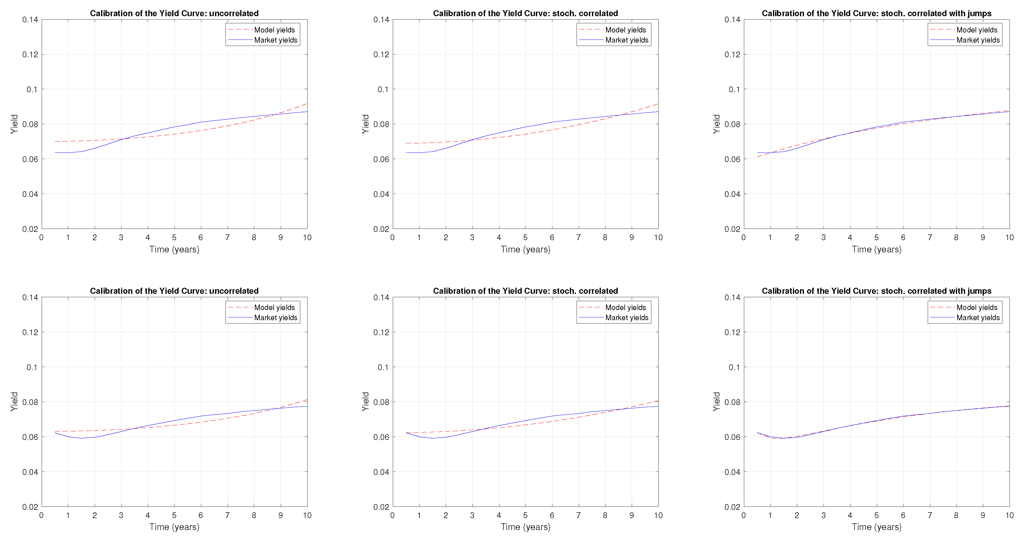
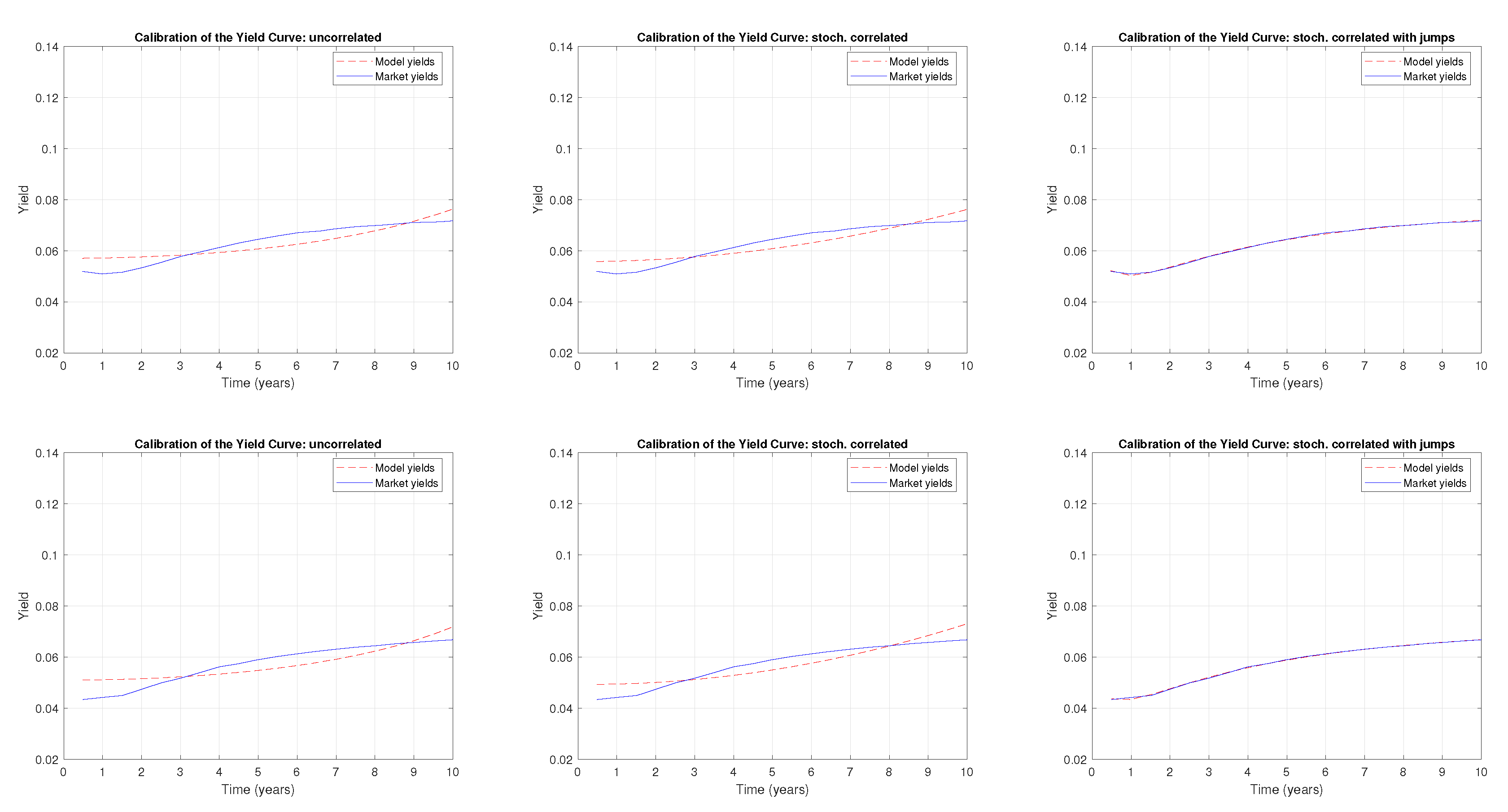
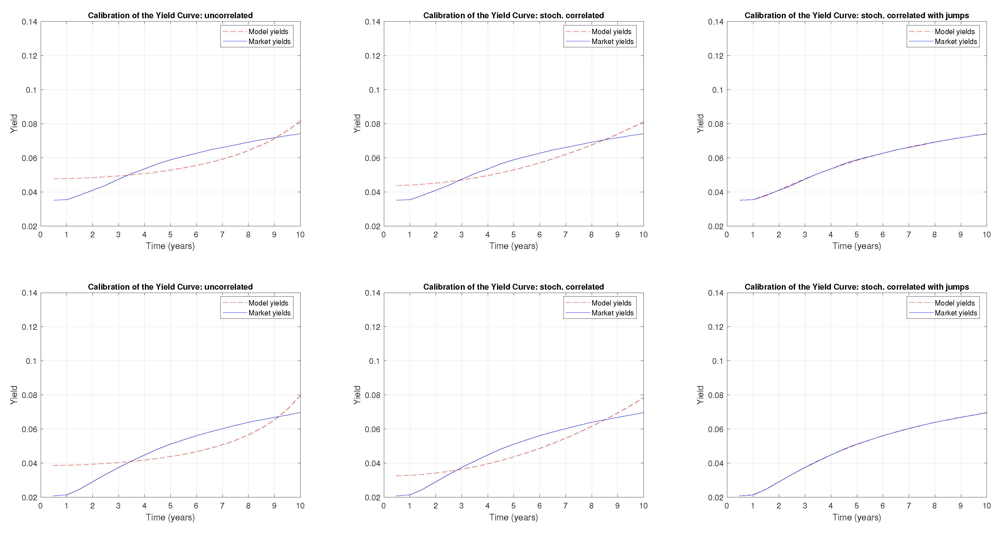
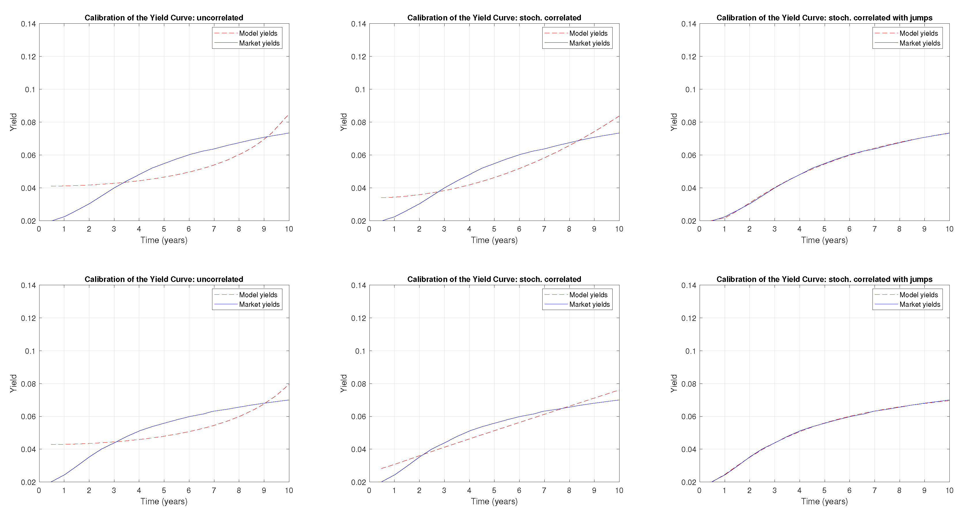
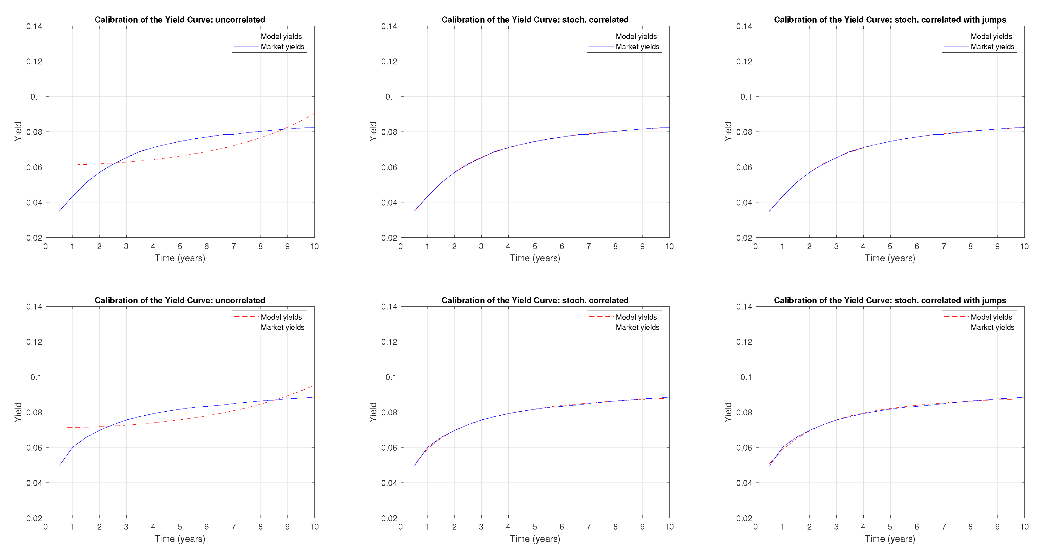
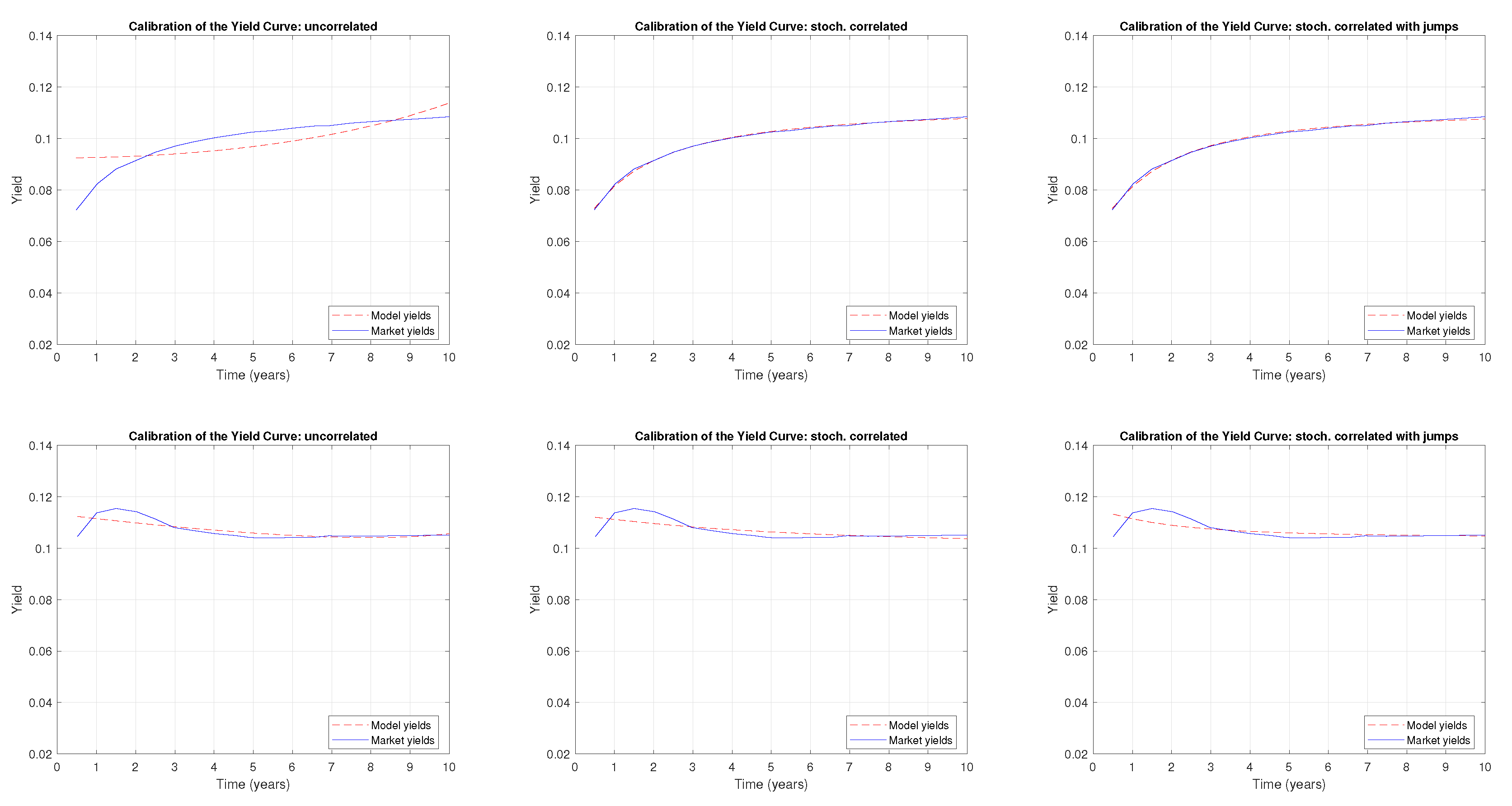
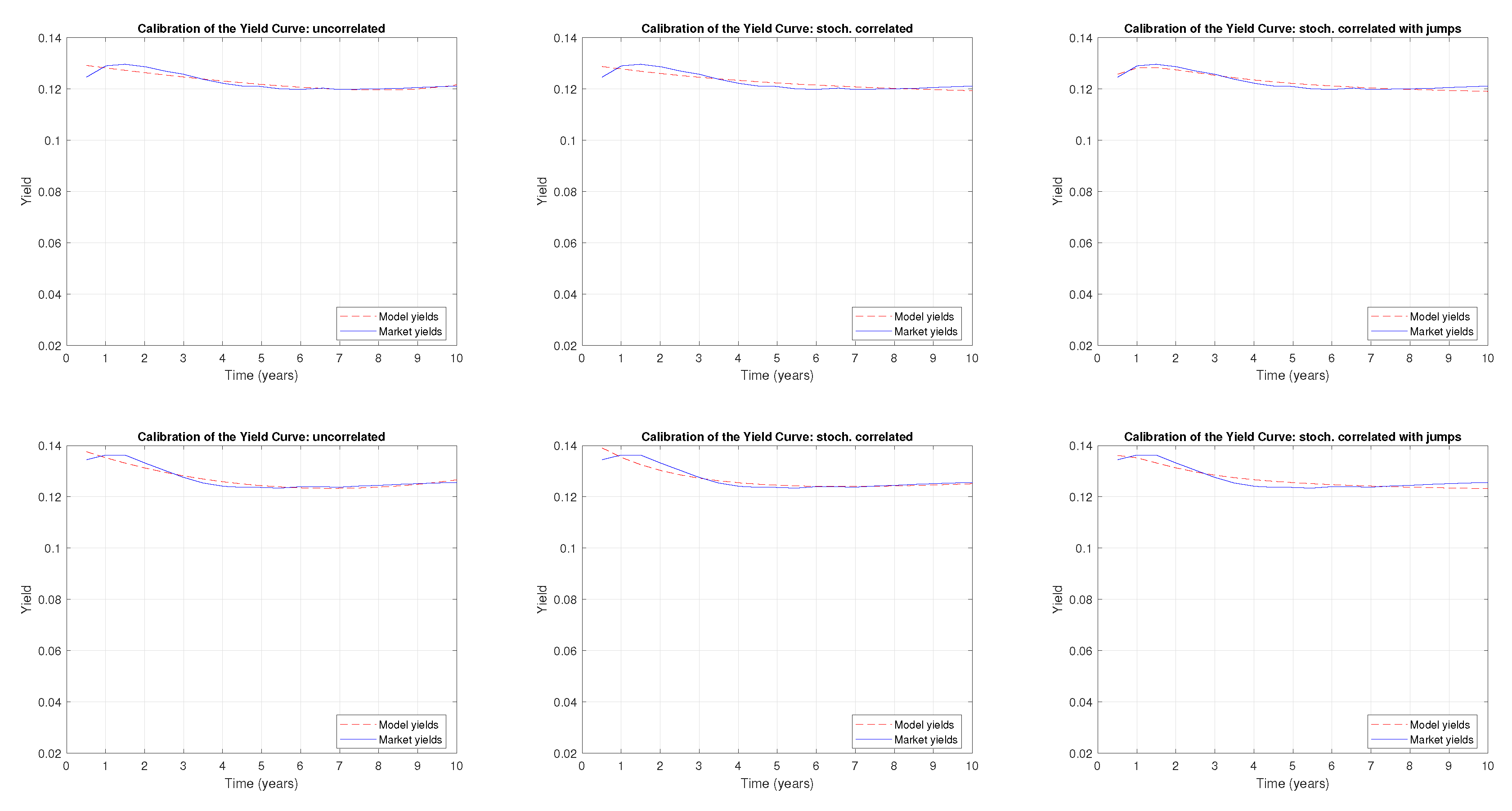
6.5. Term Structure Calibration

We calibrated the term structure of the interest rates over 14 months (from March 2019 to April 2020) with three models. As in the work of da Silva and Baczynski (2024), to test the model in a complex environment, the selected period was marked by abrupt changes in the Brazilian interest rate curve owing to the COVID-19 crisis.
The first model is the uncorrelated two-factor CIR model given by Equations (28) and (29). The estimated parameters are listed in Table 3. The second model is the stochastically correlated two-factor CIR model given by Equations (1), (2), and (4). The corresponding estimated parameters are listed in Table 41.
To show the versatility of the analytical solution developed, we introduce a third model encompassing the stochastically correlated two-factor CIR model enhanced with jumps. The jumps enter to the factor of x 1 such that Equation (1) becomes
d x 1 ( t ) = κ 1 ( θ 1 x 1 ( t ) ) d t + σ 1 x 1 ( t ) d W 1 ( t ) + d J ( t ) .
According to Bouziane (2008), let the jump size J . be exponentially distributed with an expected amplitude η > 0 and constant and positive intensity λ 0 . Therefore, the density function of the jump size is given by
p ( j ; η ) = 1 η e j η j R + .
The term α in Theorem 2 given by Equation (19) is given by the solution of the following differential equation:
α t = κ 1 θ 1 β 1 κ 2 θ 2 β 2 ρ σ 1 σ 2 β 1 β 2 ϵ + λ 0 β 2 η 1 β 2 η .
The estimated parameters of the stochastically correlated two-factor CIR model with exponential jumps are presented in Table 5.
The monthly term structure calibration figures are presented in Appendix A. The left, center, and right figures show the uncorrelated, stochastically correlated, and stochastically correlated jump models, respectively.
The root-mean-squared error between the model and market prices was minimized using the modified sequential quadratic programming method described by (Kienitz and Wetterau 2012, p. 468). The first calibration starts with random initial guess parameter values, and the subsequent guesses come from the calibrated values of the previous month.
It is noteworthy that the stochastically correlated model improves the calibration in comparison with the uncorrelated model for at least 7 of 14 months. Specifically, the error between the calibration and market data is lower in months 7, 8, 9, 10, 11, and 12 of 2019 and in January 2020.
Furthermore, the stochastically correlated jump model shown in the right panels of Appendix A almost matches the yield curves and provides stable correlation and jump parameters over time. The estimated correlation coefficient ρ is approximately 0.55 , the annual frequency of jumps is approximately 10, and the expected jump sizes increase from 50 basis points until the end of 2019 to 800 basis points during the turbulent period. These parameters are coherent with the expected behavior, further validating the model’s effectiveness in capturing market dynamics.

7. Conclusions

Our investigation into the stochastic correlation within a bivariate Cox–Ingersoll–Ross model framework culminated in analytical solutions for conditional moment-generating and characteristic functions. This achievement not only facilitates the derivation of pricing formulas for a spectrum of interest rate derivatives but also provides a robust theoretical underpinning for understanding the complex interdependencies within financial markets. By introducing a variable correlation parameter ( ϵ ), our model adapts to varying degrees of correlation between two factors, offering a flexible tool for capturing a wide array of market behaviors, from tightly integrated markets to those with independent movements.
Theoretically, our model extends the boundaries of stochastic correlation modeling by permitting a dynamic correlation process, which is conspicuously absent in models constrained by a constant correlation assumption. This theoretical advancement translates to a more nuanced and precise modeling of the term structure of interest rates, which is pivotal for both theoretical finance and risk management.
From a practical standpoint, the model’s applicability to the pricing of zero-coupon bonds and Asian options, particularly the IDI option, and the calibration results demonstrate its relevance to market practitioners. Note that obtaining analytical results is not achievable in the case of bivariate CIR models with constant correlation coefficients.
In addition, the simulations herein strongly suggest that the model precludes negative values while preserving the quality of the single- and two-factor uncorrelated CIR process. Calibration showed that enhancing the stochastic correlation model with jumps translates into an almost perfectly calibrated model.
Future research should seek mathematical proof that solidifies the model’s exclusion of negative values for the additive process, as this is a foundational assumption in financial contexts where negative interest rates are precluded. Additionally, it is crucial to identify a specification for stochastic correlation that can accommodate a wider range of correlation values, particularly those approaching the extreme bounds of the correlation spectrum. This would enhance not only the model’s flexibility but also its capacity to mirror the complex dynamics observed in financial markets, where correlations can vary significantly during periods of market stress or tranquility.

Author Contributions

All authors contributed equally to this work. All authors have read and agreed to the published version of the manuscript.

Funding

This research was funded by The National Council for Scientific and Technological Development (CNPq) grant number 140840/2015-0. The APC was funded by the National Laboratory for Scientific Computing (LNCC).

Informed Consent Statement

Not applicable.

Data Availability Statement

The data are available upon request to authors.

Conflicts of Interest

The authors declare no conflicts of interest.

Appendix A. Yield Curve Calibration

Figure A1. A comparison of the term structure calibration with the CIR uncorrelated, CIR stochastically correlated, and CIR stochastically correlated with exponential jump models, respectively, for the following months: March 2019 (upper panels) and April 2019 (lower panels).
Ijfs 12 00031 g0a1
Figure A2. A comparison of the term structure calibration with the CIR uncorrelated, CIR stochastically correlated, and CIR stochastically correlated with exponential jump models, respectively, for the following months: May 2019 (upper panels) and June 2019 (lower panels).
Ijfs 12 00031 g0a2
Figure A3. A comparison of the term structure calibration with the CIR uncorrelated, CIR stochastically correlated, and CIR stochastically correlated with exponential jump models, respectively, for the following months: July 2019 (upper panels) and August 2019 (lower panels).
Ijfs 12 00031 g0a3
Figure A4. A comparison of the term structure calibration with the CIR uncorrelated, CIR stochastically correlated, and CIR stochastically correlated with exponential jump models, respectively, for the following months: September 2019 (upper panels) and October 2019 (lower panels).
Ijfs 12 00031 g0a4
Figure A5. A comparison of the term structure calibration with the CIR uncorrelated, CIR stochastically correlated, and CIR stochastically correlated with exponential jump models, respectively, for the following months: November 2019 (upper panels) and December 2019 (lower panels).
Ijfs 12 00031 g0a5
Figure A6. A comparison of the term structure calibration with the CIR uncorrelated, CIR stochastically correlated, and CIR stochastically correlated with exponential jump models, respectively, for the following months: January 2020 (upper panels) and February 2020 (lower panels).
Ijfs 12 00031 g0a6
Figure A7. A comparison of the term structure calibration with the CIR uncorrelated, CIR stochastically correlated, and CIR stochastically correlated with exponential jump models, respectively, for the following months: March 2020 (upper panels) and April 2020 (lower panels).
Ijfs 12 00031 g0a7

Note

1
We truncated the values to three decimal places.

References

  1. Almeida, Caio, and José V. M. Vicente. 2009. Are interest rate options important for the assessment of interest rate risk? Journal of Banking and Finance 33: 1376–1387. [Google Scholar] [CrossRef]
  2. Bertini, Lorenzo, and Luca Passalacqua. 2008. Modelling interest rates by correlated multi-factor cir-like processes. arXiv arXiv:0807.3898. [Google Scholar] [CrossRef]
  3. Bouziane, Markus. 2008. Pricing Interest-Rate Derivatives: A Fourier-Transform Based Approach. Berlin: Springer. [Google Scholar]
  4. Brigo, Damiano, and Fabio Mercurio. 2006. Interest Rate Models—Theory and Practice. Springer Finance. Berlin: Springer. [Google Scholar]
  5. Cox, John C., Jonathan E. Ingersoll, Jr., and Stephen A. Ross. 1986. A theory of the term structure of interest rates. Econometrica 53: 385–407. [Google Scholar] [CrossRef]
  6. da Silva, Allan Jonathan, and Jack Baczynski. 2024. Discretely distributed scheduled jumps and interest rate derivatives: Pricing in the context of central bank actions. Economies 12: 73. [Google Scholar] [CrossRef]
  7. da Silva, Allan Jonathan, Jack Baczynski, and J. F. Silva Bragança. 2019. Path-dependent interest rate option pricing with jumps and stochastic intensities. In Computational Science—ICCS 2019. Lecture Notes in Computer Science. Cham: Springer, vol. 11540, pp. 710–16. [Google Scholar] [CrossRef]
  8. da Silva, Allan Jonathan, Jack Baczynski, and José Valentim Machado Vicente. 2016. A new finite method for pricing and hedging fixed income derivatives: Comparative analysis and the case of an Asian option. Journal of Computational and Applied Mathematics 297: 98–116. [Google Scholar] [CrossRef]
  9. da Silva, Allan Jonathan, Jack Baczynski, and José Valentim Machado Vicente. 2023. Recovering probability functions with fourier series. Pesquisa Operacional 43: e267882. [Google Scholar] [CrossRef]
  10. Duffie, Darrell. 2001. Dynamic Asset Pricing Theory. Princeton Series in Finance. Princeton: Princeton University Press. [Google Scholar]
  11. Duffie, Darrel, and Kenneth J. Singleton. 2003. Credit Risk: Pricing, Measurement, and Management. Princeton: Princeton University Press. [Google Scholar]
  12. Fang, Fang, and Cornelis W. Oosterlee. 2008. A novel pricing method for European options based on Fourier-cosine series expansions. SIAM Journal on Scientific Computing 31: 826–48. [Google Scholar] [CrossRef]
  13. Fisher, Irving. 1930. The Theory of Interest. New York: Macmillan. [Google Scholar]
  14. Glasserman, Paul. 2004. Monte Carlo Methods in Financial Engineering. Applications of Mathematics: Stochastic Modelling and Applied Probability. New York: Springer. [Google Scholar]
  15. Harrison, Michael, and Stanley Pliska. 1981. Martingales and stochastic integrals in the theory of continuous trading. Stochastic Processes and their Applications 11: 215–60. [Google Scholar] [CrossRef]
  16. Jamshidian, Farshid, and Yu Zhu. 1997. Scenario simulation: Theory and methodology. Finance and Stochastics I: 43–67. [Google Scholar]
  17. Kienitz, Joerg, and Daniel Wetterau. 2012. Financial Modelling: Theory, Implementation and Practice with MATLAB Source. The Wiley Finance Series; Hoboken: Wiley. [Google Scholar]
  18. Kim, Jongwook, and Junghyo Jo. 2014. Correlated stochastic processes in financial markets. Physica A 406: 230–35. [Google Scholar] [CrossRef]
  19. Kim, Young Shin, Hyangju Kim, Jaehyung Choi, and Frank J. Fabozzi. 2023. Multi-asset option pricing using normal tempered stable processes with stochastic correlation. The Journal of Derivatives 30: 42–64. [Google Scholar] [CrossRef]
  20. Leippold, Markus, and Fabio Trojani. 2010. Matrix Affine Jump Diffusions for Multivariate Risk Modeling. Available online: https://ssrn.com/abstract=1274482 (accessed on 18 March 2024).
  21. Luo, Cuicui, and Luis Seco. 2017. Stochastic correlation in risk analytics: A financial perspective. IEEE Systems Journal 11: 1479–85. [Google Scholar] [CrossRef]
  22. Márkus, László, and Ashish Kumar. 2019. Comparison of stochastic correlation models. Journal of Mathematical Sciences 237: 810–18. [Google Scholar] [CrossRef]
  23. Márkus, László, and Ashish Kumar. 2021. Modelling joint behaviour of asset prices using stochastic correlation. Methodology and Computing in Applied Probability 23: 341–54. [Google Scholar] [CrossRef]
  24. Musiela, Marek, and Marek Rutkowski. 1998. Martingale Methods in Financial Modelling. Berlin and Germany: Springer. [Google Scholar]
  25. Oksendal, Bernt. 2007. Stochastic Differential Equations, 6th ed. New York: Springer. [Google Scholar]
  26. Protter, Philip E. 2005. Stochastic Integration and Differential Equations. Berlin and Heidelberg: Springer. [Google Scholar] [CrossRef]
  27. Reid, William Thomas. 1972. Riccati Differential Equations. Mathematics in Science and Engineering: A Series of Monographs and Textbooks. Cambridge, MA: Academic Press. [Google Scholar]
  28. Ross, Sheldon M. 2007. Introduction to Probability Models. Amsterdam: Elsevier Science. [Google Scholar]
  29. Stehlíková, Beáta. 2020. On the bond pricing partial differential equation in a convergence model of interest rates with stochastic correlation. Mathematica Slovaca 70: 995–1002. [Google Scholar] [CrossRef]
  30. Teng, Long, Matthias Ehrhardt, and Michael Günther. 2017. Modelling and Calibration of Stochastic Correlation in Finance. In Novel Methods in Computational Finance. Cham: Springer. [Google Scholar] [CrossRef]
  31. Vasicek, Oldrich. 1977. An equilibrium characterization of the term structure. Journal of Financial Economics 5: 177–88. [Google Scholar] [CrossRef]
Figure 1. Stochastically correlated paths generated randomly according to the model (1)–(4) with parameters κ 1 = 0.15 , κ 2 = 0.15 , θ 1 = 0.05 , θ 2 = 0.05 , σ 1 = 0.015 , σ 2 = 0.025 , ρ = 0.5 , T t = 1 year, and initial condition x 1 ( 0 ) = 0.05 and x 2 ( 0 ) = 0.05 .
Ijfs 12 00031 g001
Figure 2. The instantaneous stochastic correlation coefficient path. The random sample of ϱ ( t , ω ) evolves according to the model (1)–(4) with parameters κ 1 = 0.15 , κ 2 = 0.15 , θ 1 = 0.05 , θ 2 = 0.05 , σ 1 = 0.015 , σ 2 = 0.025 , ρ = 0.5 , T t = 1 year, and initial condition x 1 ( 0 ) = 0.05 and x 2 ( 0 ) = 0.05 .
Ijfs 12 00031 g002
Figure 3. The stochastic correlation mean for each ρ . The means of ϱ ( t , ω ) for varying ρ were calculated from n = 1000 paths where the model evolves according to (1)–(4) with parameters κ 1 = 0.15 , κ 2 = 0.15 , θ 1 = 0.05 , θ 2 = 0.05 , σ 1 = 0.015 , σ 2 = 0.025 , T t = 1 year, and initial condition x 1 ( 0 ) = 0.05 and x 2 ( 0 ) = 0.05 .
Ijfs 12 00031 g003
Figure 4. The stochastic correlation mean for each ρ and ϵ calculated from n = 1000 paths where the model evolves according to (1)–(4) with parameters κ 1 = 0.15 , κ 2 = 0.15 , θ 1 = 0.05 , θ 2 = 0.05 , σ 1 = 0.015 , σ 2 = 0.025 , T t = 1 year, and initial condition x 1 ( 0 ) = 0.05 and x 2 ( 0 ) = 0.05 .
Ijfs 12 00031 g004
Figure 5. The stochastic correlation standard deviation for each ρ and ϵ calculated from n = 1000 paths where the model evolves according to (1)–(4) with parameters κ 1 = 0.15 , κ 2 = 0.15 , θ 1 = 0.05 , θ 2 = 0.05 , σ 1 = 0.015 , σ 2 = 0.025 , T t = 1 year, and initial condition x 1 ( 0 ) = 0.05 and x 2 ( 0 ) = 0.05 .
Ijfs 12 00031 g005
Figure 6. The probability density functions of x 1 ( t ) using the Fourier cosine series given by (35), where the characteristic function is given by the result of Theorem 2.
Ijfs 12 00031 g006
Figure 7. The probability density functions of x 2 ( t ) using the Fourier cosine series given by (35), where the characteristic function is given by the result of Theorem 2.
Ijfs 12 00031 g007
Figure 8. The ρ -parameterized density functions of R ( T ) using the Fourier cosine series given by (35), where the characteristic function is given by the result of Theorem 2.
Ijfs 12 00031 g008
Figure 9. The evolution of the density function of R ( T ) over time using the Fourier cosine series given by Equation (35), where the characteristic function is given by the result of Theorem 2.
Ijfs 12 00031 g009
Figure 10. The ρ -parameterized density functions of t T R ( s ) d s using the Fourier cosine series given by Equation (35), where the characteristic function is given by the result of Theorem 1.
Ijfs 12 00031 g010
Figure 11. IDI option prices calculated according to the formula given by (39). The characteristic function is given by the formula developed in Theorem 2 and the coefficients B j are given by (46).
Ijfs 12 00031 g011
Table 1. Parameter values. Source: Almeida and Vicente (2009).
Parameter κ 1 κ 2 κ 3 θ 1 θ 2 θ 3 σ 1 σ 2 σ 3
Value11.18190.00032.03110.02914.74850.0430.15070.05180.1228
Table 2. Numerical integral value of probability density function.
ρ 00.20.40.60.80.910.930.950.970.99
I1.00021.00051.00051.00031.00001.00001.00001.00001.00001.0000
Table 3. Parameter values for the uncorrelated model.
σ 1 σ 2 θ 1 θ 2 κ 1 κ 2 x 1 x 2
0.1170.1170.0180.0130.0000.0000.0170.053
0.1260.1130.0000.0010.0040.0000.0060.057
0.1200.1200.0000.0010.0000.0000.0100.047
0.1280.1280.0150.0040.0000.0000.0230.028
0.1520.1520.0150.0040.0000.0000.0230.024
0.1670.1670.0070.0000.0000.0000.0180.021
0.1670.1670.0070.0000.0000.0000.0190.022
0.1590.1590.0060.0000.0000.0000.0200.022
0.1350.1350.0030.0000.0000.0000.0300.031
0.1200.1210.0000.0060.0000.0000.0360.035
0.1040.1040.0120.0060.0000.0000.0450.048
0.0010.1440.1190.0560.0170.0000.0970.017
0.0000.1570.1740.0530.0140.0000.1170.013
0.0040.0760.0440.0340.2420.0000.0020.138
Table 4. Parameter values for the stochastic correlation model.
σ 1 σ 2 θ 1 θ 2 κ 1 κ 2 ρ ϵ x 1 x 2
0.0740.1530.0000.0000.0000.0001.0000.0500.0310.038
0.0550.1610.0030.0210.0000.0000.9990.0500.0620.000
0.0180.6720.0010.0960.0000.0001.0000.0500.0480.008
0.0250.6690.0000.0920.0060.0001.0000.0440.0420.008
0.0310.7020.0110.0920.0000.0001.0000.0490.0420.002
0.0480.7000.0070.0870.0000.0001.0000.0390.0310.001
0.0221.4720.0000.0870.0000.0001.0000.0460.0210.013
0.1883.2350.0000.0032.2830.0001.0000.0370.0000.027
2.6572.6790.0030.0003.7971.5701.0000.0460.0000.035
3.00619.9990.0000.00015.0263.8010.9910.0500.0020.039
4.01419.9990.0000.00014.8434.0870.9900.0490.0000.069
0.54719.6020.0000.00015.2730.3521.0000.0500.0000.113
0.60019.6010.0000.00015.2710.3351.0000.0500.0000.130
0.59219.6010.0020.00815.2710.3671.0000.0450.0010.146
Table 5. Parameter values for the stochastic correlation model with jumps.
σ 1 σ 2 θ 1 θ 2 κ 1 κ 2 ρ ϵ x 1 x 2 λ 0 η
0.0520.0030.1800.0070.1830.1440.0000.0250.0590.0009.9870.006
0.2170.5580.0010.0300.4543.1440.5180.0500.0730.00210.0880.005
0.1500.5580.0150.0110.5553.1460.5210.0500.0380.02510.0870.006
0.1640.5590.0160.0170.5333.1430.5200.0480.0420.00910.0870.006
0.2120.5580.0000.0250.4273.1410.5190.0430.0380.00510.0880.004
0.1910.5590.0000.0300.4323.1400.5200.0460.0230.00710.0890.005
0.1280.5610.0000.0280.4243.1380.5240.0500.0200.00810.1010.005
0.0000.5760.0010.0130.5103.2590.6070.0490.0120.00810.3850.005
0.0350.5740.0000.0090.9093.2680.6100.0500.0230.00310.4130.009
0.0310.5740.0000.0000.9603.2680.6100.0500.0400.00010.4100.009
0.0230.5730.0140.0001.0723.2690.6100.0500.0610.00010.3990.013
0.0210.5730.0800.0001.1203.2690.6100.0490.1160.00010.3940.020
0.0000.5790.6350.0000.9313.2640.6150.0500.1170.00010.1040.075
0.0000.5940.5180.0001.3233.1610.6070.0320.1320.00010.2210.088
Disclaimer/Publisher’s Note: The statements, opinions and data contained in all publications are solely those of the individual author(s) and contributor(s) and not of MDPI and/or the editor(s). MDPI and/or the editor(s) disclaim responsibility for any injury to people or property resulting from any ideas, methods, instructions or products referred to in the content.

