Predicting Healthcare Mutual Fund Performance Using Deep Learning and Linear Regression

Abstract

Following the COVID-19 pandemic, the healthcare sector has emerged as a resilient and profitable domain amidst market fluctuations. Consequently, investing in healthcare securities, particularly through mutual funds, has gained traction. Existing research on predicting future prices of healthcare securities has been predominantly reliant on historical trading data, limiting predictive accuracy and scope. This study aims to overcome these constraints by integrating a diverse set of twelve external factors spanning economic, industrial, and company-specific domains to enhance predictive models. Employing Long Short-Term Memory (LSTM) and Multiple Linear Regression (MLR) techniques, the study evaluates the effectiveness of this multifaceted approach. Results indicate that incorporating various influencing factors beyond historical data significantly improves price prediction accuracy. Moreover, the utilization of LSTM alongside this comprehensive dataset yields comparable predictive outcomes to those obtained solely from historical data. Thus, this study highlights the potential of leveraging diverse external factors for more robust forecasting of mutual fund prices within the healthcare sector.

1. Introduction

The capital market is a crucial source for mobilizing savings and providing long-term credit in Thailand (Wanaset 2018). It plays a significant role in the country’s economic development. The capital market provides a platform for buying and selling securities such as stocks and bonds, where mutual funds actively participate by pooling funds from investors to invest in these securities. A mutual fund serves as an investment vehicle that aggregates funds from numerous investors, directing them towards a diversified portfolio encompassing various asset classes such as stocks, bonds, and other securities. The inherent advantages of mutual fund investment include risk mitigation through diversification, expert management by seasoned fund managers, and the convenience of daily liquidity, enabling investors to buy or sell shares on a daily basis. Opting for mutual funds proves to be an appealing choice for individuals looking to capitalize on diversified returns while benefiting from the expertise of professional fund management.

In the midst of the market volatility precipitated by the onset of the global COVID-19 pandemic in early 2020, central banks and ministries of finance across diverse nations initiated a series of policy interventions known as Quantitative Easing (QE). These interventions encompassed measures such as interest rate reductions, infusion of liquidity into the financial system, and the implementation of stimulus packages spanning various sectors throughout the period spanning 2020 to 2021. The primary objective of these policies was to mitigate the adverse economic repercussions stemming from the COVID-19 crisis. However, the implementation of these measures inadvertently triggered an uptick in inflation rates across several nations in 2022, thereby prompting a swift and robust response from central banking authorities, including the U.S. Federal Reserve (Fed) and the European Central Bank (ECB). This response entailed a decisive tightening of monetary policy, characterized by aggressive interest rate hikes aimed at curbing inflationary pressures. Consequently, global equity markets experienced notable corrections, with returns on diverse asset classes registering downward adjustments commensurate with the prevailing market dynamics.

While 2022 witnessed pronounced market volatility, it is essential to note that not all sectors encountered uniform challenges. Notably, the healthcare sector demonstrated resilience and commendable performance amidst market fluctuations, attributable to several key factors. Firstly, healthcare stocks exhibited robust financial performance in recent periods, showcasing their ability to weather economic downturns and navigate high market volatility (Dillender et al. 2021). Secondly, external dynamics such as the COVID-19 pandemic, the aging global population, and advancements in medical technology significantly contributed to the sector’s substantial growth. Thirdly, the healthcare sector maintains an appealing valuation, characterized by comparatively lower profit estimates in relation to other sectors, thus eliciting interest in exploring investment opportunities within healthcare securities. Given the favorable prospects for the healthcare industry, concerted efforts are underway to leverage and capitalize on the profit potential inherent in healthcare securities. One notable strategy involves the application of Machine Learning Models for forecasting future returns, thereby offering valuable insights to guide investment decisions within the healthcare sector.

Machine Learning (ML) has been increasingly integrated into investment strategies, enabling computer systems to process, predict, and make decisions independently through learning from input datasets (Alzubi et al. 2018; Janiesch et al. 2021). This approach empowers computers to autonomously handle and solve various problems by learning from the data fed into them. ML operates on principles similar to human learning, requiring the assimilation of experiences. In ML, the process involves feeding data and instructions to the computer for learning. To enhance outcomes, continuous input of new data is necessary, fostering consistent learning and model refinement. ML is categorized into three types: Supervised Learning, Unsupervised Learning, and Reinforcement Learning. Among these, Multiple Linear Regression (MLR) is a fundamental algorithm in supervised learning (Slinker and Glantz 1988). MLR requires data input for the model to learn, employing statistical calculations to produce numerical results. MLR finds applications in various fields, including the environment (Heshmaty and Kandel 1985), agriculture (Kittichotsatsawat et al. 2022), and finance (Alnabulsi et al. 2023), showcasing its versatility.

One of the most popular and widely discussed branches is Deep Learning (Kumar and Manash 2019). It is a mathematical model that mimics the workings of the neural networks in the human brain by combining multiple layers of neural networks into a highly complex architecture (Sarker 2021). This complexity makes it an efficient and highly accurate mathematical model. Deep Learning involves learning from sample data, and the acquired knowledge is then used for tasks such as pattern recognition, data categorization, or data prediction (Kumar and Manash 2019). Later developments in Deep Learning led to the creation of a mathematical model known as Long Short-Term Memory (LSTM).

LSTM, a recurrent neural network model tailored for time-series data analysis (Hochreiter and Schmidhuber 1997), demonstrates proficiency in handling vast datasets and decision-making, surpassing conventional artificial neural networks (Hochreiter and Schmidhuber 1997; Van Houdt et al. 2020). Modeled after the memory patterns of the human brain, LSTM possesses a constrained memory capacity, akin to the brain’s process of discerning the significance of new events for acceptance or rejection (Hochreiter and Schmidhuber 1997). This distinctive architecture empowers LSTM to excel in capturing patterns from prolonged sequences (Bolboacă and Haller 2023; Hochreiter and Schmidhuber 1997; Van Houdt et al. 2020), rendering it well suited for analyzing time-series data, including historical stock prices (Ouyang et al. 2020; Gülmez 2023).

As mentioned earlier, investing in mutual funds involves risks stemming from the price volatility influenced by various factors (Banegas et al. 2022; Li 2020; Qureshi et al. 2017). In addition to the managerial capabilities in selecting investments in different fund units, external factors may also impact the fund’s price volatility, particularly concerning economic issues (Kang et al. 2022). This study has therefore categorized the influencing factors into two groups: internal factors, involving the investment choices in various assets directly affecting the fund’s price, and external factors, encompassing economic indicators reflecting market conditions and the country’s economic state over time (Panigrahi et al. 2019). Both groups of factors are considered crucial and are diligently incorporated into the dataset to create a model capable of accurate and efficient predictions.

This study proposes the use of the MLR and LSTM model to forecast the trends in the prices of mutual funds in the healthcare sector in Thailand during the post-COVID-19 period. The approach involves utilizing external factors, which are economic indicators expected to influence the securities prices in the medical business sector based on previous studies. Additionally, internal factors such as past asset prices selected by the fund for investment are incorporated. Our study presents a paradigm shift in stock market prediction, going beyond the confines of historical trading data. The results illuminate the efficacy of incorporating various factors that influence the healthcare sector for accurate future price predictions. Notably, our exploration reveals that the application of Long Short-Term Memory (LSTM) models to this diverse set of data produces results on par with traditional methods reliant solely on historical data for forecasting. This breakthrough underscores the potential for a more robust and comprehensive approach to forecasting stock prices.

The above passage outlines the structure of the research study. It begins by highlighting the origin and significance of the identified gaps in previous literature and the introduction of machine learning tools. Following this, the study will proceed with a review of previous research, identification of gaps in the existing literature, and a comparative analysis of research outcomes similar to the current study. Subsequently, the methodology of the study will be comprehensively presented. The subsequent section will focus on a detailed discussion of the findings, including an exploration of the study’s limitations. Finally, the study will be concluded by summarizing the results and suggesting potential directions for future research.

2. Literature Review

Brogaard and Zareei (2023) utilize machine learning algorithms to explore the profitability of technical trading rules based on historical stock prices. Their study confirms investors’ ability to discover profitable rules through machine learning methods. Comparisons with other algorithms highlight evolutionary genetic algorithms’ advantage in incorporating erroneous predictions, resulting in enhanced profitability. Evaluation across various periods consistently shows the selection of trading rules that perform well out of sample, maximizing abnormal returns. Additional tests on diverse datasets ensure the robustness of the findings. This research demonstrates the potential of utilizing machine learning in finance, particularly in employing complex and efficient models for computational tasks. The findings suggest that the methodologies and insights derived from this study can be extrapolated to other models, particularly those with high computational complexity and efficiency, for application in finance-related endeavors.

The utilization of machine learning, particularly in the form of deep learning models, has witnessed a notable surge within the realm of finance. Gu et al. (2020) elucidate that machine learning methodologies substantially augment empirical asset pricing frameworks, surpassing conventional regression-based methodologies. Their study delineates decision trees and neural networks as preeminent performers, adept at capturing intricate nonlinear interactions among predictors. A consensus emerges regarding the prominence of predictive signals such as momentum, liquidity, and volatility. These methodologies proffer discerning insights for investors, potentially amplifying the efficacy of conventional strategies twofold, with a pronounced proficiency in forecasting returns for sizable, more liquid equities and portfolios. This underscores the burgeoning influence of machine learning within the fintech domain.

In a parallel vein, Zhou et al. (2023) employ deep neural network (DNN) models to predict the US equity premium, comparing their efficacy against ordinary least squares (OLS) and historical average (HA) models. The investigation reveals that DNN models consistently outshine OLS and HA counterparts across in-sample and out-of-sample assessments, alongside asset allocation simulations. Moreover, the integration of 14 supplementary variables sourced from finance literature bolsters the predictive accuracy of DNN models. Notably, the paper introduces a nonlinear machine learning paradigm for forecasting equity premiums, marking a departure from conventional econometric frameworks. Additionally, the study delineates the foundational equations underpinning the employed DNN models.

The points highlighted in the study review by Sonkavde et al. (2023) align with the recognition of deep learning models’ prominence in the financial sector, particularly in stock price prediction and classification. The review underscores that deep learning models, with their capability to capture intricate patterns, handle extensive datasets, and engage in feature learning and representation, have gained popularity in forecasting and trend prediction for stock prices. Similarly, the findings from Shah et al. (2022), who discussed the limitations and accuracy of various models, including deep learning, support the notion that deep learning algorithms, such as LSTM, Convolutional Neural Networks (CNN), and their hybrid models, significantly impact stock prediction and portfolio management.

During the recent COVID-19 situation, there have been research efforts employing deep learning models to study forecasting trends. Ersin and Bildirici (2023) proposed the GARCH-MIDAS-LSTM model, which integrates LSTM deep neural networks with the GARCH-MIDAS model to predict stock market volatility. This research utilized data from the Borsa Istanbul stock market, specifically during the COVID-19 shutdown and economic reopening period in Turkey. An important aspect of this research is the incorporation of monthly explanatory variables, encompassing economic leading indicators such as the Composite Leading Index (CLI), the country-specific Geopolitical Risk Index (GPR) for Türkiye, and the cycle and trend industrial production indices (IPIC and IPIT). The findings indicate that stock market volatility is most effectively modeled with geopolitical risk, followed by industrial production, while the impact of future economic expectations is relatively lower. This demonstrates the capability of utilizing deep learning models during the COVID-19 situation and additionally highlights the integration of economic indicators in model development.

Similarly to Chimmula and Zhang (2020), who developed a Deep Learning forecasting model for COVID-19 in Canada utilizing LSTM networks for real-time predictions, this study demonstrates superior performance compared to other models. The model provides valuable insights into transmission rates across countries and serves as an alert system for frontline staff, aiding in crisis preparations. Key findings of the study include identifying a linear transmission trend in Canada, predicting an expected end within three months, and highlighting the model’s effectiveness in guiding health authorities. The research underscores the impact of early social distancing measures and emphasizes the potential role of technology and international collaboration. In summary, the developed model presents a valuable tool for crisis management and prevention. However, all previous research works have not conducted in-depth studies in the healthcare sector.

In the domain of predicting healthcare stock prices, research employing machine learning techniques has indeed been conducted. Chatterjee et al. (2021) developed six models that integrated time series, econometric, and learning-based techniques. These models included Holt–Winters Exponential Smoothing, ARIMA, Random Forest, MARS, RNN, and LSTM. The objective was to forecast stock prices within three major sectors: IT, banking, and the healthcare sector. The research identified LSTM as the best-performing deep learning model, achieving a Root-Mean-Squared Error (RMSE) of 0.022 for the healthcare sector. Its proficiency in handling intricate sequential data, without encountering issues such as vanishing gradients and exploding gradients, contributed to the generation of highly accurate forecasts.

Similarly, in alignment with the work of Sen et al. (2021), which presents optimized portfolios based on the seven sectors of the Indian economy, including the health sector, the research utilized data spanning from 1 January 2016 to 31 December 2020. This research employed an LSTM regression model to forecast future stock prices and design optimized portfolios across the seven sectors. The paper specifically constructs an LSTM regression model for predicting future stock prices, and the projected returns and risks of each portfolio are computed five months after portfolio construction. The findings reveal the high accuracy of the LSTM model. However, it is noteworthy that both studies are comprehensive in their approach, forecasting prices across various industry sectors without a specific focus on the development of predictions within the healthcare sector.

Mokhlis et al. (2021) conducted a study that delved deeper into the forecasting development within the healthcare sector. In this research, the authors explored the historical trends of IHH healthcare stock by developing hybrid models, specifically ARIMA-GARCH and ARIMA-TGARCH. The investigation utilized data from September 2015 to September 2021, comparing the performance based on Root-Mean-Squared Error (RMSE) and Mean Absolute Error (MAE). The optimal hybrid model for forecasting IHH stock prices was identified as ARIMA (4,1,5)-GARCH (1,1), exhibiting superior accuracy with a smaller RMSE of 0.02289 and MAE of 0.01672. This research demonstrates results with RMSE values closely aligned with those obtained in the LSTM study conducted by Chatterjee et al. (2021).

The subsequent research by Jariyapan et al. (2022) focused on studying the nowcasting and forecasting of healthcare stock prices in the United States during the COVID-19 period, incorporating Google trend data. In the realm of machine learning, the research employed supervised learning algorithms, namely Linear Discriminant Analysis (LDA), k-Nearest Neighbors (kNN), and Support Vector Machine (SVM), to investigate the cycle regimes of healthcare stocks over the next five years. The research utilized data from five stock price indexes in the healthcare sector, coupled with Google trend data, spanning from 2015 to 2020. The findings from this research identified that LDA exhibited the highest coefficient validation. The results underscored that machine learning approaches, including clustering, classification, and parametric or nonparametric prediction, play a crucial role in econometrics. These approaches provide valuable information for investors to effectively manage their portfolios, particularly in the healthcare sector during the COVID-19 period.

Ahmed et al. (2022) conducted a comparison of the accuracies of various machine learning algorithms, including Linear Regression, Support Vector Regressor, Random Forest Regressor, and RNN with GRU. The authors selected the algorithm with the lowest Root-Mean-Squared Error (RMSE) value for the final model. The dataset used for this analysis comprised healthcare stock price data spanning the years 2016 to 2019. The research concludes that machine learning techniques, particularly RNN with GRU, which represents a single deep learning model among the considered algorithms, are effective for predicting healthcare sector stock prices. The chosen model achieved the lowest RMSE value of 0.051. This highlights the efficacy of deep learning methodologies in enhancing the accuracy of stock price predictions within the healthcare sector.

The collective research presented has explored the forecasting of healthcare sector securities using a variety of methods, including time series, econometric, and machine learning techniques. Nevertheless, the volume of studies is relatively limited, partly due to the recent rapid growth in the healthcare business in the preceding years. Previous research studies have identified gaps in academic literature, specifically: (1) There is a reliance on historical trading data to construct forecasting models. However, there has been a lack of research incorporating various factors influencing stock price volatility, despite extensive studies on such factors (Banegas et al. 2022; Li 2020; Qureshi et al. 2017). (2) Some studies (Sen et al. 2021; Mokhlis et al. 2021; Jariyapan et al. 2022) have focused on periods linked to the COVID-19 situation, where market conditions were abnormal. However, the use of such data may not fully reflect the model’s forecasting efficiency. (3) No identified research has delved into forecasting within healthcare mutual funds.

This study undertook an analysis of fundamental factors that may impact the performance and volatility of healthcare sector securities in three contexts, namely: (1) Economic Context: This involved an examination of the effects of economic policy on the healthcare sector, considering various economic indicators (Kang et al. 2022). (2) Industry Context: The study analyzed the state of the healthcare industry at both the national and global levels. It considered changes in prices for medical treatment and services within the country, as well as the dynamics of the global healthcare industry. (3) Company Context: The study delved into the performance of companies and the capabilities of their executives, reflected through the assets in which the funds invest. All three contexts are of concern and have been extended to influence the study of mutual fund price forecasting. Contexts (1) and (2) are considered external factors that impact the healthcare industry, while context (3) encompasses internal factors originating from the companies themselves, affecting the fund’s performance.

Therefore, this study has introduced the use of Multiple Linear Regression (MLR) and Long Short-Term Memory (LSTM) methods to forecast the trend of mutual fund prices in the Thai healthcare sector during the post-COVID-19 period. The study utilized both internal and external factors, as mentioned earlier, for constructing forecasting models without relying solely on past price data. The objective is to present a model development that uses diverse data sources to demonstrate that various factors affecting the healthcare sector can be analyzed and utilized as inputs for predicting future prices. The results illustrate that incorporating a more diverse set of data beyond historical trading prices can enhance the effectiveness of forecasting models.

3. Materials and Methods

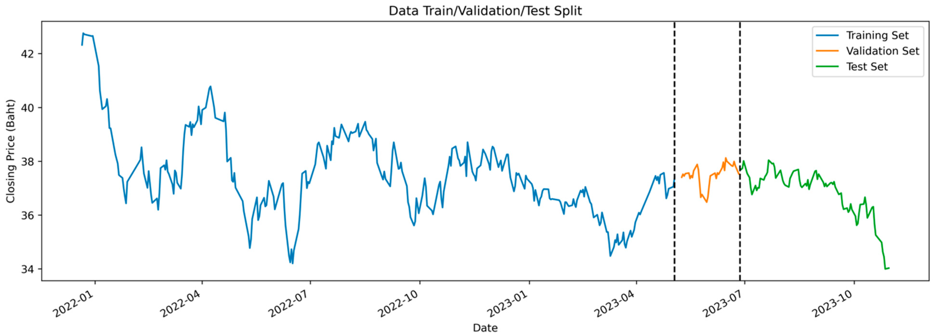
3.1. Data Collection and Descriptive Statistics

In this study, the price trading data of the Bualuang Global Health Care (BCARE) fund were selected for analysis. This fund invests solely in the feeder fund Wellington Global Health Care Equity Fund USD D Ac, which focuses on four subsectors: Major Pharmaceuticals, Biotechnology and Specialty Pharmaceuticals, Medical Products, and Health Services. The trading data of BCARE include daily closing prices, timestamped at the end of each trading day. The dataset spans from 21 December 2021, which corresponds to the date Thailand completed the administration of 100 million COVID-19 vaccine doses, to 30 October 2023, totaling 402 data points.

The dataset is divided into three segments: Training Data, Validation Data, and Test Data. Training Data and Validation Data combined constitute 80% of the dataset, with the remaining 20% designated as Test Data, resulting in 321 data points for Training and Validation, and 81 data points for Test Data. These segments are further divided at a 90:10 ratio, yielding 288 data points for Training Data and 33 for Validation Data from the initial 321. Figure 1 illustrates the dataset, showing the BCARE fund’s closing price in Thai Baht over the study period.

In the part on external factors, this study has selectively chosen factors expected to impact the prices of mutual funds in the healthcare sector. General external influences encompass the SET50 Index, representing the top 50 companies of Thailand by average daily market capitalization, monthly inflation rates (Panigrahi et al. 2019; Cheng and Dewi 2020), the Consumer Confidence Index on a monthly basis (Bolaman and EVRİM 2014), quarterly GDP growth rates (Gyamfi Gyimah et al. 2021), and the exchange rate between the Thai Baht and the US Dollar (Jasra et al. 2012; Wong 2022). Moreover, specific factors tailored to healthcare sector funds include the monthly Consumer Price Index (Subhani et al. 2010 ; Jasra et al. 2012) for Health Care and Personal Care Services, along with the Dow Jones U.S. Health Care Index (Lin 2018). This comprehensive selection incorporates a total of 7 external factors in the analytical framework.

In the section on internal factors, this study leverages historical daily price data of the top 5 holdings within the Wellington Global Health Care Equity Fund USD D Ac. These holdings consist of UnitedHealth Group Incorporated (UNH), Eli Lilly and Company (LLY), AstraZeneca PLC (AZN), Pfizer Inc. (PFE), and Danaher Corporation (DHR). A total of 12 factors (X₁, X₂, X₃, …, X₁₁, X₁₂) encompass both internal and external variables, with variable y representing the BCARE mutual fund price.

The training dataset encompasses the data utilized to facilitate the model’s exposure and learning process. Subsequently, the validation dataset serves the purpose of evaluating metrics subsequent to the model’s training phase, thereby assessing its performance and ascertaining optimal hyperparameters. Conversely, the test dataset is employed to appraise the model’s efficacy in handling previously unseen data, thereby juxtaposing its predictions against actual values. In the context of this investigation, all 12 factors were employed for training purposes, with the model endeavoring to predict the variable ‘y’, denoting the price of the BCARE fund in Thai Baht. It is imperative to underscore that the prognosticated values within this study have undergone normalization. Detailed statistical insights and supplementary elucidations pertaining to each factor are delineated in

Table 1. Statistical information and additional explanations for each factor.

Factors	Mean	Maximum	Minimum	SD	Description of Each Factor
BCARE (THB)	37.340	42.762	34.002	1.373	The historical data for the fund’s prices, denoted as the variable ‘y’ for prediction by the model, are available on a daily basis and are stated in Thai Baht.
UNH (USD)	500.471	555.15	447.75	24.201	The historical stock price data for UnitedHealth Group Incorporated, which holds the top-ranking position within the fund’s portfolio, are provided on a daily basis and are denominated in US dollars.
LLY (USD)	369.611	616.64	234.69	96.155	The historical stock price data for Eli Lilly and Company, the asset ranked second within the fund’s portfolio, are provided on a daily basis and are denominated in US dollars.
AZN (USD)	10,593.664	12294	8282	905.072	The historical stock price data for AstraZeneca PLC, the asset ranked third within the fund’s portfolio, are available on a daily basis and are denominated in US dollars.
PFE (USD)	44.538	59.55	30.11	6.968	The historical stock price data for Pfizer Inc., which is the fourth-ranked asset held within the fund, are provided on a daily basis and are denominated in US dollars.
DHR (USD)	247.868	328.47	185.1	30.178	The historical stock price data for Danaher Corporation, the asset ranked fifth within the fund’s holdings, are available on a daily basis and are denominated in US dollars.
SET50 Index	965.682	1035.94	846.89	35.164	Index data referencing the top 50 highest-valued Thai stocks in the securities market, computed as a daily index.
US Dollars Exchange Rate (THB)	34.887	38.24	32.1	1.377	Daily exchange rate records detailing the conversion rate from US dollars to Thai Baht.
Dow Jones U.S. Health Care Index	1398.889	1540.53	1271.73	45.249	A market capitalization-weighted index that tracks the performance of the healthcare sector in the United States, presented on a daily basis.
Consumer Confidence Index	49.879	56.6	43.8	4.391	An economic indicator gauging consumer confidence and overall economic sentiment, including financial conditions. These data are reported on a monthly frequency.
Consumer Price Index for Health Care and Personal Care Services	102.345	103.6	100.71	0.948	The retail price index, which measures alterations in the prices of goods and services in equivalent quantities over a specified period, relative to the prices of the same commodities in the base year. This index specifically focuses on changes in the prices of medical treatment and services within the country. Monthly data are provided.
Inflation Rate	3.915	7.86	−0.31	2.691	The consumer price index, which quantifies the percentage increase in the general price level of goods and services within an economy over a specific period, reflecting the erosion of purchasing power of a currency. Monthly data are available.
Gross Domestic Product (GDP)	2.359	4.5	1.4	0.984	Gross Domestic Product (GDP), denoting the total monetary value of all finished goods and services produced within a nation’s borders during a particular timeframe. This dataset is presented on a quarterly basis.

.

Figure 2 depicts the model-building procedure, which commences with data preprocessing to organize them for analysis. Subsequent to preprocessing, the data undergo normalization to ensure consistent scaling. Dimensionality reduction through PCA is then implemented to reduce data size and eliminate noise. The data are subsequently partitioned into training, validation, and test sets, specifically tailored for the LSTM model, whereas for the MLR model, it is divided into training and test sets at an 80:20 ratio. The ensuing steps entail training the data, fine-tuning hyperparameters using the validation set, and ultimately assessing the model’s performance against the test set. The portions of X Test and y Test, which are segregated, represent out-of-sample data since they were not utilized in the model training process. This indicates that the model has not been exposed to or learned from this dataset previously. These segments are exclusively reserved for evaluating the performance of the trained and developed model.

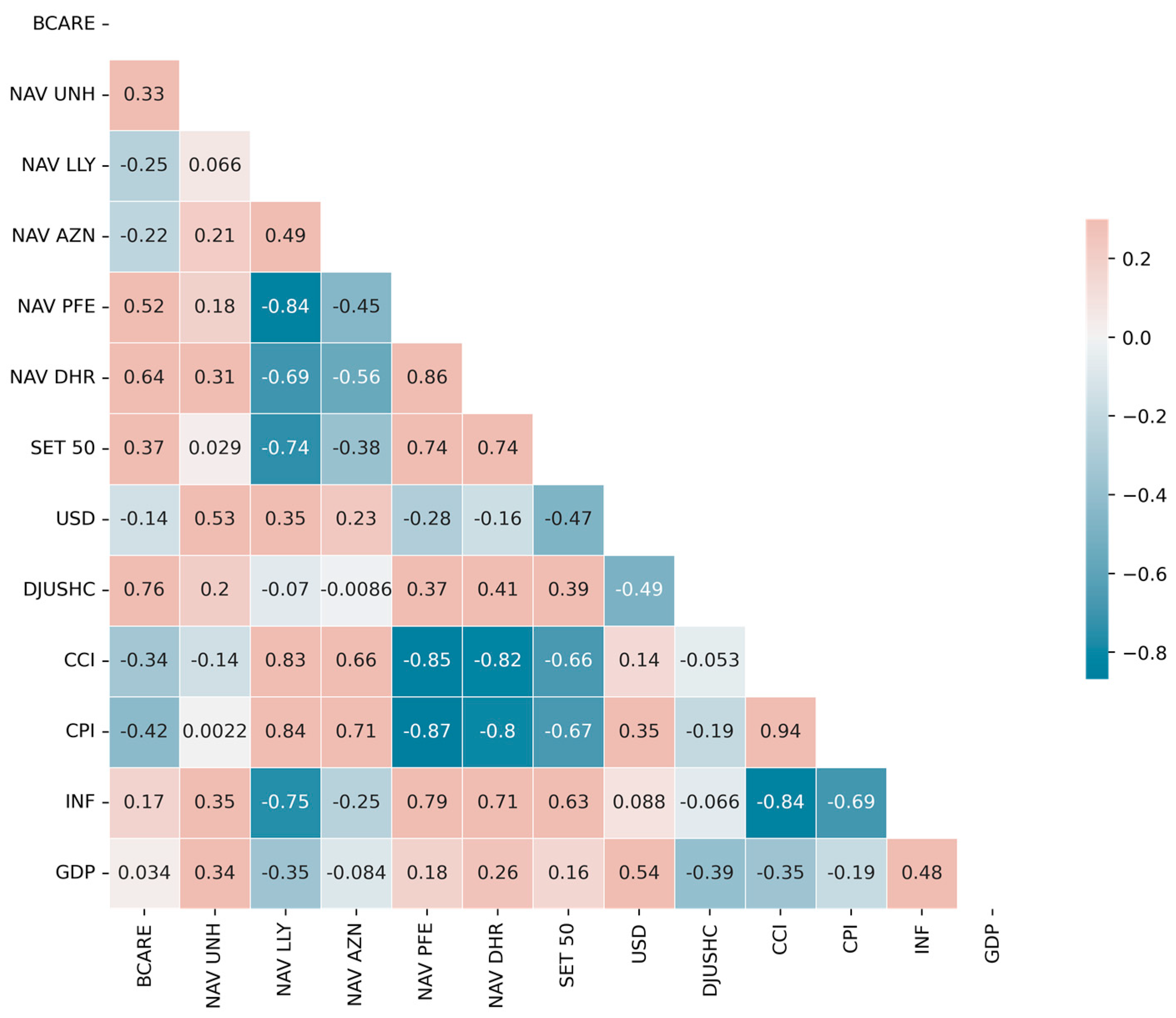
3.2. Principal Component Analysis

Principal Component Analysis (PCA) is a technique for reducing the dimensionality of data to facilitate analysis and conserve resources during model training. PCA achieves this reduction by projecting data vectors onto new axes called principal components. These components are chosen based on the variance observed along each axis. The PCA process involves three main steps (Jolliffe and Cadima 2016).

The first step is to compute the covariance matrix ($C$). The covariance matrix captures the relationships between the different features in the dataset, providing insights into how they vary together. This matrix is a critical input for the subsequent steps of PCA and is represented by Equations (1) and (2).

$$\mu =\frac{1}{N}{\sum }_{i=1}^N{X}_i$$

(1)

$$C=\frac{1}{N}{\sum }_{i=1}^N{(X}_i-\mu ){{(X}_i-\mu )}^T$$

(2)

where $N$ is the total number of data points, $X_i$ represents the data matrix, where each row corresponds to a data point, and $T$ denotes the transpose operation.

The second step involves finding the eigenvalue ($\lambda$) and eigenvector ($V$), both of which are components of the principal component and can be obtained from Equations (3) and (4).

$$Ax=b$$

(3)

where $A$ is the transformation matrix or covariance matrix, $x$ is the original vector, and $b$ is the transformed vector.

$$Ax=\lambda x$$

(4)

where $x$ is the eigenvector and $\lambda$ is the eigenvalue.

The third step involves finding the weight vector ($W$) for each data point by projecting $X_i$ onto the principal component axes ($V_1,V_2,\dots ,V_N$). The formula is presented in Equations (5) and (6).

$$W_k=V_k^T\left(X-\mu \right) ; k=1,\dots ,N$$

(5)

$$W^T=[W_1,W_2,\dots ,W_N]$$

(6)

The results obtained from PCA analysis lead to the removal of less significant data, resulting in eigenvalues and eigenvectors. These two sets of data have corresponding relationships. When sorting eigenvalues in descending order, lower eigenvalues indicate less significant data.

3.3. Multiple Linear Regression

Multiple Linear Regression (MLR) involves data analysis to examine the relationship between a dependent variable ($y_i$) and multiple independent variables ${(X}_i)$. It differs from Simple Linear Regression (SLR) in that MLR investigates relationships with more than one independent variable (Slinker and Glantz 1988). When there are k independent variables for a dependent variable, the MLR is presented in Equation (7).

$$y_i={\beta }_0+{\beta }_1{X}_{i,1}+{\beta }_2{X}_{i,2}+\dots +{\beta }_k{X}_{i,k}+{\epsilon }_i$$

(7)

where $y_i$ is the dependent variables, ${\beta }_0$ is the intercept, $X_{i,k}$ is the independent variables, ${\beta }_k$ is the vector of slope, and ${\epsilon }_i$ is the random measured errors.

In the context of forecasting, especially within a time-series framework, the integration of a dynamic model incorporating lagged terms is imperative to capture temporal dependencies and enable accurate prediction. The MLR equation utilized for forecasting purposes is delineated in Equation (8).

$$Y_t={\beta }_0+{\beta }_1{X}_{1,t}+{\beta }_2{X}_{2,t}+\dots +{\beta }_k{X}_{k,t}+{{\gamma }_1{Y}_{t-1}+{\gamma }_2{Y}_{t-2}+\dots +{\gamma }_p{Y}_{t-p}+\epsilon }_t$$

(8)

where $Y_t$ denotes the dependent variable at time t, while $Y_{t-1},Y_{t-2},\dots ,Y_{t-p}$ represent lagged values of the dependent variable up to p time periods prior. The coefficients ${\gamma }_1, {\gamma }_2,\dots ,{\gamma }_p$ correspond to the respective lagged terms.

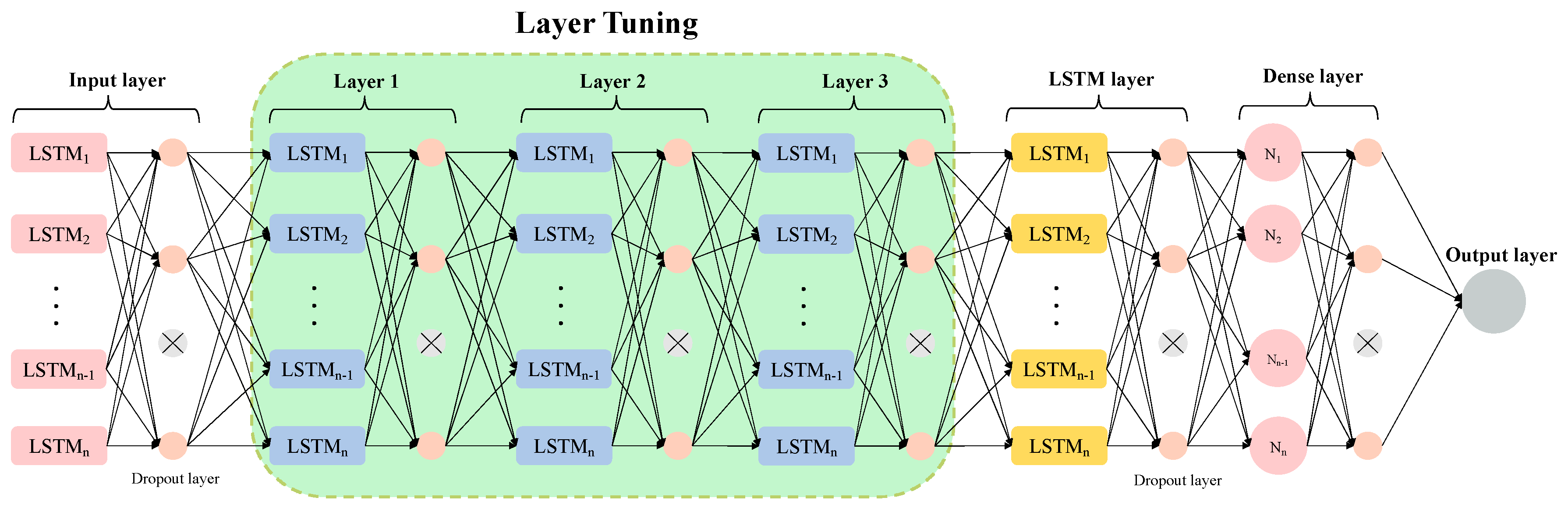
3.4. Long Short-Term Memory

Long Short-Term Memory (LSTM) constitutes a variant of Recurrent Neural Network (RNN) architecture, conceived to offer heightened stability and efficacy (Hochreiter and Schmidhuber 1997). Notably, LSTM possesses the inherent capability to maintain the state or memory of individual nodes, thereby facilitating the retention of data origins and the retrieval of preceding values during backward temporal traversals. A distinguishing characteristic of LSTM lies in its incorporation of specialized gating mechanisms that regulate the flow of information into each node. These gating mechanisms include the Forget Gate Layer, Input Gate Layer, and Output Gate Layer, collectively facilitating nuanced information management within the network. The mathematical expressions governing the operations of each gate are explicated in Equations (9) and (11).

The forget gate layer

$$f_t=\sigma (W_f.\left[h_{t-1},x_t\right]+b_f)$$

(9)

The input gate layer

$$i_t=\sigma (W_i.\left[h_{t-1},x_t\right]+b_i)$$

(10)

The output gate layer

$$o_t=\sigma (W_o.\left[h_{t-1},x_t\right]+b_o)$$

(11)

where $\sigma$ is sigmoid, $W_x$ is the neuron gate ($x$) weight, $h_{t-1}$ is the result of the preceding LSTM block, $X_t$ is the input, and $b_x$ is bias.

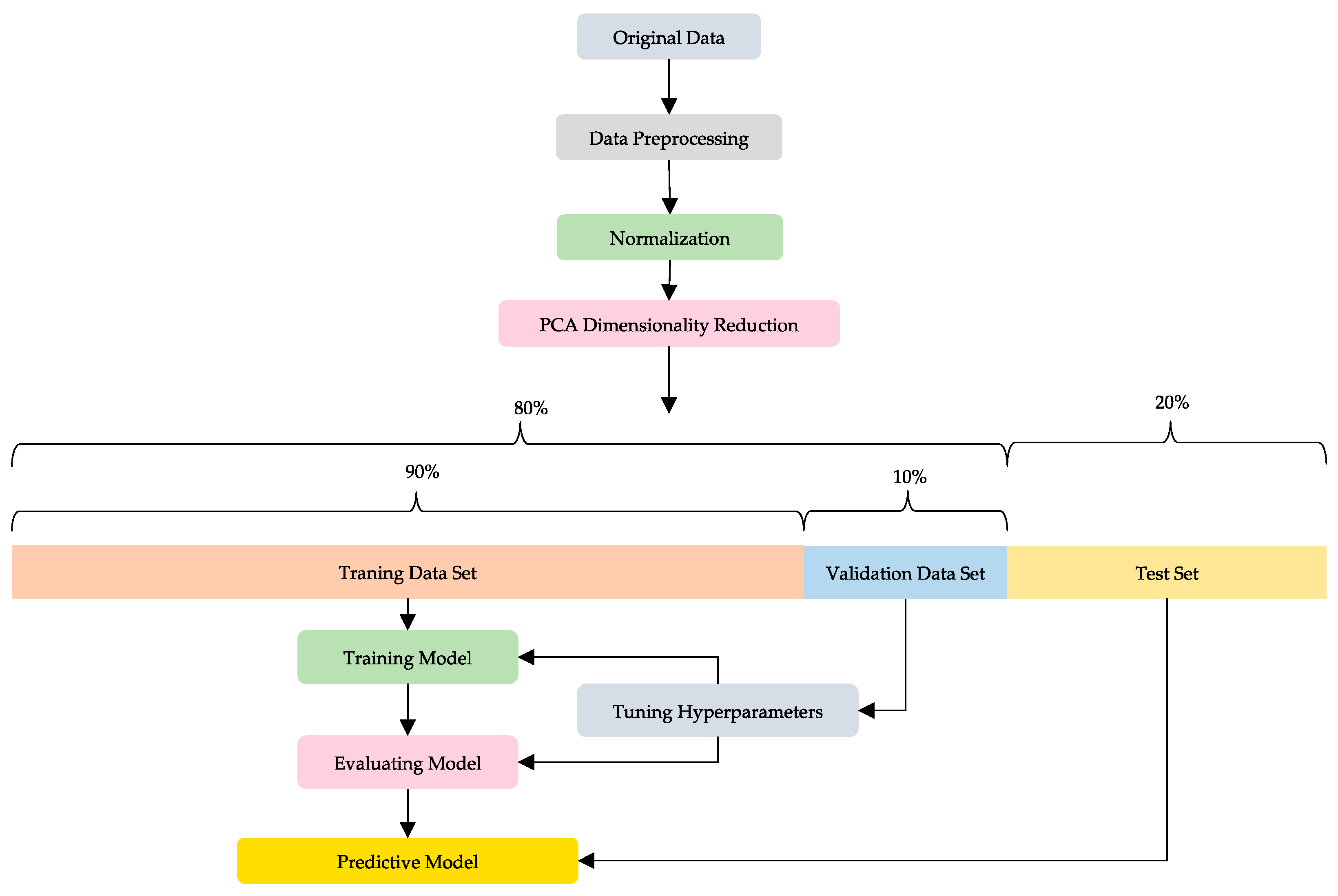
3.5. Data Preprocessing

In data processing, we often deal with different types of information that might have varying scales. Normalization and standardization are crucial steps in handling this diversity. They help ensure that all the data are on a similar scale, making them easier to compare and analyze. This is especially useful when dealing with variables that have widely different ranges, as these techniques ensure fair and consistent treatment across the board.

3.5.1. Normalization

Normalization is a method that adjusts data so that they fall within a scale of 0 to 1. It does this by subtracting the smallest value from each data point and then dividing it by the range of values (the difference between the maximum and minimum), as illustrated in Equation (12).

$$X_{scaled}=\frac{x-x_{min}}{x_{max}-x_{min}}$$

(12)

where $X_{scaled}$ is the normalized value, $x$ is the original value, $x_{min}$ is the minimum value of the features, and $x_{max}$ is the maximum value of the features.

3.5.2. Standardization

Standardization is a process that makes data have a mean of 0 and a standard deviation of 1. It achieves this by subtracting the mean from each data point and then dividing the result by the standard deviation, as illustrated in Equation (13).

$$Z=\frac{x-\mu }{\sigma }$$

(13)

where Z is the standardized value, $x$ is the original value, $\mu$ is the average value of the features, and $\sigma$ is the standard deviation of the features.

3.6. Performance Metrics

This study utilized evaluation metrics, including Root-Mean-Squared Error (RMSE), Mean-Squared Error (MSE), and Mean Absolute Error (MAE), to compare the performance of the LSTM mutual fund prediction model and assess its effectiveness. All of the performance metrics are mathematically represented in Equations (14)–(16).

$$RMSE=\sqrt{{\sum }_{i=1}^n\frac{{({\widehat{y}}_i-y_i)}^2}{n}}$$

(14)

$$MSE={RMSE}^2$$

(15)

$$MAE=\frac{1}{n} {\sum }_{i=1}^n|y_i-{\widehat{y}}_i|$$

(16)

where $y_i$ denotes actual value, ${\widehat{y}}_i$ denotes predicted value, and ${\overline{y}}_i$ denotes the mean of $y_i$ value.

3.7. Diebold–Mariano Test

The Diebold–Mariano test serves as a statistical method for comparing the forecast accuracy between two models, designated as Model 1 and Model 2 (Diebold and Mariano 1995). The test statistic, denoted as DM, is calculated as the difference in mean-squared forecast errors (DMSFE) divided by the standard error of the differences, as depicted in Equation (17).

$$DM=\frac{DMSFE}{\sqrt{\frac{1}{T}{\sum }_{t=1}^T({\frac{e_{1t}-e_{2t}}{T})}^2}}$$

(17)

where $e_{1t}$ and $e_{2t}$ represent the forecast errors of Model 1 and Model 2, respectively, at time t, while $T$ signifies the total number of observations. This test aims to ascertain whether there exists a statistically significant distinction in forecast accuracy between the two models.

When the Diebold–Mariano (DM) statistic significantly deviates from zero, it signifies that one model demonstrates superior performance compared to the other. The corresponding p-value offers insight into the significance level of this discrepancy, thereby facilitating informed decision-making regarding model selection.

4. Results and Discussion

4.1. Dimensionality Reduction

Principal Component Analysis (PCA) is a method used to reduce the dimensionality of large datasets by transforming numerous features or X values into a smaller set that still retains the essential information of the dataset (Jolliffe and Cadima 2016). This is particularly useful for datasets with a large number of features, as it simplifies exploration and visualization, making data analysis more efficient. Additionally, working with a smaller dataset helps avoid issues like overfitting, where models may try to capture noise in the data, leading to improved model generalization.

In the initial step of PCA, the process begins with standardizing the entire dataset to ensure that each feature has an equal impact on data analysis. Subsequently, the covariance matrix is computed, representing the covariance values between all possible pairs of features in the dataset. A positive covariance indicates a direct relationship, implying that the variables increase or decrease together (correlated). Conversely, a negative covariance signifies an inverse relationship, suggesting that when one variable increases, the other decreases (inversely correlated). This covariance matrix provides insights into the relationships among different features in the dataset.

In the final step, the covariance matrix is used to calculate eigenvectors and arrange them in descending order based on their corresponding eigenvalues. This process allows us to identify principal components in order of importance. At this stage, a choice can be made to either retain all components or discard less significant ones (those with lower eigenvalues).

Table 2. The eigenvalues for each component and cumulative values.

Principal Component	Explained Variance	Explained Variance Ratio	Cumulative Explained Variance Ratio
1	6.27746	0.52182	0.52182
2	2.37639	0.19754	0.71936
3	1.46909	0.12211	0.84147
4	0.76288	0.06341	0.90489
5	0.44540	0.03702	0.94191
6	0.24519	0.02038	0.96230
7	0.17680	0.01469	0.97699
8	0.09612	0.00799	0.98498
9	0.07860	0.00653	0.99152
10	0.05038	0.00418	0.99570
11	0.03661	0.00304	0.99875
12	0.01501	0.00124	1.00000

presents the eigenvalues for each component and cumulative values, illustrating how well the selected components cover the variance of the entire dataset. It is evident that choosing to retain the first 6 components covers approximately 96.23% of the dataset’s variance, exceeding the 95% threshold. Thus, this study opted to reduce the dimensionality of features to only 6 dimensions. However, it is crucial to note that this dimensionality reduction does not involve discarding data but rather constructing new features that effectively summarize the existing information.

Table 3. The covariance values for original features with the newly created 6 components.

Factors	PC1	PC2	PC3	PC4	PC5	PC6
UNH	−0.05395	0.39391	−0.58507	0.2138	0.11052	−0.0905
LLY	0.35898	0.01049	−0.17060	0.31135	0.02323	−0.33053
AZN	0.24575	0.11064	−0.36409	−0.67845	0.22114	0.18960
PFE	−0.37475	−0.02941	−0.13328	−0.06051	0.23523	0.27940
DHR	−0.36112	0.02441	−0.20098	0.22107	−0.13946	−0.11840
SET50	−0.32792	−0.13587	−0.11733	−0.32707	−0.38088	−0.65376
USD	0.11597	0.58036	−0.03926	0.25511	0.048396	−0.05818
DJUSHC	−0.10143	−0.35613	−0.60917	0.13878	−0.27575	0.31157
CCI Index	0.37847	−0.09041	−0.11985	−0.13022	−0.20164	0.01365
CPI Index	0.37481	0.06522	−0.13017	−0.16696	−0.16590	−0.24640
Inflation Rate	−0.32748	0.26784	−0.03579	−0.28068	0.36433	−0.2438
GDP Growth	−0.12131	0.51451	0.13735	−0.17183	−0.6627	0.32604

displays the covariance values for all 12 original features and their relationships with the newly created 6 components.

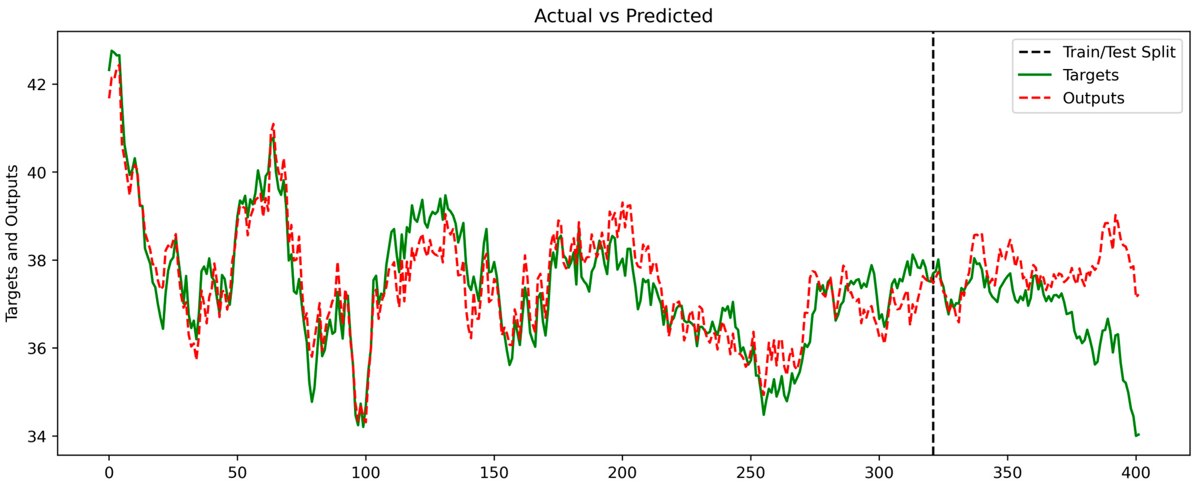
4.2. MLR Prediction Results

In the context of MLR, generally, it is necessary to satisfy the assumptions of multiple linear regression before performing MLR to ensure reliable results. One of these assumptions is the absence of multicollinearity, meaning that none of the predictor variables should be highly correlated with each other. Conventionally, an analysis of correlation values extracted from the correlation matrix, depicted in Figure 3, is conducted to assess the relationships between the dependent and independent variables. The correlation values range from -1 to 1, and a correlation exceeding 0.8 indicates a high level of correlation between variables (Berry and Feldman 1985). If such multicollinearity exists, it can impact the accuracy of various statistical estimates.

However, this study has proposed the use of all 12 features in creating MLR. The data are divided into Training Data and Test Data in an 80:20 ratio, with no separate Validation Data. The outcomes of employing MLR for prediction are delineated in

Table 4. RMSE and MSE for MLR prediction mutual fund prices.

Training Set		Testing Set
RMSE Train	MSE Train	RMSE Test	MSE Test
0.5585	0.3119	1.4158	2.0046

and Figure 4. Within the y-axis section, representing targets and output, the graph illustrates the model’s predicted prices compared with the actual values, while the x-axis denotes the total number of data points. It is observed that the MLR demonstrates efficiency in predicting the Train dataset interval with an MSE of 0.3119 and RMSE of 0.5585. However, the model tends to exhibit characteristics of attempting to fit noise data excessively during this interval. Consequently, during the Test dataset interval, MLR predicts results with significantly reduced effectiveness, as evidenced by an MSE of 2.0046 and RMSE of 1.4158. The outcomes of utilizing MLR reveal a notable issue of overfitting, signifying a scenario where the model is trained to be overly complex and, consequently, cannot be effectively applied when encountering new data. The performance metrics for MLR prediction include an RMSE Overall of 0.8081 and MSE Overall of 0.6530. These findings emphasize the challenge of overfitting in the MLR model, illuminating its constraints when encountering unfamiliar datasets.

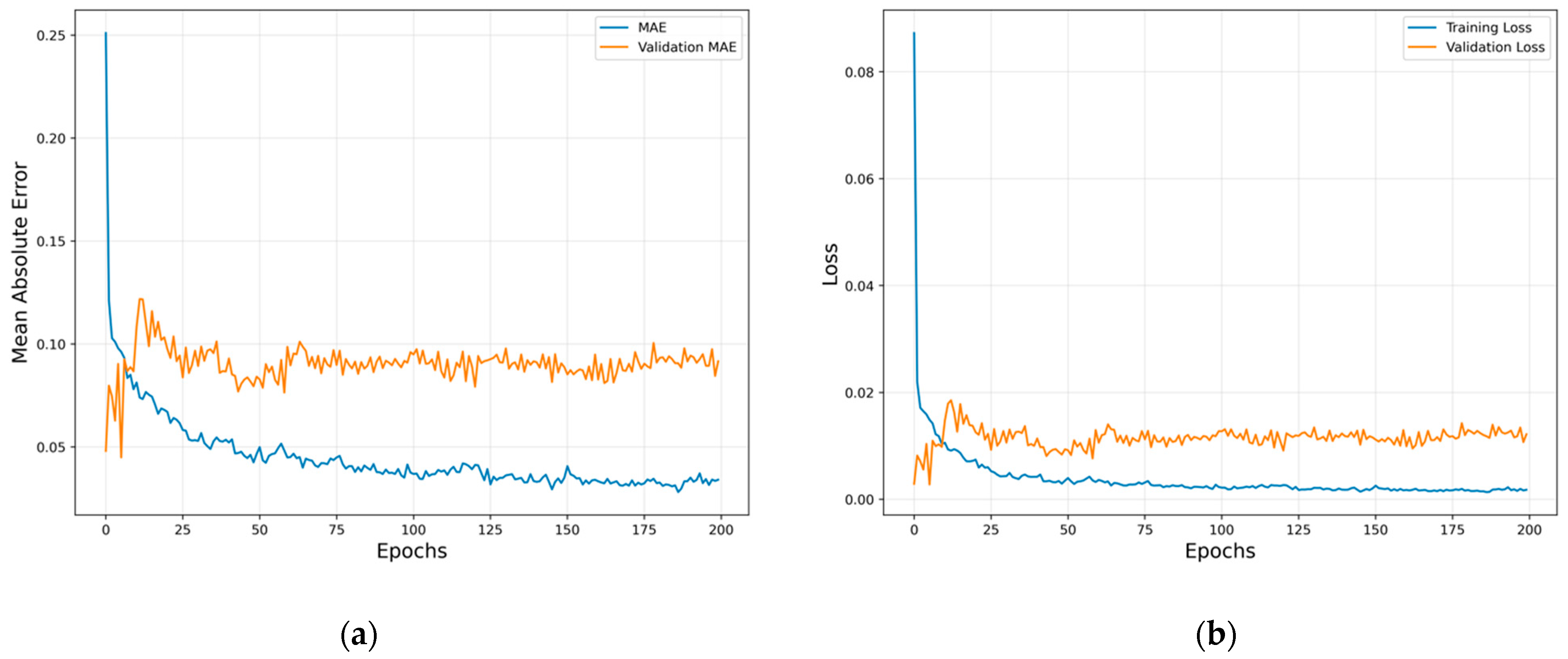
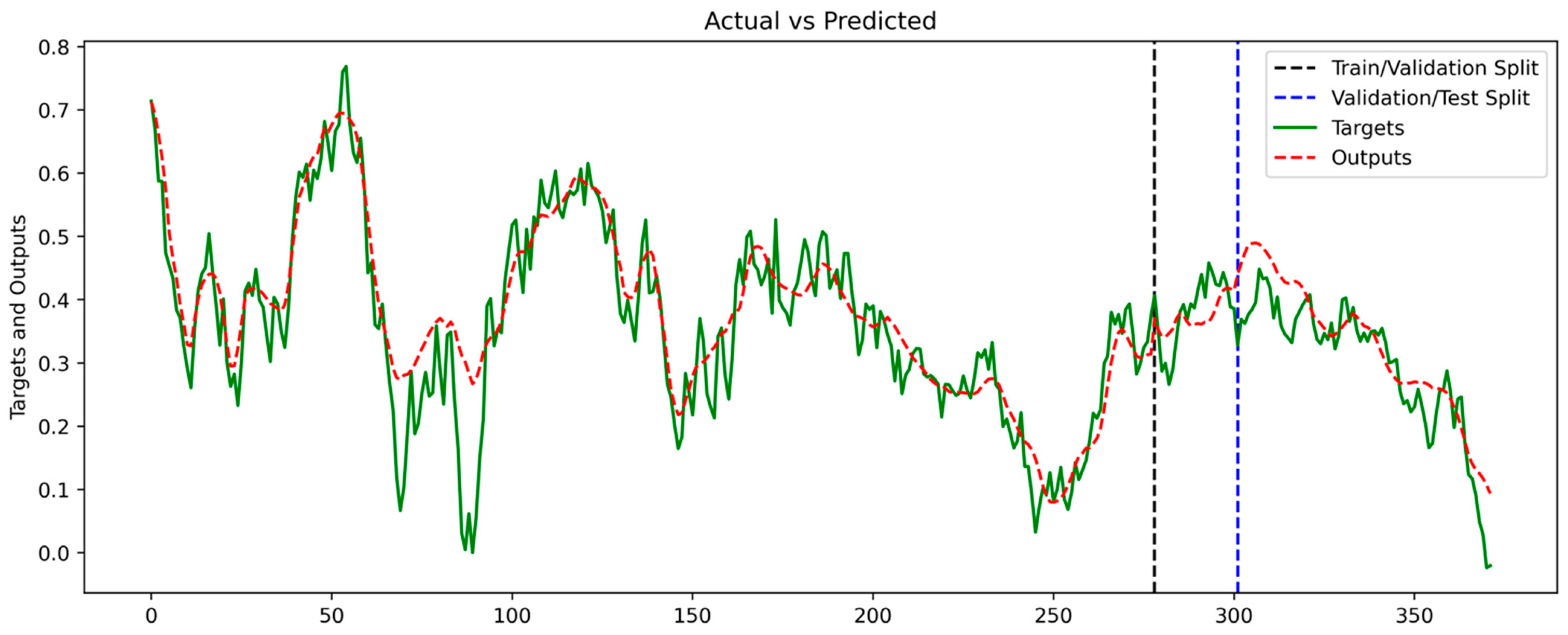
4.3. LSTM Prediction Results

In the section on model tuning, this study introduced the tuning of the number of neurons and hidden layers. Figure 5 illustrates the model architecture designed for this purpose. The tuning focused on layers 1, 2, and 3, with variations in the number of neurons. Furthermore, LSTM layers and Dense layers were added after the initial tuning of the specified layers. The number of neurons considered for tuning included 32, 64, 128, and 256. The input data provided to the input layer encompass all 12 factors mentioned earlier. The optimized number of neurons is implemented across all layers, including the input layer, as illustrated in Figure 5, with the exception of the output layer, which consists of only one neuron. Moreover, we have established the duration of observations considered by the model when learning a time series, commonly referred to as the window size. This determination was influenced by the relatively restricted number of price data points available post-COVID-19. In this investigation, various window sizes were tested, namely 10, 12, 15, and 20 days. The batch size was set at 64, and epochs were configured to 40. To mitigate overfitting, Dropout layers were incorporated after the Input Layer and every Hidden Layer, each with a dropout rate of 0.2.

Table 5. Prediction results under different number of neurons, hidden layers, and window sizes.

Window Size	LSTM Layer 1	LSTM Layer 2	LSTM Layer 3	Number of Neurons	MSE Train	MSE Validation
10 days	1	1	1	256	0.00301	0.00942
	1	0	1	256	0.00361	0.01004
	1	1	0	256	0.00619	0.01089
	1	1	0	32	0.01047	0.01149
	1	1	1	64	0.00383	0.01175
	0	1	1	64	0.00379	0.01199
	0	1	1	256	0.00534	0.01210
	0	0	1	256	0.00372	0.01246
	0	1	0	2256	0.00310	0.01275
	0	1	1	32	0.00459	0.01426
12 days	1	1	1	128	0.00347	0.00954
	0	1	1	256	0.00370	0.01039
	1	1	0	256	0.00306	0.01288
	1	1	1	256	0.00302	0.01298
	1	0	1	256	0.00380	0.01328
	1	1	1	32	0.00502	0.01363
	1	1	1	64	0.00369	0.01440
	0	0	1	256	0.00613	0.01512
	0	1	0	64	0.00443	0.01523
	1	0	0	128	0.00537	0.01579
15 days	1	1	1	128	0.00409	0.01394
	1	1	1	256	0.00452	0.01467
	1	1	1	64	0.00353	0.01623
	1	1	0	256	0.00380	0.01684
	1	0	1	256	0.00470	0.01734
	0	0	1	256	0.00375	0.01774
	1	1	0	32	0.00428	0.01803
	0	0	0	256	0.00421	0.01954
	0	1	1	64	0.00315	0.01978
	1	1	1	32	0.00421	0.02021
20 days	1	1	1	256	0.00329	0.01175
	1	1	0	256	0.00397	0.01207
	0	1	1	256	0.00322	0.01450
	1	1	1	128	0.00293	0.01451
	1	0	1	256	0.00445	0.01461
	1	1	1	64	0.00338	0.01552
	0	1	0	256	0.00517	0.01670
	1	0	0	256	0.00516	0.01721
	0	0	1	256	0.00465	0.01816
	0	0	0	256	0.00416	0.01876

presents the top 10 outcomes from a pool of 32 distinct configurations, showcasing the lowest Mean-Squared Error (MSE) values achieved through the tuning of neuron numbers and hidden layers across various window sizes. Notably, with a window size of 10 days, the recorded performance metrics reveal an MSE of 0.00301 for the training dataset and an MSE of 0.00942 for the validation dataset.

The Learning Curve is a graph illustrating the performance of the model on both Training Data and Validation Data, measured after the hyperparameter tuning process. It aims to identify whether the model suffers from issues like overfitting or underfitting (Anzanello and Fogliatto 2011). The x-axis represents the number of training cycles (Epochs), while the y-axis shows the model’s performance. Figure 6a illustrates both the Mean Absolute Error (MAE) and Training Loss. After obtaining the optimal hyperparameters, they exhibit a continuous decreasing trend until approximately 25 epochs, where they stabilize. Similarly in Figure 6b, Validation MAE and Validation Loss increase initially and then stabilize as the model is trained for more epochs. The observed pattern in the Learning Curve indicates a well-fitting model, demonstrating good learning capabilities and the ability to generalize to unseen data.

Table 6. RMSE and MSE for LSTM prediction mutual fund prices.

Training Set		Validation Set		Testing Set
RMSE Train	MSE Train	RMSE Validation	MSE Validation	RMSE Test	MSE Test
0.0617	0.0038	0.0458	0.0021	0.0547	0.0030

shows the results obtained from the predictions. The y-axis represents both targets and output, denoting the prices predicted by the model in comparison to the actual values. Meanwhile, the x-axis indicates the total number of data points. It is important to note that the values on the y-axis represent prices after normalization, scaled between 0 and 1. It can be observed that the model learns and predicts well within the range of the training data, with an RMSE of 0.0617 and MSE of 0.0038. The use of a 10-day window size for predicting future prices allows the model to forecast trends rather than capturing noise in the data. The model’s accuracy on the validation set slightly decreased from the training phase, yielding an RMSE of 0.0458 and MSE of 0.0021. Conversely, during the testing phase, there was an increase in error metrics compared to before, with an RMSE of 0.0547 and MSE of 0.0030. The model accurately predicts a significant downward trend in future data, consistent with the actual test data showing a decline in fund prices as illustrated in Figure 7. Overall, this model produces an RMSE Overall of 0.0596 and MSE overall of 0.0035.

4.4. Diebold–Mariano Test

The Diebold–Mariano test was utilized to evaluate whether there is a statistically significant difference in forecast accuracy between LSTM and MLR, as detailed in

Table 7. The results of the Diebold–Mariano Test.

	Diebold–Mariano Test Statistic	p-Value
DM test based on MLR and LSTM	−2.2334	0.02867

. In this analysis, the Diebold–Mariano test statistic was computed as −2.2334. The negative value indicates the difference in mean-squared forecast errors between the two models, adjusted for the variance of the differences, suggesting that LSTM demonstrates a lower mean-squared forecast error compared to MLR. Regarding the p-value, it was found to be 0.02867. This value represents the probability of observing a test statistic as extreme as the calculated one under the assumption that the null hypothesis is true. With a p-value less than 0.05, the observed difference is deemed statistically significant in this study.

In the comparative analysis with previous studies on forecasting healthcare securities, as presented in

Table 8. Comparison of healthcare securities prediction performances with the literature.

References	Subject	Description of Data	Model	RMSE	Accuracy
Ahmed et al. (2022)	The paper incorporates various machine learning algorithms, including SVM, reinforcement learning, ANN, and RNN, to forecast stock prices within the healthcare sector.	The dataset encompasses healthcare stock price data spanning the years 2016 to 2019, comprising fields such as opening and closing prices, alongside features such as price volatility and momentum.	Linear Regression	0.080	-
			RNN with GRU	0.051	-
			SVM	0.079	-
			Random Forest	0.065	-
Jariyapan et al. (2022)	Supervised learning algorithms such as Linear Discriminant Analysis (LDA), k-Nearest Neighbors (kNN), and Support Vector Machine (SVM) are employed to explore the cycle regimes of healthcare stocks over the next five years.	Monthly stock price data from 2015 to 2020 for five healthcare sector stock price indexes, specifically sourced from the Nasdaq index, were utilized in the paper.	LDA	-	0.8138
			k-NN	-	0.5223
			SVM	-	0.7847
Chatterjee et al. (2021)	Six models are developed, integrating time series, econometric, and learning-based techniques, specifically tailored for stock price prediction across three major sectors, with a particular focus on the healthcare sector.	Data pertaining to SUN Pharmaceuticals, covering the period from January 2004 to December 2019, were employed in the study.	Holt–Winters	0.056	-
			ARIMA	0.020	-
			Random Forest	0.009	-
			MARS	0.017	-
			RNN	0.0209	-
			LSTM	0.022	-
Mokhlis et al. (2021)	Time series models such as ARIMA, GARCH, and TGARCH are utilized to predict the IHH stock price, and their performances are evaluated using RMSE.	The paper leverages daily data of the IHH stock price to forecast its future trends and volatility, encompassing the period from September 2015 to September 2021.	ARIMA (4,1,5) -GARCH (1,1)	0.02289412	-
			ARIMA (4,1,5) -TGARCH (1,1)	0.02289852	-

, which are relatively limited in quantity, this research demonstrates a favorable RMSE value of 0.0547. This result surpasses the performance of Linear Regression, SVM, and Random Forest models, and in comparison to the LSTM model, the findings are closely aligned. However, it is noteworthy that the RMSE obtained in this study, at 0.0547, is slightly higher than the RMSE reported in the previous study by Ahmed et al. (2022), where the RMSE was 0.051. Nevertheless, it is important to acknowledge that the results of this research fall short compared to the studies conducted by Chatterjee et al. (2021) and Mokhlis et al. (2021).

In this study, our aim is to demonstrate the utilization of diverse influencing factors from economic, industrial, and corporate contexts to forecast future price trends in the healthcare industry. The results obtained indicate an enhancement over using general historical trading data in certain machine learning models (Ahmed et al. 2022). Although the outcomes may not surpass those of previous studies (Chatterjee et al. 2021; Mokhlis et al. 2021), we introduce a novel data approach that extends beyond solely relying on past securities trading data. By examining the future price prediction of healthcare mutual funds using various external factors, the results closely align with historical data, suggesting the potential application of these external factors in forecasting securities across other sectors. It is important to note that these factors may vary across different industries. Transforming diverse data into analyzable formats could facilitate the integration of these factors into accurate predictive models, thereby contributing to improved forecasting across various industries.

Regarding the limitations of this study, it is possible that there are factors and data points overlooked beyond what has been presented, potentially extending beyond the scope analyzed in this study. These could encompass additional economic indicators, insightful data within the healthcare industry, or other contexts that can be quantified for analysis. It is advisable to consider incorporating such data to enhance the comprehensiveness of the analysis. Furthermore, the combination of models has the potential to improve accuracy and mitigate risks associated with individual model limitations, ultimately leading to more reliable predictions.

In addition to the aforementioned points, there is also the issue of applying this model in practical usage. Forecasting the value of y in the actual future necessitates knowledge of the values of X in the future. Specifically, this entails knowing the values of X_t+1, X_t+2, …, X_t+n. Thus, there is a need to consider making X dynamic through a process known as rolling forecast in machine learning. This can be achieved by constructing a model from the existing X data. Such models may include regression models, time series models, machine learning algorithms, deep learning models, or other models that are suitable for the dataset to predict the values of X in the future. Subsequently, the predicted values of X are used to forecast the value of y in an LSTM model that has undergone hyperparameter tuning. However, it is imperative that the models used for predicting each X value exhibit efficacy, as the accuracy of predicting X directly influences the prediction of y.

5. Conclusions and Future Work

In conclusion, this study has presented the utilization of both internal and external factors expected to impact the prices of mutual funds in the medical business sector. These factors were used to build a model for predicting future price trends. The external factors include the SET50 Index, inflation rates, Consumer Confidence Index, GDP growth rates, exchange rates between the Thai Baht and the US Dollar, Consumer Price Index for Health Care and Personal Care Services, and Dow Jones U.S. Health Care Index. Additionally, internal factors consist of historical daily price data for the top 5 holdings: UnitedHealth Group Incorporated (UNH), Eli Lilly and Company (LLY), AstraZeneca PLC (AZN), Pfizer Inc (PFE), and Danaher Corporation (DHR), resulting in a total of 12 features. This study has presented the selection of data to cover various factors that may affect mutual fund prices in the healthcare sector only. However, in other sectors, there may be other factors affecting fund prices beyond what has been discussed in this study. Additionally, the data used are relatively limited in quantity.

This study employed PCA to reduce the dimensionality of the data, making them more manageable for faster processing and avoiding overfitting issues associated with capturing data noise. The data dimensionality was reduced from 12 features to 6 features, retaining up to 96.23 percent of the information.

In the part on MLR, its predictive performance was less effective during the testing phase. The MLR model yielded results with an RMSE Test of 1.4158 and MSE Test of 2.0046, suggesting limitations in predicting outcomes during scenarios involving unseen data.

And in the LSTM section, hyperparameter tuning was conducted, resulting in the optimal configuration of a 4-layer LSTM followed by 1 dense layer, featuring 256 neurons, a batch size of 64, 40 epochs, a dropout rate of 0.2, and a specified window size of historical data for the past 10 days. The predictive results yielded an RMSE Test of 0.0547 and MSE Test of 0.0030. In addition, an analysis utilizing the Diebold–Mariano test has shown a statistically significant difference in the prediction results between the two, with LSTM exhibiting a lower MSE than MLR. The reduction percentages for RMSE and MSE when using LSTM are approximately 96.13% and 99.85%, respectively.

This study demonstrates that utilizing both internal and external factors in conjunction with LSTM is more effective in forecasting trends in healthcare sector mutual fund prices compared to MLR. The price fluctuations in these funds are influenced by various contributing factors, and these diverse elements can be used as valuable data for constructing predictive models to anticipate future trends.

For future work, we plan to explore the application of other machine learning models such as Decision Trees, Random Forests, or Artificial Neural Networks. Additionally, we aim to investigate model combinations such as LSTM-GRU, LSTM-CNN, and LSTM-VAR. Our future plans involve expanding the findings by incorporating additional factors beyond those presented in this study and integrating them with historical trading data. This comprehensive approach will be extended to mutual funds across various sectors. Furthermore, we also contemplate applying this model for rolling forecast by constructing various models to predict the value of X, including regression models, time series models, machine learning algorithms, deep learning models, or other models suitable for the dataset. These models are employed to forecast the value of y in the future using LSTM.

References

1. Ahmed, Daiyaan, Ronhit Neema, Nishant Viswanadha, and Ramani Selvanambi. 2022. Analysis and Prediction of Healthcare Sector Stock Price Using Machine Learning Techniques: Healthcare Stock Analysis. International Journal of Information System Modeling and Design (IJISMD) 13: 1–15. [Google Scholar] [CrossRef]
2. Alnabulsi, Khalil, Emira Kozarević, and Abdelaziz Hakimi. 2023. Non-Performing Loans and Net Interest Margin in the MENA Region: Linear and Non-Linear Analyses. International Journal of Financial Studies 11: 64. [Google Scholar] [CrossRef]
3. Alzubi, Jafar, Anand Nayyar, and Akshi Kumar. 2018. Machine learning from theory to algorithms: An overview. Journal of Physics: Conference Series 1142: 012012. [Google Scholar] [CrossRef]
4. Anzanello, Michel Jose, and Flavio Sanson Fogliatto. 2011. Learning curve models and applications: Literature review and research directions. International Journal of Industrial Ergonomics 41: 573–83. [Google Scholar] [CrossRef]
5. Banegas, Ayelen, Gabriel Montes-Rojas, and Lucas Siga. 2022. The effects of US monetary policy shocks on mutual fund investing. Journal of International Money and Finance 123: 102676. [Google Scholar] [CrossRef]
6. Berry, William Dale, and Stanley Feldman. 1985. Multiple Regression in Practice. Newcastle upon Tyne: Sage. [Google Scholar]
7. Bolaman, Özge, and Pınar EVRİM. 2014. Effect of investor sentiment on stock markets. Finansal Araştırmalar ve Çalışmalar Dergisi 6: 51–64. [Google Scholar] [CrossRef]
8. Bolboacă, Roland, and Piroska Haller. 2023. Performance Analysis of Long Short-Term Memory Predictive Neural Networks on Time Series Data. Mathematics 11: 1432. [Google Scholar] [CrossRef]
9. Brogaard, Jonathan, and Abalfazl Zareei. 2023. Machine learning and the stock market. Journal of Financial and Quantitative Analysis 58: 1431–72. [Google Scholar] [CrossRef]
10. Chatterjee, Ananda, Hrisav Bhowmick, and Jaydip Sen. 2021. Stock price prediction using time series, econometric, machine learning, and deep learning models. Paper presented at the 2021 IEEE Mysore Sub Section International Conference (MysuruCon), Hassan, India, October 24–25. [Google Scholar]
11. Cheng, Leonardo, and Kartika Dewi. 2020. The effects of inflation, risk, and money supply on mutual funds performance. Journal of Applied Finance and Accounting 7: 29–34. [Google Scholar] [CrossRef]
12. Chimmula, Vinay Kumar Reddy, and Lei Zhang. 2020. Time series forecasting of COVID-19 transmission in Canada using LSTM networks. Chaos, Solitons & Fractals 135: 109864. [Google Scholar]
13. Diebold, Francis X., and Roberto S. Mariano. 1995. Comparing predictive accuracy. Journal of Business and Economic Statistics 13: 253–63. [Google Scholar]
14. Dillender, Marcus, Andrew Friedson, Cong Gian, and Kosali Simon. 2021. Is healthcare employment resilient and “recession proof”? INQUIRY: The Journal of Health Care Organization, Provision, and Financing 58: 00469580211060260. [Google Scholar]
15. Ersin, Özgür Ömer, and Melike Bildirici. 2023. Financial Volatility Modeling with the GARCH-MIDAS-LSTM Approach: The Effects of Economic Expectations, Geopolitical Risks and Industrial Production during COVID-19. Mathematics 11: 1785. [Google Scholar] [CrossRef]
16. Gu, Shihao, Bryan Kelly, and Dacheng Xiu. 2020. Empirical asset pricing via machine learning. The Review of Financial Studies 33: 2223–73. [Google Scholar] [CrossRef]
17. Gülmez, Burak. 2023. Stock price prediction with optimized deep LSTM network with artificial rabbits optimization algorithm. Expert Systems with Applications 227: 120346. [Google Scholar] [CrossRef]
18. Gyamfi Gyimah, Adjei, Bismark Addai, and George Kwasi Asamoah. 2021. Macroeconomic determinants of mutual funds performance in Ghana. Cogent Economics & Finance 9: 1913876. [Google Scholar]
19. Heshmaty, Behrooz, and Abraham Kandel. 1985. Fuzzy linear regression and its applications to forecasting in uncertain environment. Fuzzy Sets and Systems 15: 159–91. [Google Scholar] [CrossRef]
20. Hochreiter, Sepp, and Jürgen Schmidhuber. 1997. Long short-term memory. Neural Computation 9: 1735–80. [Google Scholar] [CrossRef] [PubMed]
21. Janiesch, Christian, Patrick Zschech, and Kai Heinrich. 2021. Machine learning and deep learning. Electronic Markets 31: 685–95. [Google Scholar] [CrossRef]
22. Jariyapan, Prapatchon, Jittima Singvejsakul, and Chukiat Chaiboonsri. 2022. A Machine Learning Model for Healthcare Stocks Forecasting in the US Stock Market during COVID-19 Period. Journal of Physics: Conference Series 2287: 012018. [Google Scholar] [CrossRef]
23. Jasra, Javed Mahmood, Rauf I Azam, and Muhammad Asif Khan. 2012. Impact of macroeconomic variables on stock prices: Industry level analysis. Actual Problems of Economics 134: 403–12. [Google Scholar]
24. Jolliffe, Ian T., and Jorge Cadima. 2016. Principal component analysis: A review and recent developments. Philosophical Transactions of the Royal Society A: Mathematical, Physical and Engineering Sciences 374: 20150202. [Google Scholar] [CrossRef]
25. Kang, Yushan, Jian Xing, and Shanhui Zhao. 2022. Influencing Factors of Investment for Companies. Paper presented at the 2022 7th International Conference on Financial Innovation and Economic Development (ICFIED 2022), Harbin, China, January 21–23. [Google Scholar]
26. Kittichotsatsawat, Yotsaphat, Nakorn Tippayawong, and Korrakot Yaibuathet Tippayawong. 2022. Prediction of arabica coffee production using artificial neural network and multiple linear regression techniques. Scientific Reports 12: 14488. [Google Scholar] [CrossRef]
27. Kumar, P. Rajendra, and E. Bala Krishna Manash. 2019. Deep learning: A branch of machine learning. Journal of Physics: Conference Series 1228: 012045. [Google Scholar]
28. Li, Zheming. 2020. Economic Policy Uncertainty and Mutual Fund’s Risk Adjusting Behavior in China. Modern Economy 11: 609–19. [Google Scholar] [CrossRef]
29. Lin, Eric C. 2018. The effect of Dow Jones industrial average index component changes on stock returns and trading volumes. The International Journal of Business and Finance Research 12: 81–92. [Google Scholar]
30. Mokhlis, Nur Hanis Mohd, Nur Anira Ahmad Burhan, Nur Fatin Ainsyah Roeslan, Siti Nur Aishah Zainal Moin, and Ummu Aiman Mohd Nur. 2021. Forecasting healthcare stock price using arima-garch model and its value at risk. International Journal of Business and Economy 3: 127–42. [Google Scholar]
31. Ouyang, Qi, Yongbo Lv, Jihui Ma, and Jing Li. 2020. An LSTM-based method considering history and real-time data for passenger flow prediction. Applied Sciences 10: 3788. [Google Scholar] [CrossRef]
32. Panigrahi, Ashok, Pradhum Karwa, and Pushkin Joshi. 2019. Impact of macroeconomic variables on the performance of mutual funds: A selective study. Journal of Economic Policy & Research October 15: 1–13. [Google Scholar]
33. Qureshi, Fiza, Ali M Kutan, Izlin Ismail, and Chan Sok Gee. 2017. Mutual funds and stock market volatility: An empirical analysis of Asian emerging markets. Emerging Markets Review 31: 176–92. [Google Scholar] [CrossRef]
34. Sarker, Iqbal H. 2021. Deep Learning: A Comprehensive Overview on Techniques, Taxonomy, Applications and Research Directions. SN Computer Science 2: 420. [Google Scholar] [CrossRef] [PubMed]
35. Sen, Jaydip, Sidra Mehtab, Abhishek Dutta, and Saikat Mondal. 2021. Precise stock price prediction for optimized portfolio design using an LSTM model. Paper presented at the 2021 19th OITS International Conference on Information Technology (OCIT), Bhubaneswar, India, December 16–18. [Google Scholar]
36. Shah, Jaimin, Darsh Vaidya, and Manan Shah. 2022. A comprehensive review on multiple hybrid deep learning approaches for stock prediction. Intelligent Systems with Applications 16: 200111. [Google Scholar] [CrossRef]
37. Slinker, Bryan K., and Stanton A Glantz. 1988. Multiple linear regression is a useful alternative to traditional analyses of variance. American Journal of Physiology-Regulatory, Integrative and Comparative Physiology 255: R353–R367. [Google Scholar] [CrossRef] [PubMed]
38. Sonkavde, Gaurang, Deepak Sudhakar Dharrao, Anupkumar M Bongale, Sarika T Deokate, Deepak Doreswamy, and Subraya Krishna Bhat. 2023. Forecasting stock market prices using machine learning and deep learning models: A systematic review, performance analysis and discussion of implications. International Journal of Financial Studies 11: 94. [Google Scholar] [CrossRef]
39. Subhani, Muhammad Imtiaz, Amber Osman, and Ameet Gul. 2010. Relationship between Consumer Price Index (CPI) and KSE-100 Index Trading Volume in Pakistan and Finding the Endogeneity in the Involved Data. MPRA Paper 26375. Available online: https://mpra.ub.uni-muenchen.de/29712/ (accessed on 1 November 2023).
40. Van Houdt, Greg, Carlos Mosquera, and Gonzalo Nápoles. 2020. A review on the long short-term memory model. Artificial Intelligence Review 53: 5929–55. [Google Scholar] [CrossRef]
41. Wanaset, Apinya. 2018. The relationship between capital market and economic growth in Thailand. Journal of Economics and Management Strategy in Thailand 5: 25–38. [Google Scholar]
42. Wong, Hock Tsen. 2022. The impact of real exchange rates on real stock prices. Journal of Economics, Finance and Administrative Science 27: 262–76. [Google Scholar] [CrossRef]
43. Zhou, Xianzheng, Hui Zhou, and Huaigang Long. 2023. Forecasting the equity premium: Do deep neural network models work? Modern Finance 1: 1–11. [Google Scholar] [CrossRef]
Figure 1. Daily closing price data of BCARE mutual fund.
Ijfs 12 00023 g001
Figure 2. The workflow of the model-building process.
Ijfs 12 00023 g002
Figure 3. Heatmap correlation matrix of 12 feature.
Ijfs 12 00023 g003
Figure 4. Targets and outputs for MLR prediction mutual fund prices.
Ijfs 12 00023 g004
Figure 5. The architecture of the LSTM model in this study.
Ijfs 12 00023 g005
Figure 6. Learning curve performance: (a) Mean Absolute Error curve, (b) Loss curve.
Ijfs 12 00023 g006
Figure 7. Targets and outputs for LSTM prediction mutual fund prices.
Ijfs 12 00023 g007