Article

Velocity of Money and Productivity Growth: Explaining the 2% Inflation Target in the U.S. (1959–2007) †

by
Christophe Faugere
Department of Economics and Finance, Kedge Business School, 680 Cours de la Libération, 33405 Talence, France
I thank Richard G. Anderson and Peter Ireland for their valuable comments over a prior version of this work.
Int. J. Financial Stud. 2024, 12(1), 15; https://doi.org/10.3390/ijfs12010015
Submission received: 21 December 2023 / Revised: 16 January 2024 / Accepted: 31 January 2024 / Published: 8 February 2024

Abstract

:
This article provides a macro-foundation for why the specific value of 2% is a valid inflation target. The approach postulates that innovations generate transactional cost savings by comparison to barter. The optimal velocity of money is derived as a function of productivity growth and of long-term and short-term interest rates, with coefficients reflecting the leverage ratio of depository institutions and the degree of bias in technical progress in the transaction technology. The model is tested for the U.S. (for aggregates M1, M1RS, and M1S) over the period 1959–2007. Setting the inflation target rate equal to the growth rate of velocity leads to an inflation rate near 2% and is akin to pursuing the Friedman k-% rule. This rule provides flexibility to prevent deflation. A long-term Taylor-type rule is derived. A robustness test is also conducted by extending the sample period up to 2023, covering sustained episodes of unconventional U.S. monetary policy.

1. Introduction

The U.S. Federal Reserve’s current rate policy in 2023 represents a significant departure from its “easy money” stance that was in effect dating back to the financial crisis of 2008. In March 2022, as inflation surged, the Fed shifted course and rapidly raised rates throughout the remainder of 2022 and into 2023. The Fed also reversed its previous policy of quantitative easing (QE), involving the purchase of Treasury and mortgage-backed securities to help boost capital market liquidity.
Federal Reserve Chair Jerome Powell has re-emphasized that the U.S. central bank’s decade-old 2% inflation target has in years past been a key factor in keeping inflation low and holding that target at that level should help in policymakers’ efforts to lower high price pressures. He stated on 7 March 2023: “We think it’s really important that we do stick to a 2% inflation target and not consider changing it”. The 2% inflation target “really anchors inflation” because “the modern belief is that people’s expectations about inflation actually have a real effect on inflation. If you expect inflation to go up 5% then it will,” he said.
It was in January 2012 that the U.S. Federal Open Market Committee (FOMC) adopted an explicit inflation targeting policy, which had been a long-time goal of past Fed chairman Ben Bernanke (Bernanke et al. 1999). The FOMC then issued an unusual press release stating that an inflation rate of 2% was “most consistent over the longer run with the Federal Reserve’s statutory mandate”. It further stated that “Communicating this inflation goal clearly to the public helps to keep longer-term inflation expectations firmly anchored, thereby fostering price stability and moderate long-term interest rates”.
Inflation targeting was first adopted as a primary policy instrument by the Reserve Bank of New Zealand in 1988. The U.K. and other G-7 central banks followed suit in the early 1990s. Since then, a consensus has emerged among central bankers and economists that a narrow inflation range of around 2% is optimal (see Table 1). The extant economic literature’s argument focuses on how a low positive inflation rate is ideal to avoid a deflationary trap (Coenen et al. 2003). However, an important question that has not been answered in the literature is what micro or macroeconomic fundamental parameters are behind the specific value of 2%, and by extension, why does a 2% value constitute the correct target?1
To be clear upfront, I do not tackle the issue of the optimality of 2% as a target. Nevertheless, I am able in this article to tie that particular 2% value to fundamental macroeconomic parameters and give a rationale for why a target near 2% may make sense when pursuing the goal of price stability. The approach is founded on the transaction motive literature (Baumol 1952; Tobin 1956). I argue that money reduces transaction costs as compared to barter. I propose a new analytical framework in which a transaction cost savings function is expressed in terms of the loss of real GDP/capita that would occur if the economy reverted to barter. The fraction of real output saved is assumed to be a function of an index of technical progress and of the cost of substitutes of money, in particular credit cards, as those have been a major factor in speeding up the velocity of money (Geanakoplos and Dubey 2010). I argue that the transaction cost savings function must vary positively with the net return on assets for depository institutions.2
On the other hand, technical progress has also helped reduce the transaction costs associated with barter, “primitive” forms of money, and fiat money as well.3 For example, the creation of a fully electronic banking clearinghouse system such as ACH in 1994 has speeded up interbank settlements and the use of electronic and digital money has boomed with online shopping and banking due to the development of web browsers (1994).
I use real GDP per-capita as the variable representing technical progress. I distinguish between two main categories of progress: regime-biased and regime-neutral progress. Regime-biased technological progress enhances the relative efficiency of a given form of money by comparison to barter, which leads to ever greater savings from using that form of money. A regime-neutral technological innovation renders all forms of money and barter more efficient, and therefore the relative savings do not change.
I derive the optimal aggregate quantity of money per-capita (and velocity of money) by equating the marginal value of cost savings to the opportunity cost of holding money relative to barter. I find that the optimal velocity of money is declining with the net return on assets for depository institutions and thus is also a declining function of a parameter representing the long-term leverage of these institutions. Furthermore, the log of the velocity of money is a linear function of the log of real GDP/capita. If technical progress in transaction technology is slightly regime-biased towards the current form of money, the model implies that the velocity of money rises at a rate close to but less than long-run real GDP/capita growth (2.12% in the U.S. over the period 1959–2007).
I conduct empirical tests of these relations using Johansen’s (1988, 1991, 1995) VECM to estimate the long-run equilibrium for the U.S. velocity of narrow money over the period 1959–2007.4 Since the mid-1980s, and due to changes in the behavior and components of this aggregate, M1 is no longer considered the appropriate measure of narrow money. I test the model using alternate narrow money measures (M1RS and M1S) developed by Dutkowsky et al. (2006). Overall, the results lend strong support to the model. In all cases, I find that progress has indeed been new regime-biased and that the growth rate of velocity is estimated at a near 2% value (i.e., 1.85%).
Next, I find that targeting an inflation rate equal to the growth rate of the money velocity (again near 2%), based on specific macroeconomic parameters, is equivalent to a k-% money growth rule à la Friedman (1960). In other words, given that long-term inflation near 2% is targeted and that the velocity of money expands due to innovations, this policy rule is equivalent to a M1 growth target that matches growth in real GDP. I then show that this particular k-% rule is fully consistent with a derived Taylor (1993) type rule.
It is important to emphasize that the period 1959–2007 I chose to test this approach excludes the two major recent episodes of unconventional U.S. monetary policy.5 These are the Great Financial Crisis of 2008, which led to a drastic lowering of interest rates when the Fed used Quantitative Easing (QE) up until the end of 2014. At that time, the U.S. annual inflation rate dropped to levels below 1% (in 2014 and 2015), rarely seen since the 1950s and 1960s, and hovered around 2% until 2020, when the Fed implemented another round of QE policy in response to the COVID-19 crisis. Then, in 2022, the Fed reversed course and started raising rates very rapidly in response to a surge in inflation that had reached 7% annually in 2021 and 6.5% in 2022. It is safe to say that these two periods—2008–2014 and 2020–2023—correspond to a temporary shift of monetary policy away from its long-run inflation targeting in favor of emergency short-term measures in accordance with the Fed’s dual mandate to control inflation while striving to achieve maximum employment. However, I do conduct a robustness test of the model (in Appendix C) over the extended period 1959–2023. There, I discuss key features of these unconventional monetary policies and address how these emergency measures shocked interest rates and monetary aggregates (M1). These shocks do introduce distortions in the estimation of the long-run optimal quantity of money and its velocity. After adjusting for some of the effects of these policies, the robustness tests conducted over that extended period still provide validation for the model. That is, over the period 1959–2023, I am able to infer from estimates a range for the long-run inflation target tightly situated around 2%.6
The rest of this paper proceeds as follows: In Section 2, I develop the concept of the transaction cost savings function and justify its form in the context of the historical evolution of money. In Section 3, I determine the optimal velocity as well as the optimal quantity of narrow money. I introduce the VECM framework for the empirical tests in Section 4. Section 5 features the tests for various measures of narrow money (M1 and adjusted measures of M1) for the 1959–2007 period. Section 6 demonstrates that when the long-run inflation rate is targeted at near 2%, a version of Friedman’s (1960) k-% rule is implied. Section 7 shows the compatibility of the Friedman rule with a derived Taylor-type rule. Section 8 discusses Friedman’s (1969) deflationary monetary policy proposal in the context of the new rule derived in Section 7. Possible extensions are discussed in the concluding section.

2. The Evolution of Money and Transaction Cost Savings

Without a standard of exchange, transaction costs would rise steeply in the economy. A pure barter economy constrains trade and production. James Tobin (1992, p. 18) writes, “Does an economy arrive at the same real outcomes … as it would with the institution of money? Clearly not. Without money, confined to barter, the economy would produce a different menu of products, less of most things. People would spend more time searching for trades and less in actual production, consumption and leisure”.7 In The Age of Turbulence, Alan Greenspan (2007, p. 2) reflects that: “We’d always thought that if you wanted to cripple the U.S. economy, you’d take out the payment system… Businesses would resort to barter and IOUs; the level of economic activity across the country could drop like a rock”. As generally considered in the literature, the cost savings associated with using money relative to barter include:
  • Economizing on resource costs due to the lack of double coincidence of wants. This occurs in a barter economy. Resources are wasted due to search costs and storage/spoilage costs (Tobin 1992).
  • Economizing on the resource costs to produce commodity money Friedman (1951). In a barter economy, this cost is incurred repeatedly to sustain most of the stock of “mediums of exchanges” needed for transactions, as many of these barter goods are perishable. In a commodity (metallic) standard, production costs only occur for new money and constitute a deadweight loss for society in the sense that resources are transferred to a non-productive and non-consumable goods sector of the economy. In the transition from barter to commodity money (CM), the cost savings are getting smaller over time because the marginal cost of producing CM is rising. In a fiat money (FM) economy, the cost of producing money is essentially zero.
  • Economizing on the costs generated by an inefficient banking clearinghouse system (Norman et al. 2006). In a commodity money system that maintains convertibility, clearing transactions with physical money settlements is costly. The fractional reserve system of the past and our current FM system have drastically reduced these costs.
  • Avoiding recessionary deflations: deflations caused by secular money supply constraints have typically been associated with an economic slowdown (Friedman 1951; Bordo and Filardo 2005). Guerrero and Parker (2006), for example, find that a higher rate of deflation reduces the subsequent economic growth rate (even if it does not always lead to recession). Thus, there is reason to believe that deflation is bad for economic growth, even if it has become a relatively rare experience for most developed economies in the postwar era.
  • Advances in transaction methods, such as credit cards and online shopping and banking, all of which boost the velocity of money.
Table 2 highlights some of the major innovations that transformed transaction technologies from 1959 to 2007. It seems clear that the stepwise evolution of exchange systems from barter to CM and from CM to FM has provided incremental cost savings. The key idea here is that the cost savings of using money and associated transactional innovations can be directly inputted in terms of avoiding loss of real GDP. Given a prevailing monetary system (CM or FM), going back to a lesser form of money or barter would lead to a permanent drop in real GDP.
One simple illustration of this notion of incremental cost-savings inspired by Tobin’s quote above is to imagine a situation of barter as the baseline, with a search cost of 10 units of time (which could otherwise be used to increase GDP)—7 units to find the desired pair of traded goods and 3 units to travel for making payment (assuming delivery costs are the same in barter and fiat money economies). With fiat money produced at essentially 0 units of time, the search cost is reduced to 3 units of time (travel), with a cost-savings of 7 units. With online payment systems, the traveling cost is eliminated, resulting in an additional cost-saving of 3 units of time.
The notations for this paper are as follows:
M t = Stock   of   nominal   money V t = Velocity   of   money Y t = Nominal   GDP P t = GDP   deflator N t = Population m t = Real   money   per - capita y t = Real   per - capita   GDP g M = Growth   rate   of   money g V = Growth   rate   of   velocity π = Inflation   rate n = Population   growth   rate g y = Growth   rate   of   real   per - capita   GDP
M t are aggregate nominal balances carried from the beginning of period t (time t − 1) enabling the purchase of goods and services in period t. The variable m t = M t P t N t is the real money holdings per-capita.8 Let me introduce the concept of the transaction cost savings function that constitutes the basic framework for conducting our analysis.
Definition 1
(Transactional Cost Savings of Using Money). Given a current level of real per capita output y t achieved by the economy, let y t B denote the level of real GDP/capita (in a barter economy) that would prevail if the institution of money (but not credit) was abolished; i.e., the use of the (per-capita) stock of money m t were suddenly suspended in period t. I denote by T t = y t y t B = A t × y t the real cost savings of using m t and associated transactional innovations, where 0 A t 1 is the fraction of current real GDP/capita that would be lost if the economy reverted to barter.
The function T t captures the current state of the transaction technology.9 The larger the value of T t the greater the advances in the transaction technology as compared to barter, and the greater the savings are by comparison to barter. This definition is flexible enough to account for various monetary regimes such as CM and FM.
Definition 2
(Unit Costs Savings Function At). The per-unit-of-real-goods cost savings function is given by A t = A × ( 1 + R t S ) 1 λ 1 × ( 1 + R t L ) λ 2 × I t λ 3 1 × m t 1 λ 4 with 0 λ 3 , λ 4 1 .
The function A t accounts for three key features of a transaction technology. A transaction technology is characterized by: (1) the medium of exchange used in the economy, i.e., the monetary or barter regime; (2) the availability of substitutes for the medium(s) of exchange; and (3) the type of technological progress affecting one’s ability to transact for a given amount of real money per-capita. Feature (1) is addressed by using the size of real money per-capita in circulation. In that case, zero money holdings means that barter is in place. The function A t has decreasing marginal returns in the amount of real money per-capita, which is equivalent to assuming that the per-unit-of-money transaction (or average) cost savings function T t m t is decreasing with the amount of real money per-capita.
To model feature (2) above, the transaction cost savings function A t depends on the net cost of using money substitutes, in particular, credit card loans. The transaction cost savings of holding money (per unit of goods) A t must be decreasing with the availability of more credit instruments that closely substitute for money. In Appendix A, I analyze the interaction between the credit card market and the “bank” credit market. There, I show that there logically should be a positive relationship between the cost savings A t and the financial sector’s net asset returns, holding real money balances constant.
Hence, I model the log of the cost savings function, or percentage deviation of cost savings from trend, as varying positively with depository financial institutions’ net return on assets. In general, depository institutions borrow short-term and leverage-up to lend long-term.10 The net return on assets is proxied by [ ( 1 λ 1 ) R t S λ 2 R t L ] , where R t L is the long-term interest rate and R t S is the short-term interest rate. In this context, when the weight λ 1 > 1 is equal to ( λ 2 ), it naturally represents the long-term leverage of depository institutions, i.e. the ratio of total assets over equity. For example, a value λ 1 = 2 means that institutions borrow another 100% of their equity at short-term rates to double up the return on long-term loans. Thus, in the rest of the article, we naturally set λ 1 = λ 2 in the unit cost savings function At.
The third and last feature of a transaction cost savings function is accounted for by the variable I t , which represents an index of technical progress measured by real GDP/capita (as proxy for labor productivity). Hence, I t = y t .11
Whether the cost savings function T t is increasing in real GDP/capita depends on the net effect of real GDP per-capita growth via income and the technical progress channels. This, in turn, depends on the sign of the parameter λ 3 . I interpret the parameter λ 3 as an indicator of the type of technical progress in transaction technology. I distinguish between regime-biased or regime-neutral innovations. Regime-biased technical progress reduces transaction costs associated with a specific monetary regime.
Biased progress can be of two subtypes: (1) New-regime biased λ 3 > 0 : technological progress enhances the efficiency of the current monetary regime more than barter; (2) Old-regime biased λ 3 < 0 : barter receives a greater efficiency boost than the current form of money, or alternatively, technological progress cannot prevent rising costs of producing money.12 Regime-neutral progress ( λ 3 = 0 ) allows all transactional systems (from barter to the current form of money) to benefit equally from a new technology. In other words, the efficiency gap is constant. This is obviously a knife-edge case. Table 2 introduces a rough classification of each innovation according to whether it is neutral or biased.13

3. The Optimal Quantity and Velocity of Money

In his classic paper, Friedman (1969) demonstrates that the socially optimal amount of money to hold is at the point where the marginal benefits of holding money equal its opportunity cost (nominal interest rate) plus the marginal cost of producing money. In a fiat money economy, the marginal cost of money production is zero. Friedman assumes that economic agents have a satiation point for holding money, which means that the marginal benefits become zero beyond a certain threshold. Consequently, the only way the marginal benefits of holding money can be equated with the marginal cost is by having monetary authorities set the short-term interest rate to zero.
Even though Friedman (1969) does enumerate the advantages of money over barter, he does not explicitly incorporate these benefits in his analysis. Presumably, these benefits do not have to be analyzed separately as they are already included in the pecuniary services of money. However, Friedman implicitly assumes that a full-blown monetary system is already institutionalized. The average household having zero money holdings does not imply that money is completely absent from the economy as a medium of exchange and that this household has to resort to barter. In fact, economic agents can recover money by selling goods or less liquid assets.
On the other hand, I quantify here the marginal costs and benefits of using money relative to barter. Money must fulfill the same basic transactional services as barter, in addition to removing the frictions caused by barter. Indeed, as discussed in the previous section, there are sizable transactional frictions associated with holding goods for barter rather than using money.14 The frictions associated with barter are possibly removable not by using a special tax scheme or setting the short-term interest to zero, but rather by achieving a sufficiently high level of technological progress.
Proposition 1.
Assume that there exists a representative unit basket of goods and a quantity  B t  of that basket satisfying trades in a barter economy. Assume that the consumption in autarky  C t A  is related to the quantity of baskets bartered as follows  C t A = [ V t B 1 ] B t ; where the velocity  V t B 1  applies to a monetized economy at the point of collapse, i.e., experiencing a level of real output per-capita equal to  y t B . Further assume that the parameters of the transaction cost savings function satisfy  λ 3 < λ 4 . The optimal quantity of money per-capita and optimal velocity for an economy producing  y t  are given by:
ln ( m t ) = 1 λ 4 ln [ A × ( 1 λ 4 ) δ ] + λ 1 λ 4 ( R t L R t S ) + λ 3 λ 4 ln ( y t )
ln ( V t ) = 1 λ 4 ln [ δ A × ( 1 λ 4 ) ] λ 1 λ 4 ( R t L R t S ) + ( 1 λ 3 λ 4 ) ln ( y t )
Proof. 
See Appendix B. □
There is a consensus in the literature that the velocity of money depends on income and interest rates (Taylor 1998). The optimal velocity of money given in Equation (2) is increasing in per-capita income y t due to technical progress and decreasing in the return differential ( R t L R t S ) . Recall that the spread ( R t L R t S ) shrinking is equivalent to the net return on assets dropping, which in turn leads to an expansion of credit cards in the economy (as shown in Appendix A). The optimal velocity decreasing with ( R t L R t S ) makes economic sense because the velocity of money should rise with the expansion of credit cards in the economy.
Intuitively, there are two effects acting on the velocity of money: (1) a substitution effect driven by the net returns to assets and its link to the supply of alternate instruments to money (credit-cards) and (2) a net income/technology effect for which the technological progress effect dominates the income effect and thus accelerates the velocity of money through advances in transaction technologies (e.g., digital monies).
The optimal quantity of real money balances given by Equation (1) is increasing in per-capita income and decreasing in the short-term interest rate, as one should expect, due to the opportunity cost of holding cash. On the other hand, the long-term interest rate is increasing. Again, this effect is due to the fact that by holding the amount of money per-capita constant, depository institutions are expanding the velocity of money by supplying more credit card loans. The novelty is the inclusion of two new key parameters in the optimum quantity of money equation. These are the degree of bias in technical progress λ 3 and the leverage ratio of depository institutions λ 1 . Adrian and Shin (2009), for example, make a strong case in favor of including leverage as a variable in monetary policy rules. Here, leverage is constant as the focus is on long-run equilibrium.
Equation (1) is consistent with the semi-log money demand function used by Bailey (1956) and Friedman (1969), in contrast with the double-log schedule preferred by Lucas (2000). Here, the per-capita real income elasticity of money demand is expected to be positive and close to zero, due to the fact that progress in transaction technology is new-regime biased. The optimum quantity of money is a function of the long-term and short-term interest rates, which is unusual in the literature but defended by Brunner and Meltzer (1989).
Contrary to several recent models replicating Friedman’s (1969) optimum quantity of money result, I do not assume satiation in this model in order to avoid the unrealistic prediction of infinite money holdings at zero interest rates.15 This is simply a standard feature of the semi-log schedule I use here: a finite level of cash is held at zero nominal interest. The (short-term) interest elasticity of money demand is [ λ 1 / λ 4 × R t S ] , which is decreasing as the interest rate falls to zero. This simple result is in agreement with Mulligan and Sala-i-Martin’s (1996) findings. They used cross-sectional data on the asset holdings of U.S. households in 1989 and found that the interest elasticity is very low when interest rates are low.
They state on page 41: “Our prediction of low interest elasticity at low interest rates is crucial, for example, for the evaluation of the welfare costs of inflation. The consumer surplus approach applied by Bailey (1956), Lucas (1994), and others show that the welfare cost of inflation hinges fundamentally on the money demand elasticity at low interest rates”. Marty (1999) also criticizes Lucas’ choice on the basis that it artificially inflates welfare gains since the level of cash balances goes to infinity as the interest rate approaches zero.
My model is most related to the literature on innovation and money. Ireland (1994) argues that the effects of economic growth on the payment system can be substantial. In his model, the ratio M2/M1 rises steadily over time, and the demand for M1 becomes increasingly interest-elastic as the economy grows. The fact that M2/M1 rises is fully consistent with the idea that substitutes for narrow money enhance the velocity of narrow money. Ireland (1995) models the process of financial innovation as carrying a fixed cost. In order to innovate, the opportunity cost of holding cash balances has to be higher than a threshold level that might be greater than current interest rates. The model is based on Dotsey’s (1984) framework, in which financial innovations are endogenous and treated as investment projects. In a different vein, Jafarey and Masters (2003) study the impact of innovation on the velocity of money within the framework of a search/matching model. When the matching technology is improved, they show that the velocity of money is affected positively.

4. Data and Testing Framework

I test the long-term optimal velocity of money relations (2) for the U.S. on a quarterly basis over the period Jan. 1959–Oct. 2007.16 The variables used are real GDP per-capita calculated using real GDP (GDPC96; 2005 dollars, seasonally adjusted annual rate) from BEA and U.S. population monthly data (POP) from the Census Bureau that is matched with real GDP observations on a quarterly basis. Long-term interest rates are monthly rates based on the long-term bond series (LTGOVTBD) from the Fed’s BOG, which is the unweighted average yield on all outstanding bonds neither due nor callable in less than 10 years. The series ends in June 2000. I complete the long-term bond series by using the constant maturity (monthly) 10-year Treasury yield (GS10) from Q3 2000 to Q4 2007. For the short-term interest rate, I use the 3-month T-bill rate (TB3MS) over the same period. I use three alternate money stock measures related to M1. The first measure is M1 from the Fed’s BOG (M1SL), which is monthly and seasonally adjusted data. The other two measures, M1RS and M1S, are available on a seasonally adjusted basis. This data were obtained from Cynamon, Dutkowsky, and Jones’s website at http://www.sweepmeasures.com/ (accessed on 29 October 2009).17
Since the 1970s, depository institutions have been able to lower their reserve requirements on commercial demand deposits by sweeping deposits into other instruments, but initially the size of these operations was never great due to the lack of computer speed, given that the sweeps had to be returned at regular intervals. Since 1994, depository institutions have been able to lower their reserve requirements for retail deposits by using automated computer programs to move inventories of checkable deposits overnight into money market depository accounts (MMDAs) and money market mutual funds (MMMFs), which are not subject to reserve requirements.
These operations, known as sweep account programs, have led to a situation where M1 is underestimating actual narrow money. Anderson (2003) points out that sweep programs are initiated by banks, not by account depositors. Depositors optimize their cash holdings with the understanding that the whole balance is available from the bank at any point in time for transaction needs. Thus, it makes sense to include sweeps in a measure of narrow money.
Anderson (1997) and Dutkowsky and Cynamon (2003) estimated the magnitude of these sweep programs, and in particular, Dutkowsky et al. (2006) developed M1RS and M1S, the two new adjusted measures for M1. The new aggregate M1RS equals M1 + (swept funds from retail programs), which are funds with unrestricted transaction properties. M1S equals M1RS + (swept funds from commercial demand deposit sweep programs), which contains all sweeps.18
By definition, the actual velocity of money is V t = Y t M t . Figure 1 shows the velocities of all three measures of narrow money, and Figure 2 shows the velocity of M1 in relation to real GDP/capita growth. Visually, Figure 2 illustrates that there seems to be a strong connection between the log of M1 velocity and the log of real GDP per-capita growth over the period. On the other hand, from Figure 1, such a connection appears to break down with M1RS and M1S, as these money aggregates expanded rapidly after the early 1990s.
I test the log of the velocity series for structural breaks, i.e., the presence of unit roots with at most two breaks (Clemente et al. 1998). I find that indeed two breaks are present in the log of velocity of M1RS and M1S. The break dates depend on whether the test is for additive outliers (AO) or innovational outliers (IO). The two break dates for M1RS are (Q2 1976; Q2 1994) for AO and (Q3 1971; Q3 1991) for IO. In the case of M1S, the break dates are (Q2 1976; Q2 1994) in the AO case and (Q3-1971; Q3 1991) in the IO case.
Interestingly, one of the two extreme break dates, Q3 1971, represents the end of the gold standard for the U.S. economy, and the other, Q2 1994, occurs one quarter after retail sweep programs began. I chose Q3 1971 as the earliest break date in the analysis for both M1RS and M1S. For M1RS, I chose the beginning of the retail sweep program, or Q1-1994. For M1S, I chose Q3 1991 for the second break, that is, when total sweeps started being recorded.
The long-run optimal velocity Equation (2) is the basis for the empirical tests conducted here. I test the following equilibrium relation:
ln ( V t ) = ln ( α ) + β 1 × R t S + β 2 × R t L + β 3 × ln ( y t ) + β 4 × d 5971 + β 5 × S M 1 t
My goal is to estimate the key coefficients ln ( α ) , β 1 , β 2 , and β 3 . These coefficients are related to the optimal velocity Equation (2) as follows: ln ( α ) = 1 λ 4 ln ( δ A × ( 1 λ 4 ) ) ; β 1 = λ 1 λ 4 > 0; β 2 = β 1 < 0 and β 3 = 1 λ 3 λ 4 > 0.
I employ Johansen’s (1988, 1991, 1995) Vector Error Correction Model (VECM).19 The reason is that the variables may have a unit root and are possibly cointegrated. First, I confirm that all the variables are I(1).20 Johansen’s VECM estimates the full dynamic structure of the relationship between these variables while at the same time separating out the long-run from the short-run dynamics. In this paper, I am only interested in studying the long-run dynamics part of the VECM, which characterizes the long-run equilibrium for the optimal velocity given by Equation (3). The standard VECM set-up is given by. Δ x t = θ ( β x t 1 + μ ) + i = 1 p 1 Γ i Δ x t i + γ + w 1 d 5971 + w 2 d 7982 + ε t . Where the vector x t = ( ln ( V t ) , R t S , R t L , ln ( y t ) , d 5971 , S M 1 t ) is (6 × 1), θ is a (6 × r) matrix representing the speed of adjustment, and β is a (rx6) matrix representing the parameters of the cointegrating equations ( β x t 1 + μ ) . For the sake of simplicity, I assume that the number of cointegrating relations r = 1, which I verify later.
The matrices Γ i are (6 × 6) and p is the number of lags in the short-term dynamics. I restrict the cointegrating equation to be stationary around constant means μ , which is a (rx1) vector. I also allow for a stochastic trend in levels by including a constant (6 × 1) vector γ in the short-run dynamics part of the VECM.
The (6 × 1) vector w 1 is associated with the dummy variable d5971, which accounts for a possible break in the time series of narrow money velocity due to the transition from the gold standard to a pure fiat money economy after the Nixon administration ended the dollar-gold peg. It also accounts for the reduction in the volatility of real GDP/capita post gold standard era. This dummy variable takes a value of 1 from Q1 1959 to Q3 1971 and 0 otherwise.
The variable SM1 is the ratio of sweeps divided by M1.21 This variable is used in the VECM only when the velocity of money is calculated using M1S or M1RS, for the purpose of accounting for structural breaks in these series. The SM1 variable spans January 1994 to October 2007 for M1RS and October 1991 to October 2007 for M1S. The (6 × 1) vector w 2 is associated with a seasonal dummy variable d7982, which accounts for the period covering the high inflation of 1979 and the 1982 recession under Volcker’s tenure. This dummy is only assumed to affect the short-term dynamics of the VECM. Following Johansen’s (1995) standard procedure, I normalize the coefficient on ln ( V t ) to 1, so that the matrix β can be expressed as β = ( 1 , β 1 , β 2 , β 3 , β 4 , β 5 ) and μ = ln ( α ) , which renders the optimal velocity Equation (2) fully equivalent to Equation (3) above.

5. Test Results with M1 and Other Measures of Narrow Money

Table 3 presents the results for several versions of the cointegrating Equation (3) presented above. I test various lag structures as well. Each specific version presented in Table 3 minimizes either the AIC (Akaike criterion), the BIC (Bayesian information criterion), or the HQ (Hannan–Quinn information criterion) across possible lags from 1 to 4. All equations included in Table 3 have a cointegration rank of 1, i.e., only one cointegrating relation exists in each case.22 All coefficients for the long-run equilibrium are significant at least at the 99% level, except in a couple of instances. Overall, the basic model is supported for each measure of narrow money used here.
For M1, the best result supporting the model is when the dummy variable d5971 is present in the model and the VECM lag = 2. In that case, the AIC, BIC, and Chi2 statistics are minimized. The estimate for the elasticity of real income per-capita is β 3 = 0.85, and the estimate of the leverage coefficient is β 1 = 14.91 (for RS) and β 2 = −15.09 (for RL). These two coefficients are nearly equal in magnitude, as predicted by the theory.
Interestingly, the value of these coefficients is close to the actual historical mean leverage of depository institutions, which is equal to 15.01. Figure 3 graphs the actual leverage for a broad sample of U.S. depository institutions over the period 1959–2007.23 Since the late 1980s, leverage has drastically dropped. This corresponds to the adoption of several rounds of Basel accords regarding capital adequacy ratios, starting in 1988.
Recall that the estimated parameter β 1 = λ 1 λ 4 is the ratio of leverage λ 1 over the parameter λ 4 , and should theoretically equal ( β 2 ) . In this case, there is reason to believe that the coefficient on the long-term rate β 2 is more correct, as it does not suffer from the distortion created by the introduction of the NOW account in the early 1980s. The introduction of these accounts made the decision to hold cash less sensitive to short-term interest rates. Thus, I use β 2 = 15.09 and set λ 1 = 15.01, i.e., I parameterize the leverage ratio using the mean for the sample of depository institutions. The coefficient λ 4 can therefore be estimated at 0.99. This indicates that the elasticity of real money (1 − λ 4 ) in the transaction cost savings function is very close to zero.24
The results with M1RS and M1S are not as strongly supportive, but they are still consistent with my findings for M1. In the case of M1RS, the best result in support of the theory is when the VECM lag = 4 and the dummy d5971 is used in conjunction with the variable SM1, i.e., retail sweeps divided by M1. In that case, the long-run relationship shows an elasticity of income equal to 0.84. The values for the leverage coefficient are respectively 12.64 (for RS) and −13.19 (for RL). The two coefficients are still close to each other in absolute value. Equally good with respect to the AIC criterion is the model that includes the dummy d7982. In that case, the coefficient is 11.43 (for RS), −12.82 (for RL), and 0.91 for the income elasticity. The best result for M1S, which minimizes the AIC criterion, is with a lag = 4 and including the d5971 dummy and the ratio of total sweeps over M1. In that case, the income elasticity is 0.89, and the two leverage coefficients are respectively 13.70 (for RS) and −13.90 (for RL).25
Taking the average of the four estimates for each measure of narrow money, my point estimate for the coefficient β 3 = 1 λ 3 λ 4 = 0.8725, so that λ 3 = 0.12, and hence technical progress in the transaction technology is slightly new-regime biased. By the same token, I derive an average estimate for the constant A in the per-unit transaction cost savings function that equals 1.1. This is assuming that the depreciation (spoilage) rate in a barter economy has a value of around 0.45% per year, which is on the low side as compared to a rate of 1% per year estimated from grain agriculture in rural China (Park 2006), which is the only estimate I found in the literature. Under this assumption, the per-unit transaction cost savings function At is less than 1 over the sample period, as required by definition.
The reason I include the variable SM1 in the model is to account for the break in the two series after 1991 and 1994, respectively, when commercial demand deposits and retail sweep programs were instituted. Algebraically, it is easy to show that Ln ( V R S ) = Ln ( V ) Retail   Sweeps M 1   = Ln ( V ) S M 1 . That is, the log of the velocity of M1RS equals the log of the velocity of M1 minus SM1. The same identity holds when M1RS is replaced by M1S. In the case of M1RS with a lag = 4, the coefficient on the SM1 variable is not equal to 1, but rather −0.69. This means that the variable SM1 is having a distorting impact on other variables in the cointegration equation. An increase in the SM1 ratio correlates with lower income elasticity and lower leverage than would be generated by M1 alone.
Even though computer software executes tasks faster and more efficiently, depository institutions still had to return swept funds back to the account they were swept from at set intervals due to regulations and customer cash needs. Thus, as institutions optimize to keep the sweeps as large as they can, the value of sweeps cannot outpace the value of deposits in the long-run, and thus sweeps must become a constant fraction of narrow money. Figure 4 visually shows that the ratio of retail sweeps to aggregate M1RS has been leveling off over time (1959–2007). As the ratio converges to a constant, sweep programs only have an intercept effect to lower the velocity of money. Sweep programs should then have no “perverse” effect on income elasticity but may still impact the leverage parameter at the margin. In Figure 4, however, total sweeps as a percentage of M1S do not exhibit that leveling-off pattern… yet!
I find that the velocity elasticity with respect to the short-term interest variable is smaller than the elasticity with respect to long-term interest for M1, M1RS, and M1S. Again, a possible explanation is that NOW accounts were instituted after 1981. These are checking-type accounts that pay interest, with some restrictions, however, as for-profit corporations are excluded from opening these accounts. As a result, the (short-term) opportunity cost of holding cash balances is lower than it was before.
As sweep programs distort the relationship between the required reserve ratio and demand deposits, it turns out that reverting to M1 as the measure of narrow money does actually help to uncover a stable long-run relationship between banks’ actual leverage ratios and the velocity of money, as all M1 funds were subject to the Fed statutory reserve requirements and to the capital adequacy ratio rules from the 1988 Basel and later accords.26
Because institutions were able to shelter some of their assets from regulatory requirements, they were effectively able to leverage themselves at a higher level than if all assets in M1RS or M1S were counted. This means that the leverage ratio associated with M1 should be closer to actual ratios, and the estimates associated with M1RS and M1S should be lower as compared to M1. Furthermore, the Basel accords were enforced over the entire asset base of financial institutions, whether they used sweeps or not. Given that assets are risk-weighted to compute the required leverage ratios, the minimum of 8% (equity/assets) will lead to an effective leverage ratio that is slightly higher than 12.5 (the inverse of 8%) but also lower than the historical average of 15.01, which is what I find for the leverage estimates using M1RS and M1S.
Putting these results in the context of the literature, many empirical studies have applied cointegration methods pioneered by Engle and Granger (1987) to study long-run U.S. money demand. Examples are Hetzel (1989), who finds a stable relation for M2. King et al. (1991) also find support for cointegration with M2 and the short-term interest rate. Baba et al. (1992) find support for a cointegrated money demand model with M1. In a comprehensive study, Carlson et al. (2000) document that a stable relationship between money, output, and opportunity costs prevailed in the U.S. until the late nineties. On the other hand, Miyao (1996) studies M2 from 1959 to 1993 and concludes that M2 is not a useful intermediate target for monetary policy in the 1990s.
A wave of articles examines the measures of narrow money. M1RS and M1S were developed by Dutkowsky et al. (2006). Dutkowsky et al. test the existence of a long-run demand relationship over 1959–2002 using M1, M1RS, and M1S. They do not include a measure of progress in their equation. They assume that the income elasticity of demand is unitary, which means that the velocity only depends on the rate of interest, a standard assumption in the literature. Not surprisingly, their best result is achieved when using M1S, which has the least amount of trending amongst the three alternate measures of narrow money. Ireland (2008) extends the work of Lucas (2000) and uses M1RS to measure the welfare cost of inflation. His conclusion weighs in favor of a semi-log formulation for the optimum quantity of money.
To sum-up, the extant literature tests money demand functions that depend on interest rates (short-term) and on GDP. These are generally derived from cash-in-advance or money in the utility function models, which are both subject to broad criticism (Hodrick et al. 1991; Sriram 1999). Empirically, the literature uses co-integrating methods such as the VAR methodology, of which the VECM method is a simple form that has been the workhorse methodology in the field for decades now (Sriram 1999). Based on the transactional gains of a monetary economy as compared to barter, I am able to express the long-run money demand (and velocity) as a function of the interest rate differential (which represents the banks’ net asset return that guides the supply of substitutes to money such as credit cards) as well as real GDP/capita, which measures the combined effect of income and technical progress in the long-run, with a dominance of the technological impact over the income effect on the velocity of money.
Like in many other studies, it is possible to find limitations to this approach, either based on the data or the econometric method used. For instance, I use narrow money M1 and not M2, because monetary policy and, in particular, inflation targeting will affect M1 most critically. As indicated in the empirical section, I also completed the missing data on long-term bond series by using the constant maturity (monthly) 10-year Treasury yield (GS10) from Q3 2000 to Q4 2007. On the methodological side, I use the standard VECM approach, but other approaches using VAR modeling could be used. These choices can be seen as limitations, but they were dictated by a parsimonious course of research. Regarding the choice of the period 1959–2007, in Appendix C, I undertake a review of the period 2008–2023 that contained periods of unconventional monetary policies and discuss why this period is excluded from my main sample given my focus on long-run equilibrium money demand and velocity relationships. At the same time, I provide some robustness tests of this study expanded to the whole period, which shows how these relationships are impacted due to those dramatic short-term inflections in monetary policy that disturbed the long-term equilibrium.

6. A Near-2% Inflation Target and a Constant Money Growth Rule

I examine here a particular rule that sets the long run inflation target at a value equal to the growth rate of money. Combining my derived optimal velocity of money rule with this particular target leads to long run inflation near 2%, and a Friedman’s (1960) k-% rule for monetary policy is implied.
Proposition 2.
In a steady-state, assume that the long-term inflation target is given by  π = g V  that is: the long-term rate of inflation is set equal to the growth rate of the money velocity. Further assume that money velocity is optimally defined by Equation (2) and that transactional innovations are new-regime biased on average ( λ 3 0 ). Then, the long-term inflation target is near 2%, and a Friedman k-% money growth rule applies; that is  g M = g y + n .
Proof. 
The QTM equation in terms of long-term growth rates is ( 1 + g M ) × ( 1 + g V ) = ( 1 + π ) × ( 1 + g y ) × ( 1 + n ) . Assuming g V = π simply entails that ( 1 + g M ) = ( 1 + g y ) × ( 1 + n ) or that a ‘naïve’ Friedman k-% rule holds. As the short-term and long-term nominal interest rates are constant in the steady-state, the optimal velocity Equation (2) implies that g V = ( 1 λ 3 / λ 4 ) × g y = π . The long run real GDP/capita growth rate is estimated at 2.12% for the U.S. over the period 1959–2007. Using the point estimate from Section 5 above, we have ( 1 λ 3 / λ 4 ) = 0.8725. Hence, I find that the long-term rate of inflation target has a value of 0.8725 × 2.12% = 1.85%, which is near 2%. □
Proposition 2 is fairly straightforward. First, it is easy to show that setting the long-term inflation rate equal to the rate of velocity growth is equivalent to a Friedman k-% money growth rule. Second, it turns out that given the optimal velocity of money expression (Equation (2)), the inflation target’s value is equal to 1.85%, near 2%.
It is also important to perform a sensitivity analysis of this result. Here we have two effects to contend with. (1) is the decreasing rate of long-run real GDP per capita growth since the 1980s, and (2) is the fact that we have 95% confidence bands around our point estimate. For instance, the long-run growth rate was 2.14% in 2005 and 2.09% in 2009. The 95% confidence band gives a range of values for the coefficient ( 1 λ 3 / λ 4 ) contained in [0.62, 1.13]. Using these values gives a range for the inflation target of [1.29%, 2.42%].
Here, while I do not claim to demonstrate the optimality of a 2% inflation target, I set forth an inflation target rule (based on a link to real GDP/capita growth) and link it to a Friedman k-% rule. It is also clear that it does not logically follow that a 2% inflation target rule necessarily results in a constant money growth rule because of the knife-edge nature of the parameterized target and the range of estimates.
A Friedman (1960) k-% rule is essentially stating that the money supply grows at the same pace as real GDP. This means that the monetary aggregate will not outpace the speed of economic growth and thus provide the economy with what it needs in terms of credit to sustain new economic opportunities and new business growth. Traditionally, in the analysis conducted at the time (1960s), velocity was assumed to be fairly constant, so the k-% rule leads to price stability (0% inflation) in that framework. There is no specific mention of what happens when the velocity of money grows. But logically, if the money supply grows at the rate of real GDP growth, the QTM equation implies an inflation rate that equals the rate of growth of velocity (near 2%).
Despite the desirable properties of a constant money growth rule, in principle, most central banks implement policy by setting short-term interest rates in practice. During most of the 1970s, The U.S. Federal Reserve targeted the federal funds rate. This choice reflected at least two considerations. First, the instability of money demand reduced the usefulness of money supply targets. Second, interest rate targets allowed the central bank to smooth out the effects of transitory shocks on financial markets. However, in October 1979, at a time when anti-inflationary measures were called for, the Federal Reserve switched its policy goal to targeting the quantity of reserves and achieving greater control over M1, mainly in response to deviations in M1 growth from the FOMCs objective. But by late 1982, it had become clear that financial innovations had weakened the historical link between M1 and the economic objectives of monetary policy. There was a return to interest-rate rules, followed by a combination of interest rules and long-term inflation targeting after 2012. In the recent context of long-term inflation targeting, what the result above shows is that when a strict money supply growth rule is ineffective, it is possible to substitute it with the inflation targeting rule described in Proposition 2 above.
Next, I explore the feasibility of a link between a long-term optimal money growth objective and interest rate targeting.

7. A Long-Term Taylor-Type Rule Compatible with a Money Growth Rule

The appeal of the Taylor Rule is that it is simple and specifies how the federal funds rate (effectively the Fed’s instrument) should be varied directly in response to inflation and to deviations of output and inflation from the Fed’s ultimate targets of full employment and price stability. Without adducing that the U.S. Federal Reserve was explicitly pursuing this policy, Poole (2006) shows a very high correlation between the predicted federal funds rate from following a Taylor rule vs. the actual federal funds rate during the Greenspan years (1987–2005).
It is my view here that a Taylor rule is effectively the central bank’s reaction function to optimal money holdings. In other words, assuming that the Fed can infer the optimal quantity of money function, it can impact it by acting on the interest rate. If the central bank’s long-term objective is price stability, it is crucial that it understands well the actual behavior of the long-term optimal quantity of money function. Here, I derive a Taylor-type rule using the optimal quantity of money Equation (1) rewritten as follows: ln ( m t ) = C + λ 1 / λ 4 × ( R t L R t S ) + λ 3 / λ 4 × ln ( y t ) . Where the constant C = 1 / λ 4 × log [ A × ( 1 λ 4 ) δ ] . I assume that there is a long term optimal amount of real money balances m ¯ t that corresponds to an equilibrium value for both the short-term and long-term interest rates R ¯ S and R ¯ L and potential real GDP/capita y ¯ t . Therefore, the optimum is defined by ln ( m ¯ t ) = C + λ 1 / λ 4 × ( R ¯ L R ¯ S ) + λ 3 / λ 4 × ln ( y ¯ t ) . Assume monetary authorities set the long-term inflation target at g V = π . In other words, they are pursuing price stability by following a naïve k-% Friedman-type rule where nominal money growth is intended to match long-run real GDP growth.
Under Proposition 2 above, applying the inflation target is equivalent to minimizing the difference between the log of the supply of real money per-capita and the long-term optimal level, or setting ln ( m t ) ln ( m ¯ t ) = 0 . After some simple algebra, this is equivalent to setting R t S = R ¯ S + ( R t L R ¯ L )   + λ 3 / λ 1 × [ ln ( y t ) ln ( y ¯ t ) ] , or a Taylor-type rule.
To recover values close to Taylor’s (1993) rule, I assume, along with Taylor (1998), that the long-term rate satisfies the Fisher effect, then R ¯ L = 2% (real interest) + π ¯ (inflation target), where π ¯ = 1.85%. Furthermore, I assume that the current long-term rate is R t L = 2% (real interest) + πt, where πt stands for the expected inflation rate applicable to the current long-term nominal rate. In that case, I find that
R t S = R ¯ S + ( π t π ¯ ) + λ 3 / λ 1 × [ ln ( y t ) ln ( y ¯ t ) ]
Equation (4) is the main result of this section. Here, the rule states that the short-term interest rate should be raised when the inflation rate exceeds the target or when output exceeds the target level of GDP/capita. The coefficients of this Taylor-type rule have economic meanings, which is not typically the case in the literature. In this context, the key coefficient of Equation (4) is λ 3 / λ 1 , that is, the ratio of the technological bias parameter divided by the leverage ratio of depository institutions. The naïve k-% rule in equilibrium implies that the short-term interest rate must be set to the natural rate R ¯ S = R ¯ L , which in Taylor’s case is set at 2% real (assuming 2% inflation). Taylor’s (1993) coefficients on the inflation and the output gaps are both 0.5. In my case, the coefficients are 1 for the inflation gap and 0.8% for the log of the output gap.
Of course, the comparison is not apples to apples, as Taylor analyzes only a 5-year period, and I use a 50-year period. He uses the federal funds rate as the short-term rate, whereas I use the 3-month T-Bill. Moreover, he uses real GDP, not real GDP/capita, as I do here. The coefficient on the output gap is quite small in my case, which means a fairly insensitive response of policy to the business cycle.
Because these two policy rules are essentially equivalent, why would the Fed not directly implement a money growth rule? In hindsight, the breakdown of money growth rules after 1982 pointed to the fact that the transmission channel did not account for shifts in velocity and financial innovations. Possibly going the route of a Taylor rule may be easier if the parameters of the optimal velocity function are stable enough. It is important to emphasize, however, that the Taylor-type rule I derived assumes that the velocity of money is in its long-run equilibrium. This rule may be appropriate, for example, when the intent is to smooth interest rates and policy adjustments are gradual (Dueker 1999). It is not necessarily appropriate for sharp short-term policy responses to exogenous shocks, such as driving short-term rates to zero to avoid a recession, as in the case of the 2008 GFC or the 2020 Covid crisis.
While the literature appears divided on this issue, I am able to reconcile a ‘naïve’ k-% Friedman type of rule with a Taylor-type rule.27 Orphanides (2007) for example, states: “A policy rule quite as simple as Friedman’s k-% rule cannot be formulated with an interest rate instrument. As early as Wicksell’s (1936) monumental treatise on Interest and Prices, it was recognized that attempting to peg the short-term nominal interest rate at a fixed value does not constitute a stable policy rule. (Indeed, this was one reason why Friedman, 1968, and others expressed a preference for rules with money as the policy instrument.) Wicksell argued that the central bank should aim to maintain price stability, which in theory could be achieved if the interest rate were always equal to the economy’s natural rate of interest, r*”.
By contrast, I find that a k-% money growth rule and a Taylor-type rule are interchangeable.28 And thanks to Proposition 2, this long-term Taylor rule is also consistent with inflation targeting a near-2% rate. Nevertheless, caution must be exercised when applying this k-% rule in its interest-targeting form. Setting the real short-term interest to its long-term counterpart would constrain the real-term structure to be flat. This might be a problem, as this works against the segment of investors who are trying to hedge short-term risk and are willing to bid up short-term Treasury bonds and accept a lower real yield than that of long-term instruments. Faugere and Van Erlach (2009), for example, show that since the mid-1950s, real after-tax short-term one-year Treasury yields have embedded a negative time-varying risk premium in comparison to 30-year Treasury yields.

8. A Near-2% Target to Avoid “Bad” Deflations

Whether or not the policy shift to a Taylor-type rule was conducted with that purpose in mind, a Taylor rule has the advantage of being more flexible by contrast with the money supply growth objective, as it leads to a money supply that adjusts to short-term variations in the velocity of money and even to the case where velocity growth may stall in the long-term. Bordo and Filardo (2005), for example, state that “When inflation is low, the usefulness of monetary aggregates may be exceeded by that of short-term interest rates, especially if velocity is sufficiently unpredictable”.
Bordo and Filardo may be more concerned with short-term policy. On the other hand, avoiding long-term recessionary deflations matters too. Assuming that the pace of innovation in transaction technology slows down and velocity becomes constant (but not zero), then the Taylor type rule defined in Section 7 generates price stability, i.e., an actual inflation rate of 0%. This is because behind this Taylor rule is an inflation target rule that matches inflation to the growth rate of money velocity. Hence, with the help of this policy, actual inflation is mostly contained between 0% and 2%, which avoids falling into a deflationary trap.
On the other hand, velocity may temporarily accelerate faster than the 1.85% pace, as it did in the mid-1990s (M1 velocity). In that case, interest targeting leads to slightly greater inflation than desired. But this is a temporary situation because the pace of financial innovation must revert back to long-term productivity growth. As previously discussed, these results are also an artifact of Friedman’s (1960) k-% rule, as it is equivalent to the Taylor rule here.
A different but related literature has examined what inflation level is needed to avoid a recessionary deflation in the context of monetary policy hitting the zero nominal bound.
Coenen et al. (2003) build a model for a small open economy with staggered wages subject to stochastic shocks similar in magnitude to those experienced in the U.S. over the 1980s and 1990s. Once shocks to aggregate demand or supply push the economy into a sufficiently deep deflation, a zero-interest-rate policy may not be able to return the economy to its original equilibrium. With a series of shocks large enough to sustain deflationary expectations and to keep the real interest rate above its equilibrium level, aggregate demand is suppressed, further sending the economy into a deflationary spiral. They find that the consequences of the zero lower bound are negligible for target inflation rates as low as 2 percent but not lower. By contrast, my analysis clearly shows that interest targeting provides a long-term hedge against deflation, whether the zero bound is present or not, as it generates an inflation contained between 0 and 2% as long as the velocity of money does not decrease in the long run.
On the other hand, Friedman (1969) argues that a rate of deflation equal to the negative of the real interest rate might be desirable. Over the past 20 years, Friedman’s (1969) proposal has certainly been extensively studied by a plethora of macro models.29 While his prescription has clearly been rejected by major central banks as a guide for conducting long-term monetary policy, some low-level deflation may be acceptable and even desirable, as long as it is accompanied by productivity increases and no severe downward spiral in nominal wages and aggregate demand.
As the thesis of this paper argues, financial and technical innovations matter in determining the behavior of money velocity. While this is not a new idea, it seems that, practically speaking, this point has been ignored by policymakers. The implication of my analysis is that a slowdown in the velocity of money may accentuate the rate of deflation, turning it into a “bad” deflation as economic agents join the vicious cycle of money hoarding followed by an economic slowdown. I am not here pinpointing the particular threshold where this would happen. However, it appears that the potential downside associated with Friedman’s (1969) recommendation is great and that Friedman himself realized this by advocating for a k-% rule. Central bankers have also used their judgment wisely in staying away from it.

9. Conclusions and Extensions

In this paper, I provide a macroeconomic foundation for the behavior of the velocity of narrow money as well as for an inflation target near 2% in the U.S. The theoretical model is tested over the period 1959–2007, which bypasses the last two decades of unorthodox policies in the wake of the 2008 financial crisis and the 2020 Covid crisis. Nevertheless, a robustness test of the model is implemented for the period extended to 2023 and still confirms these findings after some adjustments made to correct for the impact of these UMPs.
Expanding on Baumol (1952) and Tobin (1956), I introduce a new approach to modeling the transaction cost savings relative to barter as a function of technical progress and of the net return on assets for the depository institutions. This implies that transaction cost savings are also a function of the depository institution leverage ratio, via the expansion of credit cards that substitute for other sources of consumer/business credit.30
Using the standard optimality of money holdings condition, I am able to derive the optimal velocity of narrow money, which increases with real GDP/capita and decreases with the net return on depository institution assets and leverage. It is in theory possible to arrive at the same reduced form for the optimal velocity of money as the one developed here via other frameworks. And therefore, I accept as debatable the proposition that it enhances our economic understanding of the monetary phenomenon to conceptualize an optimum velocity of money as being dictated by the convenience yield provided by money due to its transaction-facilitating properties relative to a barter economy.
Empirically, I use a VECM approach (Johansen 1988, 1991, 1995) and find that for various adjusted measures of narrow money, the long run velocity relation features parameter values consistent with the U.S. historical record over 1959–2007. The leverage parameter in the cointegrating equation (using M1) is a near-perfect match with estimates of the mean leverage ratio for U.S. depository institutions around a value of 15.
As Reynard (2006) remarks, “It is often suggested that an explanation for the upward trend in M1 velocity during the post-war period is that technical progress in credit cards and other advances would have allowed individuals to economize on money balances, justifying an income elasticity below unity”. Here, I do find support for that position. The income (real GDP/capita) elasticity of velocity is indeed less than unity because progress in transaction technology is, on average, biased towards new forms of money.
While not necessarily optimal, a particular value for the inflation target stands out in the analysis. Setting the long-term inflation target equal to the growth rate of money velocity entails that the optimal rate of inflation is a function of productivity growth and of the bias in progress parameter. My point estimate for this long-run inflation target is slightly below 2% at 1.85% for the U.S over 1959–2007. The estimated range based on confidence bands is [1.29%, 2.42%]. I show that this inflation target rule is consistent with a long-run money growth rule and a Taylor-type rule. I also conduct a robustness test over an extended period (1959–2023), which included some severe crises (GFC and COVID 19) and lengthy episodes of unconventional monetary policies. I find that these multiple QEs had a distorting effect on the estimates of leverage and other coefficient that impacts the target inflation rate. I develop a new measure of adjusted M1 that corrects for the impact of QEs by subtracting idle M1 (excess reserves that do not contribute to the expansion of credit) from M1. The robustness tests I conduct in Appendix C confirm the model over the extended sample period. I find that the long-run inflation target is contained in an estimated range of [2.02%; 2.31%].
It is worth pointing out that caution must be exercised not to infer the reverse causation that a 2% inflation target necessarily generates a constant money growth rule. If monetary authorities intend to pursue a goal of price (or rate) stability, the 1.85% target is clearly a knife-edge case, and slight deviations can propel the economy away from that goal. However, it is well understood by central bankers nowadays that even though policymakers may not be able to implement a precise target in practice, defining a credible and appropriate inflation target can help ensure that economic expectations are firmly anchored, which, for example, has strong implications for the stability of asset prices.31
Future research will examine the evolution of money and its impact on velocity as new technologies (AI) and new means of transaction continue to emerge. In particular, given the rising speed of networked computers, there is an increase of online barter as a method of commerce. Other possible extensions are to examine the inflationary implications of digital money. The impact of securitization is also an aspect that merits further investigation, as the dynamic link between bank profits and the gap between lending rate vs. deposit rate is not obvious, given that financial institutions can partially escape capital adequacy ratios by shipping risky (credit-card) loans off their balance sheets. Another issue is that while monetary policy is separated from public debt management and fiscal policy, it has been recognized that the monetary transmission mechanism may be affected by the impact of the structure of debt on market expectations. Circumstances that entail a risk of “fiscal dominance” (that is, high public debt ratios and heightened sovereign risk weakening the local banking system) can increase uncertainty about future interest rates. This might create expectations of time-inconsistent monetary policies, especially deviations from long-term inflation anchoring. These issues remain to be further investigated.

Funding

This research received no external funding.

Informed Consent Statement

No humans were involved in this study.

Data Availability Statement

Data available upon request.

Conflicts of Interest

The authors declare no conflicts of interest.

Appendix A. The Credit Card Market and the “Banks” General Credit Market

Here, I conduct a comparative statistics analysis and show that as credit becomes more expensive, the demand for credit cards actually expands while the net return on depository institutions’ assets declines. The reason for the expansion of credit cards is that consumers and businesses view the “high” rates offered on credit cards as price ceilings. They believe they can control the effective interest they pay on the loan over the grace period by avoiding finance charges (Ausubel 1991). Thus, while other sources of credit are becoming more expensive, that is not necessarily the case for credit cards if customers are disciplined enough to avoid finance charges.
In particular, I show that the quantity supplied of credit card loans is related to depository institutions’ net return on assets. Notwithstanding, the link is not necessarily as obvious as one might imagine. For example, one might assume that the net return on credit card loans is about equal to that of other loans because of market efficiency, and thus the quantity supplied of credit card loans should rise with the net return on bank assets. However, this is not correct because borrowers substitute between credit instruments to select the “cheapest” one, which turns out to be credit cards, as borrowers have the option of using the grace period to avoid finance charges. This is the core of the analysis conducted below. Let me first start by covering some of the unique features of the credit card market.
First, it is well documented that during the 1980s and 1990s, credit card profits dramatically outpaced those of other types of bank loans. Ausubel (1997) reports that from 1983 to 1993, the return on assets (ROA) from credit card loans was roughly four times the banks’ overall ROA. Data from the Federal Reserve shows that the proportion of revolving loans as a percentage of the total (revolving plus non-revolving) has been rather stable, around 37% on average, since the early 1990s, with a slight upward trend peaking at about 41% in 1998–1999 and declining since then up until 2010.32 One possible reason why institutions have not expanded the share of credit card loans in their portfolios during that period is that the risk exposure is much greater for these unsecured loans, so that capital adequacy ratios put in place by the Basel accords after 1988 have limited how much of these loans could be placed on the banks’ balance sheets.33
Although it is unresolved at this point whether this is a permanent characteristic of the credit card market or not, Ausubel (1991, 1997) documents that credit card rates are relatively insensitive to changes in short-term rates (costs of funds). However, they appear to be slightly more sensitive to changes in long-term rates, at least since the interest rate ceilings on credit cards were removed in the early 1980s (Brown and Plache 2006). Stavins (1996) shows that the demand for credit cards is elastic, so the explanation of interest rate stickiness does not necessarily originate from the demand side, even though in some segments of the market, demand may be more inelastic. For example, the latter is true for customers with high balances, as they face high switching costs (Calem and Mester 1994). One explanation for the uniformity of “high” rates across the industry is adverse selection. Banks do not want to unilaterally lower their rates because, in doing so, they would attract a pool of higher-risk customers. On the other hand, the supposedly high interest rates that the industry charges are nowhere near the rate they expect to receive. In 1996, it was estimated that over half, and probably as much as 68%, of credit card users were considered “convenience users”. These customers use credit cards primarily as a transactional medium and pay off their balances in full each month. Around that same time, Visa estimated that almost 60 percent of total bankcard volume generated no interest. By contrast, revolvers carry a positive balance at the end of the month.
Below, I analyze the connection between a drop in the banks’ net asset returns and the equilibrium quantity of credit cards on the market. Assume that the Fed implements a restrictive policy and sets the short-term interest rate at R 1 S > R 0 S . Figure A1 describes what happens in the depository institution’s loan market (excluding credit cards). The shift from the supply curve Supply0 to Supply1 takes place as depository institutions provide the same quantities of credit as before at the same maximized profit/net asset return, determined by long-run competition. Here, I assume that the net asset return for non-credit card loans uses the same leverage ratio as the total loan portfolio.
Figure A1. “Bank” credit market (excluding credit cards)—restrictive monetary policy.
Ijfs 12 00015 g0a1
Focus on the initial equilibrium Q0. The new interest on loans on the new supply curve R 0 L ( R 1 S ) must be related to the old interest rate on loans R 0 L ( R 0 S ) in the following way R 0 L ( R 1 S ) > R 0 L ( R 0 S ) , by the fact that ( 1 λ 1 ) R 1 S + λ 1 R 0 L = ( 1 λ 1 ) R 0 S + λ 1 R 0 L , where λ 1 represents the leverage parameter. As long as, the demand is elastic, Figure A1 shows that the new equilibrium rate on loans R 1 L ( R 1 S ) must satisfy R 1 L ( R 1 S ) < R 0 L ( R 1 S ) and ( 1 λ 1 ) R 1 S + λ 1 R 1 L < ( 1 λ 1 ) R 0 S + λ 1 R 0 L , so that R 1 L R 1 S < R 0 L R 0 S .34 Thus, a contractionary monetary policy has the effect of decreasing the net asset return on (non-credit card) bank loans and reducing the quantity of these loans.
The second stage of the argument is to examine what happens in the credit card market. I hypothesize that the market supply and demand of credit cards are “effective” in the sense that they are driven by the weighted average return on these loans, holding the total number of users and the proportion of revolvers vs. convenient users constant. What is happening here is a substitution effect on the demand side. Because other sources of credit are becoming more expensive, the demand for credit card loans will increase as a substitute because borrowers believe they can control ex-ante the effective rate they pay. Even if customers have existing balances, they can transfer their balances to new credit cards and benefit from low introductory rates and a new grace period. Ausubel (1991) argues that credit card users often underestimate the amount they will borrow, as they are not careful enough to make payments on time or face unforeseen adverse economic situations. The demand from ex-post convenience users should go up, as some of these people will be able to implement the following arbitrage strategy: They can borrow money from the credit cards at a low effective rate (potentially 0%) and lend this capital at a higher short-term rate. In that case, some individual demands may even have a positive slope.
The demand for ex-post revolvers also increases as they end-up with a positive balance, even if they had set-out to have zero balances. Moreover, they can always take out a regular bank loan and pay back their credit card balance, as long as they remain creditworthy. All in all, this results in a displacement of the demand for credit cards. Figure A2 shows how the demand labeled according to the short-term rates ( R 1 S > R 0 S ) shifted, corresponding to an increased demand mostly driven by an increased proportion of convenience users. The proportion of customers who are “revolvers” is denoted by α. The rotation of the demand inward occurs, holding the number of credit card loans constant, after the proportion of revolvers drops from α0 to α1. On the other hand, a larger number of loans causes the demand Demand1 (R1S) to shift outward and end-up where shown in the graph.
Figure A2. Credit card market—restrictive monetary policy.
Ijfs 12 00015 g0a2
Empirically, the maximum rates are insensitive to short-term rates, as discussed above. Assuming the stickiness of maximum rates would actually make my argument stronger. I chose to show on the graph an example where the maximum rate charged on credit cards does increase from R(R0S) to R(R1S). This case corresponds to a shift in an infinitely elastic (probably over a finite range) supply due to the higher cost of funds. This supply corresponds to the “best case” scenario for the banks, where all customers would be revolvers. However, that is not what happens in reality. The amount by which the maximum rate shifts is explained below.
The expected/average return on these loans is E(R0) = α0R(R0S) before the demand shift and E(R1) = α1R(R1S) after. The maximum rates R(R0S) and R(R1S) charged must satisfy λ1α0R(R0S) + (1 − λ1)R0S = λ1α1R(R1S) + (1 − λ1)R1S. In other words, given the leverage λ1, when the proportion of revolvers drops from α0 to α1, the maximum rate charged must rise so that the net asset return on credit card loans remains the same as the one determined by the long-run competitive equilibrium. The effective supply is actually shifting up, as shown in Figure A2. In that case, banks are not receiving a greater net asset return on credit card loans. In conclusion, a rise in short-term interest rates leads to a substitution of less traditional bank loans in favor of more credit card loans, at the same time as the net return on bank total assets is declining. A decrease in short-term interest rates leads to the reverse outcome.35
On the other hand, an increase in Treasury long-term rates first leads to an increase in bank lending rates because of the two markets competing for funds. Thus, the supply of bank loans shifts (credit cards and non-credit cards). However, because of abnormally large profits, banks bid-up short-term instruments used for leverage. Hence, the supply shift of non-credit card loans is such that the net asset return is again the maximum achievable under long-run competition (holding the quantity of non-credit-card loans constant). Similarly, as before, this leads to a decrease in the net asset return (movement along the demand curve) for non-credit card loans. Furthermore, the move upward in short-term and long-term rates impacts the maximum card rates. Thus, the credit card market is impacted in the same way as before. Finally, I have shown that in all cases, the equilibrium quantity of credit card loans varies on a one-to-one basis with the net returns on assets for depository institutions.36

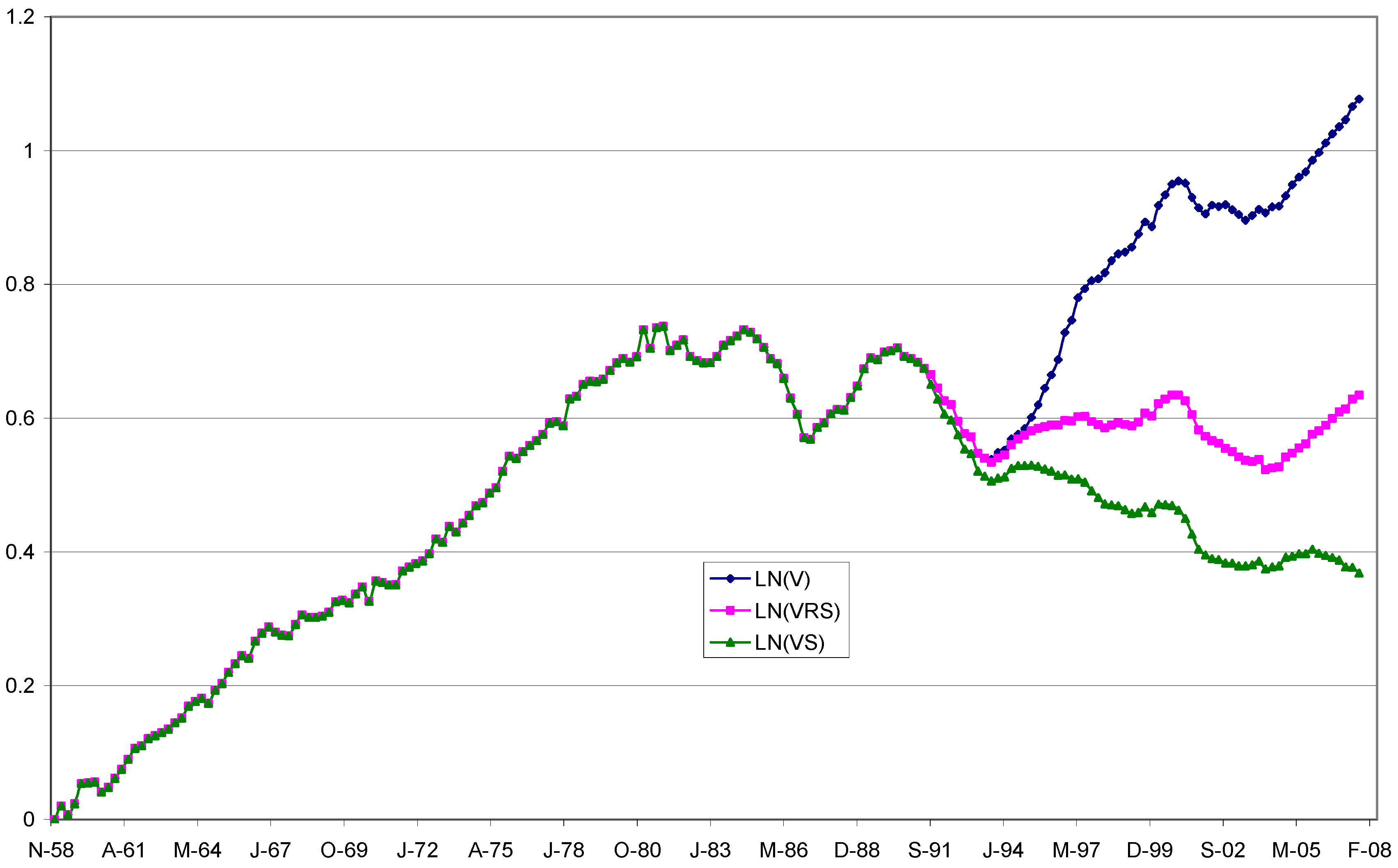
Appendix B. Proof of Proposition 1

To set-up the result, it is first important to recognize that there is a relative opportunity cost to holding money as compared to holding goods for barter. Credit/lending technology is less efficient in a barter economy due to storage and spoilage costs. Given a rate of interest R promised in a monetary economy, if the monetary system suddenly collapses, the expected return in a barter economy becomes (1 + R)(1 − δ) − 1, where 0 δ < 1 is the per-dollar storage and spoilage cost.37 Thus, the relative opportunity cost of holding an amount of money (or goods equivalent to the amount of money) for trade is therefore higher in a monetized economy than in a barter economy by the amount δ(1 + R).
Assuming that the opportunity cost of money is given by the short-term interest rate R t S , the standard optimality condition determining the optimal money holdings m t * is Net Marginal Benefits of Real Money Holdings − R t S = 0. On the other hand, the services that money renders must at least be equal to the transaction services obtained by holding goods for barter, as money is an extension of barter. In other words, money services can be separated into two additive components: (1) the same basic transactional services that goods held for barter provide, plus (2) the reduction of transactional frictions caused by barter.38
The general optimum quantity of money condition above can be re-written by segregating the marginal benefits due to barter and those incremental savings due to instituting a monetized economy at the point of collapse: Net Marginal Benefit of Holding Barter Goods − (1 + R t S )(1 − δ) + 1 + [Net Marginal Benefit of Real Money Holdings − Net Marginal Benefit of Holding Barter Goods] − δ(1 + R t S ) = 0; where the bracketed term corresponds to the marginal cost savings associated with real money holdings relative to barter, i.e., T t m t .
Assume that the institution of money collapses and the economy suddenly reverts back to barter. The quantity of money equation must hold true at the point where the economy transitions into barter.39 People must be indifferent between holding a given amount of real money m t and bartering and thus m t V t B = y t B = C t A + B t ; with V t B 1 representing the velocity of money in that economy. Here, the average real output is the sum of consumption in autarky C t A and the representative basket of goods held for barter B t per-capita, which includes goods purchased by consumers and producers. At the point of collapse, people must be able to purchase the total consumption, which splits into (i) what they can eventually produce and consume in autarky plus (ii) additional goods they are looking to barter for.
I assume that consumption in autarky is related to the amount of goods bartered in the following way C t A = [ V t B 1 ] B t . This condition is an equilibrium resource constraint. Each real unit of money must be ultimately redeemed against its real good (barter) equivalent only once. Of course, the last person left holding the (money) bag loses if money is viewed as worthless. As Ritter (1995) points out, there are two possible ways out of this conundrum. First, the government maintains the convertibility of money into goods/commodities, for example, by raising tax revenues in kind (i.e., non-perishable commodities). The other is that if convertibility is not maintained, the government commits to not using seignorage so that money can be stored away and used again sometimes in the future.
Another reason why money still has value is that autarky production has not started yet, so people do not have the necessary spectrum of goods to barter effectively. For example, State and federal employees, software engineers, and teachers would probably have a hard time bartering the services they produce, and so some economic activities would naturally be impeded. The raison d’être for the velocity V t B being greater than one here is to accommodate this purchase of “autarky” goods before autarky production begins. This latter condition, combined with the quantity equation, implies m t = B t .40
In a pure barter economy, the net marginal benefit of holding one additional unit of real barter goods held as inventory is the value of the incremental goods to be purchased, which are not available in autarky. At the optimum, this value must be equal to the opportunity cost (interest rate net of spoilage due to storage) or (1 + R t S )(1 − δ) 1. The representative basket with B units of barter goods provides a utility of U(B) due to welfare-improving trades. The optimality condition that determines the optimal holdings of barter goods B t * is U ( B t ) B t | B t * = ( 1 + R t S ) ( 1 δ ) 1 . The optimality of the quantity of the unitary basket B t * must be satisfied independently from the monetized economy. Because during the sudden transition to barter, the condition m t = B t holds, the optimal real money balances must also satisfy the same optimality condition with respect to providing equivalent transaction services to those offered by the basket of real barter goods. Because money holdings m t * were optimized before the collapse of the fiat money economy, this leads to m t * = B t * . Hence, the optimum quantity of money m t * can be determined simply by equating the marginal benefits vs. the opportunity cost of holding money in excess of those generated by barter; that is:
T t m t = A × ( 1 λ 4 ) × ( 1 + R t S ) 1 λ 1 × ( 1 + R t L ) λ 1 × y t λ 3 × m t λ 4 = δ ( 1 + R t S )
Rearranging the terms and taking the logs leads to expressing real money balances as (1). From the QTM equation, the real stock of money per-capita is given by m t = y t V t . Using this last equation and taking the logs, the velocity of money can finally be expressed as (2) above. The assumption λ 3 < λ 4 guarantees that the velocity of money rises with real GDP/capita, our index of progress. □

Appendix C. The 2008–2023 Period. A Review of Unconventional Monetary Policies (UMPs) and A Robustness Test of the Long-Run Velocity Relationship
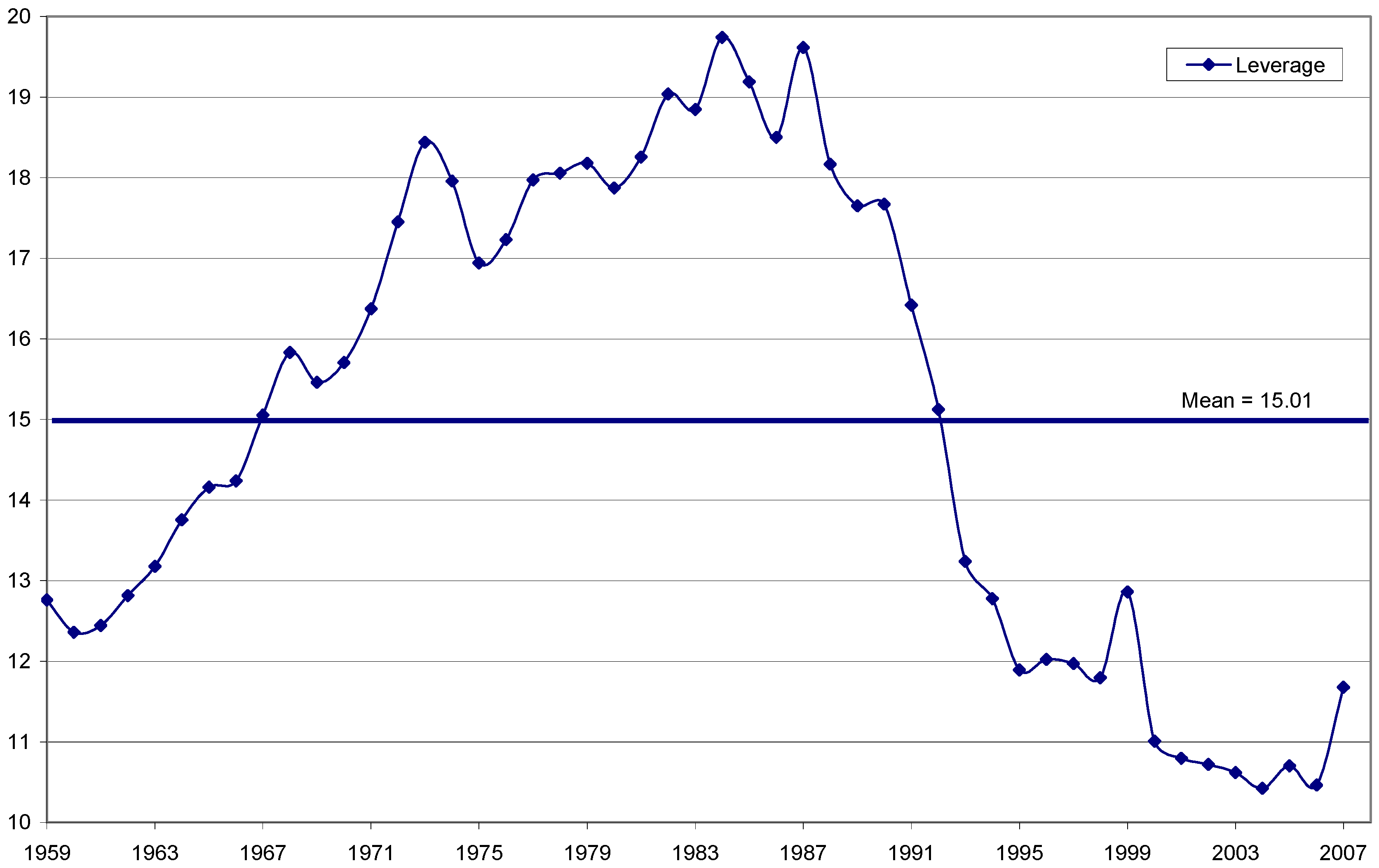
In this appendix, I review the main episodes that constituted a complete shift in U.S. monetary policy away from long-term inflation targeting. These two episodes are: (1) The response to the GFC of 2008 over the period 2008–2014; and (2) the response to the COVID-19 crisis of 2020-present.
Prior to the Great Financial Crisis (GFC) of 2008–2009, monetary policy in most developed economies focused on manipulating a benchmark short-term interest rate. The most popular conceptual reference was the “Taylor rule”, according to which a central bank would adjust its policy rate in accordance with changes in expected underlying inflation and economic growth. Exchange rates, money, and credit aggregates were widely monitored but not targeted directly. In normal times, central banks are neither involved in direct lending to the private sector or the government nor in outright purchases of corporate debt or other types of debt instruments. In the last 15 years, the Federal Reserve (and other central banks) have used monetary policies that are referred to as unconventional monetary policies (UMPs) in response to the 2008 GFC and the 2020 COVID-crisis.
I.
In the aftermath of the 2008 GFC, the U.S. Federal Reserve implemented new monetary policies (UMPs).
(a)
Quantitative Easing (QE): Initially, the US Federal Reserve dropped the target federal funds rate (the borrowing rate between banks) to nearly zero in 2008. As policy rates approached their lower bounds, the conventional implicit guidance of the Taylor rule became and remained inefficient. Trapped at their lowest bound, policy rates lost their power to re-stimulate the economy. As a result, inflation expectations became de-anchored. Threats to price stability were asymmetric and skewed towards a deflationary recession. In that context, the U.S. Federal Reserve initiated Quantitative Easing for the first time in its history in November 2008. That is, it expanded the monetary base (central bank deposits and cash) and purchased government and other securities. QE went beyond straight open market operations as the Federal Reserve balance sheet expanded to acquire assets like high-grade mortgage-backed securities (MBSs), which was a major break with tradition. By March 2009, the Fed had USD 1.75 trillion in bank debt, MBS, and Treasury notes on its balance sheet. In June 2010, the Fed had reached a peak of USD 2.1 trillion in assets. Between 2007 and 2017, the Fed implemented three rounds of QE, and its assets increased from USD 882 billion before the crisis to USD 4.473 trillion—mostly reflecting assets that were not government securities. The Federal Reserve also successfully provided short-term liquidity and collateral to businesses when money market funds failed to do so via the Term Securities Lending Facility and Commercial Paper Finding Facility.
(b)
Forward Guidance (FG): The Fed undertook to provide markets with explicit signals regarding its commitment to maintain policy rates at the lower bound for a significant length of time, thus guiding medium- to long-term interest rate expectations.
Caldara et al. (2020) find that unemployment rose sharply during the GFC and declined steadily thereafter, whereas inflation persistently fell short of the 2% longer-run inflation goal adopted in January 2012. The evidence shows that the QE and FG deployed then eased financial conditions, supported employment, and helped raise inflation toward 2 percent in a manner roughly consistent with expectations at the time. However, PCE inflation ran below 2% for most of the following decade, raising concerns that longer-run inflation expectations could become unanchored or anchored at too low a level. Some survey-based measures of longer-run inflation expectations (such as the Michigan measure) ran below their pre-GFC trend and below levels consistent with the 2% goal. Finally, the QE programs ended in October 2014, but the policy rates remained at their lowest level up until December 2015.
What were the effects on interest rates? In November 2008, the Federal Reserve started buying USD 600 billion in MBSs from commercial banks. This action flooded banks with excess liquidity (cash in their reserve accounts). The excess liquidity had a downward influence on short-term interest rates. After the announcement of the first quantitative easing program, QE-1, the 10-year Treasury yield dropped 107 basis points in two days, demonstrating the short-term implications of quantitative easing. Williams (2014) analyzes the market reaction to the Federal Open Market Committee’s (FOMCs) large-scale asset purchase program (LSAP). He summarizes the evidence, noting that the QE-2 $600 bn of LSAP purchases tended on average to lower the yield on 10-year Treasury bonds by 15–25 basis points. This is roughly the same-sized move in longer-term yields as would be expected from a 0.75–1 percentage point cut in the Federal Funds rate, which was then already at its zero lower bound. Furthermore and independently of the Fed’s policy, it is worth noting that the use of negative (nominal) interest rate policies adopted by major European central banks and the BOJ between 2014 and 2016 tended to reinforce the downward pressure on U.S. interest rates, as it provided no incentive for the Fed to worry about capital outflows from the U.S. to other developed nations.
II.
The 2020 Covid crisis and subsequent inflation acceleration.
(a)
Quantitative Easing during the Covid Crisis of 2020 (QE-4): Overall, the U.S. gross domestic product (GDP) decreased by roughly 2.2% in 2020 due to the Covid pandemic. In reaction to this economic collapse, the Federal Reserve implemented a new round of Quantitative Easing (QE-4). Rates were already low heading into the pandemic, as the Fed funds rate was between 1.5 and 1.75% leading into March 2020. The Fed cut interest rates twice in that month, bringing them to the effective lower bound (0–0.25%). Because rates were already so low, the stimulus to the economy from reducing rates to the lower bound was limited. At the 15 March 2020, meeting, the Fed began QE4, which included monthly purchases of USD80 billion of agency debt and USD40 billion of mortgage-backed securities. As of 15 November 2023, the Fed’s balance sheet amounted to roughly 7.1 trillion U.S. dollars.
(b)
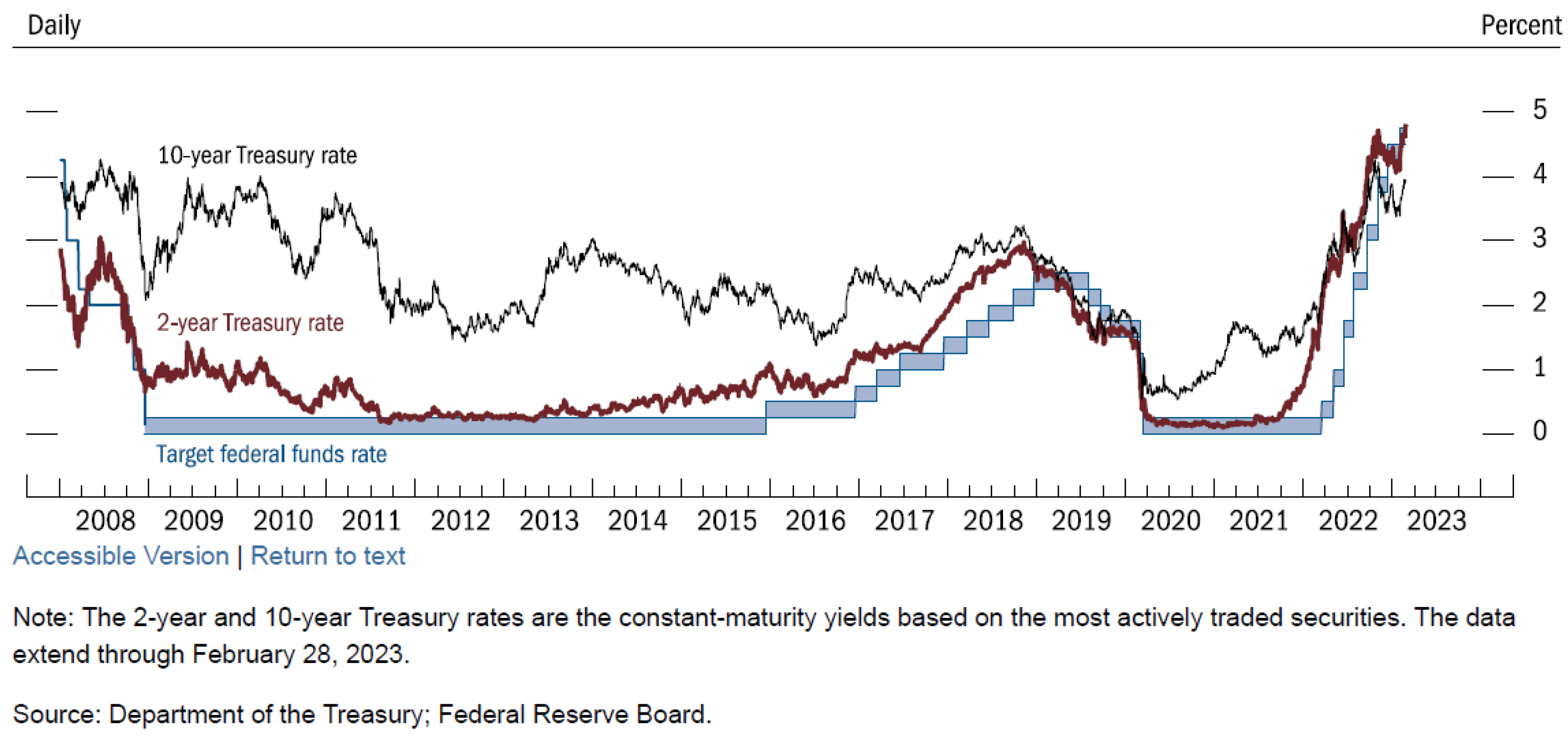
Drastic interest rate policy to combat the resurgence of inflation: In June 2021, inflation in the United States started to rise, with headline PCE at 4.0 percent annually. In the June 2021 FOMC meeting, the committee decided not to raise the policy rate. Although inflation did not slow as expected and, in fact, it rose instead, the FOMC did not increase the policy rate from zero until its March 2022 meeting, at which time headline PCE inflation had risen to more than 6 percent. Subsequently, it raised the federal funds rate at its fastest rate of increase in the history of the federal reserve, going from 0.25% to 4.25% in the span of a year. While this episode falls more under the purview of conventional monetary policy (tightening interest rates in reaction to higher inflation), the wild swing in policy can be seen as unconventional and attributable to an underreaction by the Fed to the economy rebounding faster than expected, which then generated the Fed’s “overraction” with the fast pace raises of the policy rate. Figure A3 below showcases the behavior of key interest rates during these episodes.
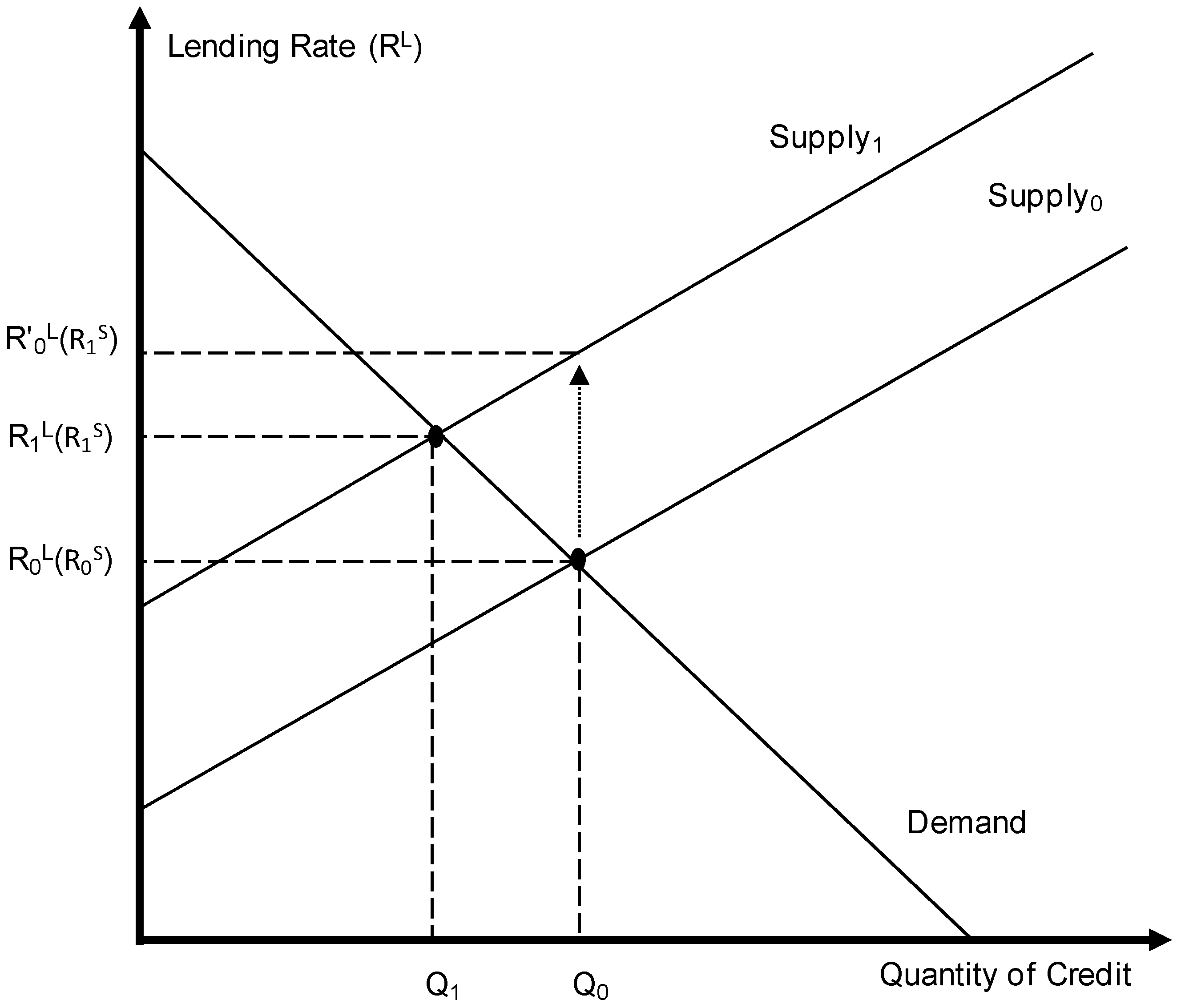
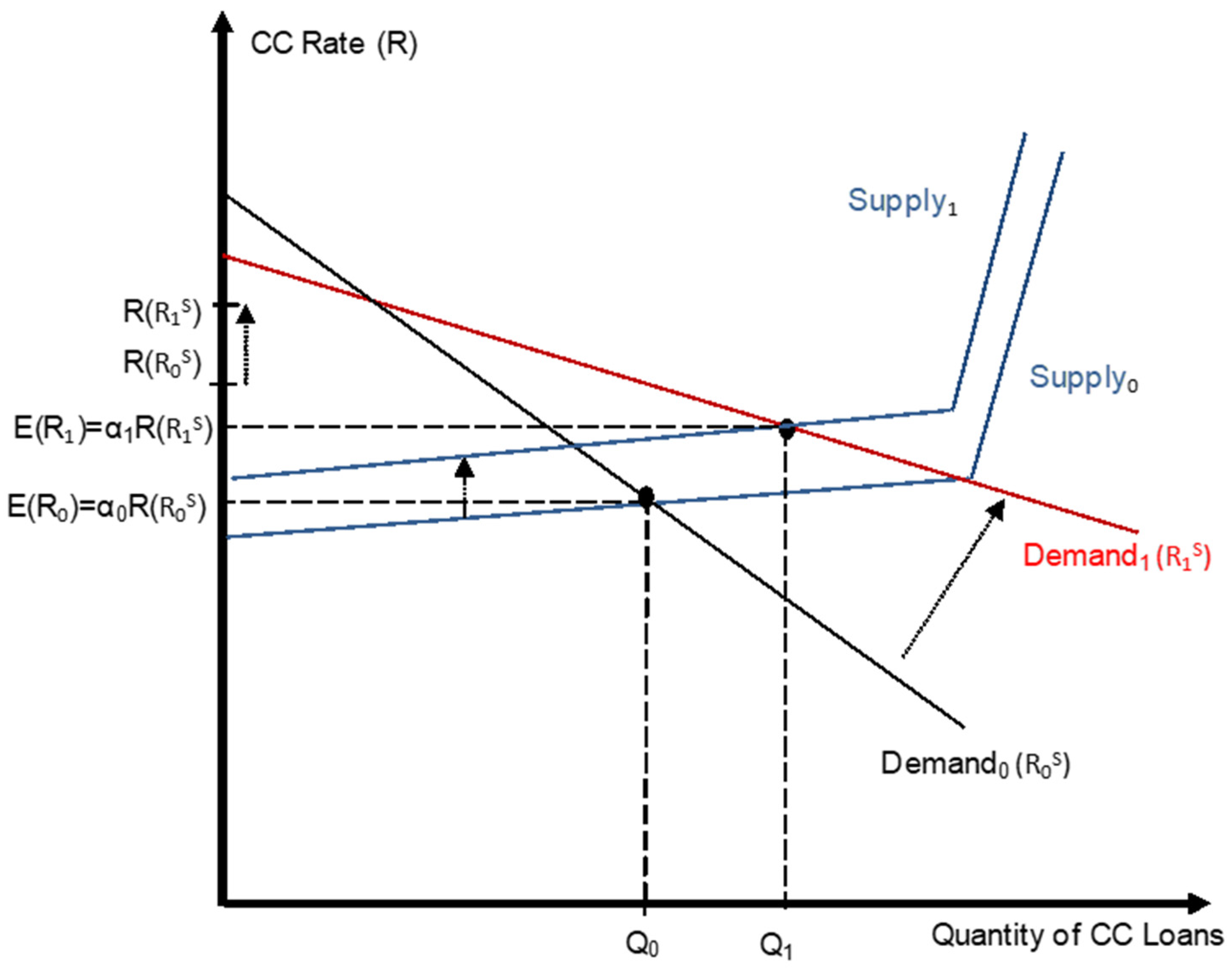
Figure A3. Impact of Fed Policy on Key Interest Rates 2008–2023.
Ijfs 12 00015 g0a3
In conclusion, it is clear that the UMPs adopted during the 2008–2015 and 2020–2023 periods contributed to generating “bigger than normal” shocks to interest rates, relative to the conduct of a Taylor-type adjustment rule that would simply follow the business cycle. It is interesting to note that most of the new money creation that occurred from QE-1 to QE-3 during the GFC did not have an inflationary impact. In fact, the newly created money that was used to finance the large-scale asset purchase programs seemed to have been parked by the banking sector in excess reserves for recapitalization purposes and did not lead to an acceleration in consumption credit (Orlowski 2015; Ennis and Sablik 2019). But at the same time, this policy prevented a dire economic collapse. On the other hand, the spirit of QE-4 during Covid was different, as the new money went directly into the hands of consumers via the U.S. government stimulus package, and eventually, with the economic recovery, this excess money found its way back into the system to generate fast-rising inflation (even though some argue that the trigger was cost-push inflation).
It is also worth noting that the velocity of M1 money appears to fall after the 2008 financial crisis and then levels up after 2016 up until Q1 of 2020 (right before the Covid-crisis). This can be explained by the fact that the U.S. economy suffered a recession during that time (GDP decline and slow growth), while at the same time the unconventional pace of expansionary monetary policy meant that M1 was inflated and this surplus of money (in the form of excess reserves) remained in the system, having a small positive real effect and may have contributed to inflating financial asset prices. Overall, this unconventional policy had an abnormally depressing effect on the velocity of money.
Notwithstanding, the definition of M1 changed after May 2020 to include money market deposits and savings accounts. This distorted the velocity even further, as it makes it look like M1 velocity is dropping precipitously after May 2020 (as there is no harmonization of the old concept with the new one). If we correct for this artificial jump down, we can observe from the data that the velocity is increasing again after Q3 2020 up until 2023 and seems to be rising with real-GDP/capita.
III.
Robustness test of the model for the period 1959–2023
Here I conduct a robustness test of the model extended over the period 1959–2023. The model is slightly modified to account for the change in the definition of M1 after May 2020. To accommodate for this change (as I cannot rebuild the old series due to missing components), I chose to use a dummy d2023 that represents a jump in the series. It also enables us to consider the sudden shift in policy due to Covid. The new equation tested is similar to Equation (3), except for this change.
ln ( V t ) = ln ( α ) + β 1 × R t S + β 2 × R t L + β 3 × ln ( y t ) + β 4 × d 5971 + β 5 × d 2023
I use the same VECM procedure as in the main text.41 The results of the cointegration tests are given in Table A1 below.
Table A1. Robustness Tests: Results for the Log of Velocity of M1 and Adjusted M1 from Jan. 1959–Jul. 2023 on a Quarterly Basis.
The “endogeneized” variable is the Log of money velocity (M1 or AdjustedM1), which following Johansen’s method (1995) has a normalized coefficient of 1. The Adjusted M1 variable is adjusted for the effects of QE-1 to QE-4 (see description in Appendix C). Equations shown are those for whom the trace statistics for the rank of the cointegrating equations reject that the rank is greater than 1 at the 95% level. The Chi2 statistics shows that all parameters in the equations are together significant at least at the 99% level. All coefficients in all the cointegrating equations are significant at least at the 10% level, except the dummy d5971 which is not significant. The High and Low columns represent the 95% confidence interval around the estimate of the coefficient for Ln(realGDPc). The AIC, BIC and HQ criteria in the righmost columns indicate the goodness of fit for the VECM.
LagOptimal Lag
Criterion
Ln VelocityTraceRSRLLnreal GDPcd5971d2023Const.LowHighLn LklhoodChi2AICBICHQ
1None M1 56.924.20−19.781.07−0.021.50−1.511.501.134289160−33.1−33−32.9
2HQIC, SBICM139.962.15−62.370.92−1.00−1.010.24−0.161.99442374−34−33.7−33.3
1None M1 60.826.10−20.401.02−0.03−1.48−1.310.571.474293136−33.1−33−32.8
2 FPE, AIC, HQIC, SBIC M1 45.760.23−58.700.87−0.58−0.980.41−0.141.88442665−34−33.7−33.2
1SBICAdj. M158.731.72−31.551.33−0.24−1.41−2.030.632.03397495−30.7−30.6−30.4
1SBIC Adj. M1 58.714.06−15.571.00−0.18−1.14−1.120.611.393977150−30.7−30.5−30.3
4LR Adj. M1 50.740.72−41.660.94−0.45−1.230.230.171.71406663−30.9−30.1−29
2SBICAdj. M1 ♣♣45.99.25−8.391.00−0.08--−1.500.731.283585218−27.5−27.2−26.8
♣ Means that the VECM includes the seasonal dummy d7982. ♣♣ Means that the VECM includes the seasonal dummies d7982 and d2023.
The velocity of money for the M1 series is extended beyond 2007 by obtaining the series M1V from the FRED website and renormalizing this series to conform to the value of the old velocity as of October 2007. I also constructed an adjusted M1 measure that intends to provide a “correction” for the effects of QE-1 to QE-4. With this new measure, I recomputed the velocity of adjusted money and used this new velocity in the cointegration equation. The tests using this new variable are shown in the last four rows in Table A1.
Let us describe how this Adjusted M1 variable was constructed. Based on the previous discussion regarding the impact of QE on excess bank reserves, I considered that during QE periods, some portion of M1 did not contribute to expanding credit and was just kept by banks as a safe asset. I hypothesize a linear relationship between Ln (excess reserves) and Ln (bank credit). I use the series TOTBKCR (bank credit) and EXCSRESNS (excess reserves) available only after April 1984 in the FRED database. I supplement the Excess Reserves series with the Total Reserves series after October 2020 (since the Excess Reserves series stops then). Using OLS, I estimated the following relationship: Ln(excess reserves) = 4.5 × Ln(bank credit) − 36. The adjusted R-square is 73%. I then estimated the “normal” level of excess reserves with this relationship, which reflects the use of reserves to expand credit. I then computed the variable I call Credit Shortfall = Max [0; (Actual excess reserves − Estimated excess reserves)]. This variable indicates when there is a surplus of M1 that does not contribute to creating credit. I assume that any increases in this surplus from one quarter to the next constitute idle M1, and I subtract it from the actual M1. Thus, Adjusted M1 = M1 − Max [0; Q to Q change in Credit Shortfall]. Overall, the velocity of Adjusted M1 will be greater than M1 velocity in those periods when there is a credit shortfall.
Regarding the findings in Table A1, I confirm that with the inclusion of the dummy d2023 in the model, the best performing cointegration relations for M1 are the ones with lag 2 (with and without the seasonal dummy d7982). In that case, when taking the average for these two equations, I find that the coefficient β 3 = 1 λ 3 λ 4 = 0.895. For the cointegration equations using Adjusted M1, with lags = 1 and 4 being the best fit equations, the average of β 3 = 1.09. That means that given the range of possible values for the long-term real GDP per capita growth rate between 2.12% in 2008 declining to 1.85% in 2023 (from 1959), I find that the estimate for the velocity of money is again given by g V = β 3 × g y , and thus in the first case (with M1) the range for the target inflation rate is [1.66%;1.90%] and in the case of Adjusted M1 it is [2.02%, 2.31%]. The model with Adjusted M1 seems to perform best in terms of predicting a near-2% inflation target, which confirms the analysis conducted in the main text.
Examining the leverage coefficients (for the short-term and long-term interest rates), I find that in the overall best fit model using M1 (Lag = 2), the leverage is estimated to be 62, which is way off compared to the estimate for the banking sector leverage over the period, which is equal to 13.61. Here, we can appreciate the distorting impact of the Fed’s QE policy on interest rates, which leads to a squeeze of long-term interest rates. This distortion makes it appear that to generate these levels of M1 velocity, the banking sector must be dangerously leveraged (from the estimate). However, a more reasonable reading of the leverage coefficient estimates is obtained from the cointegration equation using the Adjusted M1 variable. One case with a good fit (Lag = 1 with seasonal dummy) gives a leverage between 14 and 15.6, which is close to reality but still a bit excessive. Again, this is due to the distorting effect of the Fed’s UMPs during the period. In that case, given the value of coefficient on the Ln (real GDPc), it is worth noting that the type of progress in the transaction technology is estimated to be regime neutral over the period.
Overall, this empirical analysis constitutes a robustness test that is passed with good confirmatory results for the estimates of the long-run inflation target near 2% and depository institutions leverage ratios near their historical average. This is mostly thanks to having developed our adjusted M1 variable, which was purposefully intended to correct for some effects of QE programs on the monetary aggregate.

Notes

1
For instance, in a speech at the St. Louis Fed 28th Annual Policy Conference, Bernanke (2003) introduces the concept of an optimal long-run inflation rate. The speech’s main reference is an article by Coenen et al. (2003), who support a 2% target in order to keep deflation at bay. Clearly, the 2% value has great significance as a threshold point in their model. Nevertheless, no attempt is made in this or other articles in the literature to formally relate the 2% threshold to any underlying macro or microeconomic factors. 2% is indeed a focal point in the literature. Many articles either cite 2% explicitly or give a desired narrow range of around 2%. Summers (1991) asserts that the optimal long-run inflation rate is between 2 and 3%. However, his argument is brief and sketchy and does not justify why this specific range is best. Fischer (1996) lists a series of informal arguments centered on the Phillips curve and the difficulties of dealing with a zero inflation rate for stimulating the economy during slowdown periods. Goodfriend (2002) states that “Evidence from U.S. monetary history suggests that such leeway would be enough to enable a central bank to preempt deflation and stabilize the economy against most adverse shocks”. Only recently, and contrary to the mainstream literature, Blanchard et al. (2010) argue for an inflation target of around 4% in response to the 2008 financial crisis and to deal with liquidity traps.
2
This is not trivial, and the argument requires a separate and extensive analysis of the interaction between the markets for credit card loans and general “bank” loans. Putting these elements together and given that the transactional cost savings of money are reduced when more money-like substitutes (credit cards) are used, I find that there must be a positive relation between transactional cost savings and the financial sector’s net asset returns.
3
The idea has a well-established tradition. Richard Cantillon, John Locke, Knut Wicksell, Irving Fisher, and Milton Friedman all pointed to innovations as a factor speeding-up the velocity of money (Humphrey 1993). Nevertheless, measures of technical progress have not yet been empirically tied to the velocity of money, as conducted here.
4
Due to the non-traditional QE policy measures taken by the U.S. Fed, I intentionally cut my sample before the onset of the 2008 financial crisis to test this model. We also witnessed a revival of unconventional policy measures by the Federal Reserve in the wake of the 2020 covid crisis; thus, that period is not conducive to studying the long-run dynamics of the velocity of money either. Nevertheless, robustness tests are conducted in Appendix C that cover these periods.
5
The same argument is given by Benchimol and Qureshi (2020), who estimate money demand for the US over 1959–2008.
6
In Appendix C, I conduct a discussion of these extraordinary measures and a robustness test of the model for the period 1959–2023 to illustrate how these relationships are impacted. The robustness tests still validate the approach, as the discrepancies in the long-run equilibrium estimates can be explained and reduced using economically grounded arguments and adjustments to M1 that correct for the effects of UMPS.
7
Tobin (1992) is careful to distinguish between the real effects due to the absence of a standard medium of exchange and the use of a numeraire. Of course, changing the units of account (the new numeraire) has no real effect. This is the classical neutrality of money proposition.
8
In this case, I consider that the relevant head count (i.e., per-capita) includes the population of individuals, businesses, and non-federal government entities holding accounts at depository institutions. I thus define the average member of society as a representative domestic economic agent who is a composite of all these categories.
9
I define transaction technology as the medium of exchange (money or barter goods) and the associated devices or methods used to facilitate transactions (for example, credit cards are associated with fiat money).
10
A limitation of this analysis is that since the late 1990s, the source of profits for the banking sector has not been based only on generating a positive net interest margin but also on banking and securitization fees and gains on securities and derivatives.
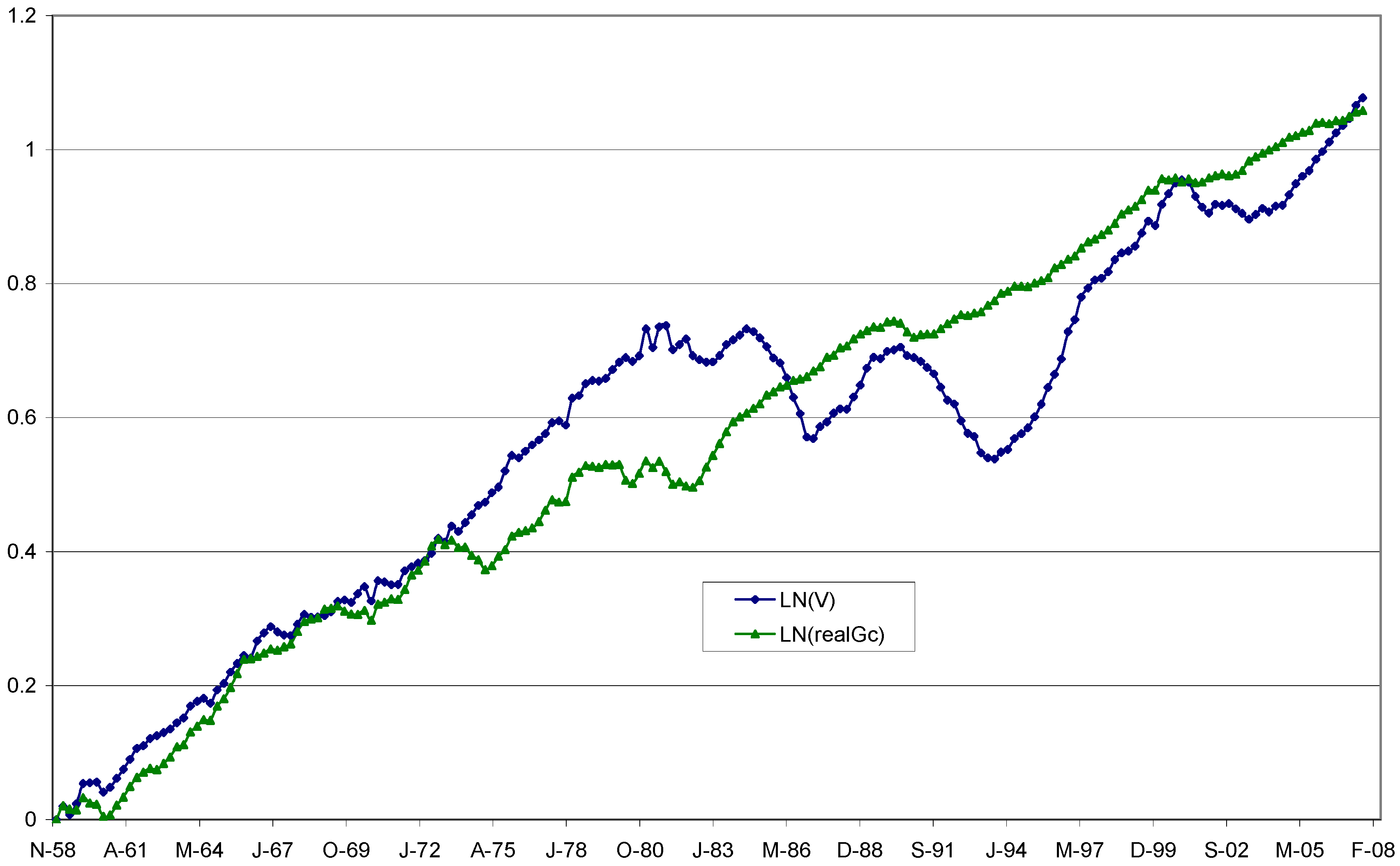
11
I recognize that, strictly speaking, real GDP/capita is not the same as labor productivity measured by output/hour. However, the two are highly correlated. Using FRED quarterly data between 1959 and 2007, the correlation between the two variables is 99.2%, and 98.5% over 1959–2023. Along a steady-state growth path for the economy, it is essentially impossible to separate out the economic effects of real GDP per-capita growth vs. that of labor-augmenting technical progress, as in the long run, these two variables are inextricably tied. This reasoning can be applied to progress in transaction cost savings. My analysis here does not focus on transitional dynamics but on steady-state growth. In that case, the sole engine of economic growth is technical progress.
12
It is possible that more primitive types of money will also receive an efficiency boost. Assuming A > 0 rules out the case where the old type of money leapfrogs the newer type.
13
Note that the cost-saving function must satisfy 0 A t 1 . Using the Quantity Theory of Money equation expressed as M t × V t = Y t , the real stock of money per-capita is given by m t = y t / V t . Thus, the function A t can also be written as A t = A × ( 1 + R t S ) 1 λ 1 × ( 1 + R t L ) λ 2 × V t λ 3 1 × m t λ 3 λ 4 . As long as the velocity of money is not falling to zero and the stock of real money per-capita is not declining, the condition λ 3 < λ 4 plus the proper bound on the constant A are sufficient to ensure that 0 A t 1 . In the limit case where money velocity drops to zero, this constraint can still be met as long as real money per-capita grows faster than the speed of velocity decline.
14
Along Friedman’s line, Wolman (1997) focuses on individual money holdings. He considers the marginal savings in terms of wage earnings due to less time spent transacting. Lucas (2000) also focuses part of his paper on developing a model that incorporates a shopping time constraint, again within a monetized economy.
15
Wolman (1997) assumes satiation in money holdings in order to reproduce Friedman’s (1969) result. Mulligan and Sala-i-Martin (1997) assert that the assumption of satiation can be done away with in their model as long as seignorage falls as the interest rate drops to zero. In other words, the stock of money does not grow faster than the rate of decline of the interest rate. Some cash-in-advance models appear to predict Friedman’s result without resorting to assuming satiation. However, they assume that frictionless barter is achievable as the first-best solution. Recently, a new section of the literature integrates market frictions into hybrid models combining general equilibrium and search models (Aruoba et al. 2007). These models reach conclusions at odds with Friedman’s (1969) recommendation.
16
The sample stopped in 2007 to avoid the noise created by the series of extraordinary short-term measures implemented by the Fed to fight the effects of the 2008 financial crisis. and the reprisal of such measures during the Covid crisis in 2020, followed in 2022 by a complete reversal with fast monetary tightening. In Appendix C, I conduct a robustness test for the period after 2007.
17
The site was no longer supported, and the data were updated as of 2012. The old data can be obtained upon request from the authors.
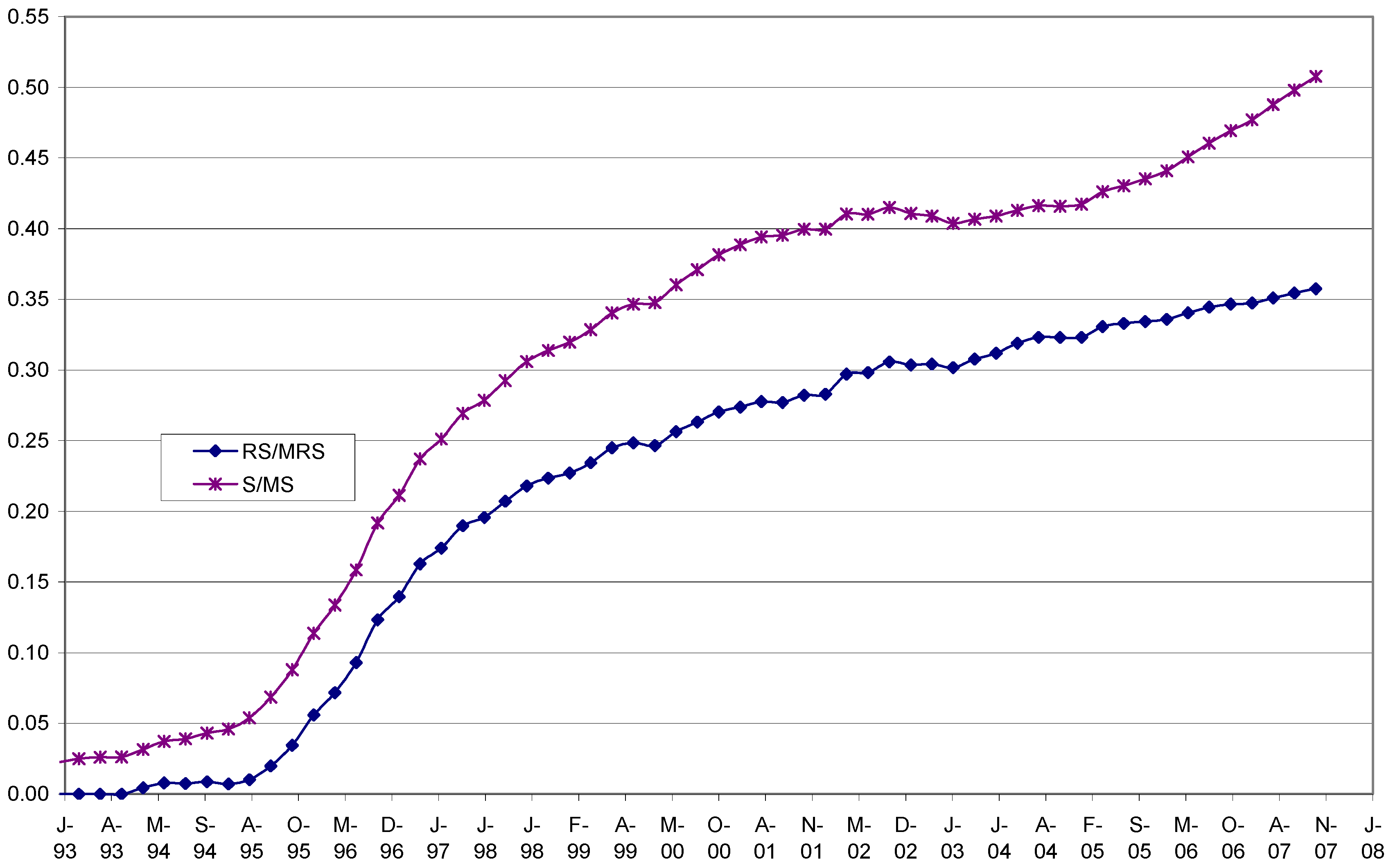
18
Cynamon, Dutkowsky, and Jones’s database tracks commercial demand deposit programs only after 1991. Thus, M1S may have been slightly biased downward prior to 1991.
19
The use of VECM for estimating money demand functions is fairly standard (see, for example, Haug and Tam (2007)). Benchimol and Qureshi (2020) estimate the US money demand on a quarterly basis, as we do here from 1959 until before the onset of the GFC in 2008 and use the VECM framework in their article.
20
I run Augmented Dickey and Fuller (1979) tests with trends for the log of velocity of money (M1, M1RS, and M1S) as well as for SM1 and the log of real GDP per-capita and with drift for the two interest rates. In all cases, the null hypothesis of non-stationarity cannot be rejected at the 1%, 5%, and 10% levels, except for the T-Bill rate, which is rejected at the 5% level but not at the 1% level. The detailed results are obtainable from the author. The other possible issue is the collinearity between the two interest rates used here. However, rather than imposing restrictions, I let the VECM structure speak for itself and determine whether there is an independent cointegrating equation governing the behavior of these two rates, with short-term adjustments away from equilibrium. The empirical results do not support that contention. Any short-term relationship between the two rates will be uncovered by the short-term dynamics of the VECM and thus separated from the cointegrating relationship (3).
21
The definition is different for M1RS and M1S. For M1RS, the variable SM1 only includes retail sweeps. Total sweeps are included in M1S.
22
I excluded instances of rank equal to 2, which occurred mostly when the number of lags equaled 4. These multiple cointegrating equations were economically meaningless. I also ran post-estimation diagnostics on the VECM. Overall, the presented equations were part of VECMs that had stable roots with normally distributed disturbances (except for the short term dynamics of the log of real GDP/capita), and exhibited some residual autocorrelation at all lags up to lag 4. The results are available from the author upon request.
23
I consider that leverage ratios with a value above 100 are outliers and, therefore, are removed from the sample. These are banks and financial institutions with the following NAICS codes: 522110 commercial banks, 522120 savings institutions, 522130 credit unions, and 522190 other depository credit intermediation institutions. After 1999, I added other institutions due to the 1999 banking deregulation. The additional codes are: 522210, 220, 291, 292, 294, 390; 523220; 524126; 127; and 210.
24
I will discuss later why M1 is a better choice to capture the actual leverage parameter.
25
I run VECM “control” experiments without dummy variables, and as can be seen from the bottom half of Table 3, none of the experiments conform to the predictions of the theory, and there is no discernible pattern for any of the money measures.
26
Interestingly, as more lenient reserve requirement rules were enacted since the 1990s, one should have expected leverage to increase in depository institutions, but in fact, one observes the opposite in Figure 3. This might be due to the counteracting effect of the Basel Accords regarding capital adequacy, especially the dip after 1990.
27
Taylor (1998) uses the QTM to informally derive a general Taylor-type rule based on a constant money growth rule. However, he does not specify, nor does he derive a money demand function. Nelson (2008) does present the two rules as antinomic.
28
There is a literature contrasting the effects of either rule in terms of their impact on economic stability (Evans and Honkapohja 2003).
29
A classic article that predicts Friedman’s result is Abel (1987). Mulligan and Sala-i-Martin (1997) provide a great survey in which they find that Friedman’s conclusion is model-dependent. Of course, theoretically, Friedman’s (1969) proposal is subject to the same limitations as mentioned before, given the assumptions of (1) satiation and (2) a pre-existing monetized economy. Also, it should be logically clear that Friedman’s concept is distinct from the issue of a liquidity trap. That is, monetary policy is becoming ineffective to kick-start the economy as the short-term interest is close to zero (Goodfriend 2000; Clouse et al. 2003; Bernanke et al. 2004).
30
While the most recognizable feature of credit cards is their ability to substitute for money, I argue that the key feature of this transmission mechanism is the grace period, which ultimately drives the demand by convenience users and possibly entices credit card users to carry a positive balance due to a lack of vigilance over meeting the card companies’ conditions (Ausubel 1991).
31
Faugere and Van Erlach (2009) find that the Fisher effect on an after-tax basis is indeed present in equity index valuations and Treasury yields.
32
These figures are available from the author upon request.
33
This is assuming the traditional commercial banking model prevails, whereas securitization has changed this situation since the mid-1990s. Currently, about 60% of all credit card loans are securitized (Getter 2008).
34
The higher lending rates (long-term) will put pressure on the long-term bond market, so the yields will go up there too.
35
The analysis is conducted so that the aggregate amount of credit is held constant once the total effects of Figure A1 and Figure A2 are combined. This is a key point because the comparative statics analysis of the transactional cost savings function requires the neat asset return to change, holding M1 constant.
36
It should also be clear to the reader that the above analysis is consistent with the bank “lending channel” approach to monetary policy as developed by Bernanke and Blinder (1988).
37
I assume that spoilage costs affect interest paid and principal in a pure barter economy, so that (1 + R)(1 − δ) − 1 ≥ 0. This is similar to comparing (in the standard macroeconomic growth model) the interest rate in an economy where capital depreciates vs. the case of zero depreciation. With zero depreciation, (1 + R) equals the marginal productivity of capital. With positive depreciation, the new rate is (1 + Rnew) = (1 + R − δ). However, it becomes (1 + Rnew) = (1 + R)(1 − δ). if the interest earned (in goods terms) is subjected to spoilage as well, for example, due to having to store principal and interest before payment.
38
I assume that the marginal benefits of holding barter goods are net of current spoilage costs and that the transaction cost savings from using money are net of the cost of producing money.
39
A case in which money and barter can co-exist for a while is that of hyperinflation. A good reference for a model of the transition from barter to fiat money is Ritter (1995). Ritter’s model is based on Kiyotaki and Wright (1993).
40
My approach implicitly necessitates the presence of a medium of account in the barter economy (a unit basket of goods), which can translate into the real money unit. For example, the medium of account could be a mixture of the reference baskets in the CPI and PPI indexes, and the unit of account is 1 unit of that mixed basket. For a discussion of the difference between medium of exchange vs. medium of account vs. unit of account, see McCallum (2003).
41
We ran the pre-diagnostics for rank and excluded all cointegrating equations with ranks above 2.

References

  1. Abel, Andrew B. 1987. Optimal Monetary Growth. Journal of Monetary Economics 19: 437–50. [Google Scholar] [CrossRef]
  2. Adrian, Tobias, and Hyun Song Shin. 2009. Prices and Quantities in the Monetary Policy Transmission Mechanism. Staff Report No. 396. New York: Federal Reserve Bank of New York. Available online: https://www.econstor.eu/bitstream/10419/60742/1/622777742.pdf (accessed on 6 February 2023).
  3. Anderson, Richard G. 1997. Federal Reserve Board Data on OCD Sweep Account Programs. Available online: http://research.stlouisfed.org/aggreg/swdata.html (accessed on 30 May 2002).
  4. Anderson, Richard G. 2003. Retail Deposit Sweep Programs: Issues for Measurement, Modeling and Analysis. Working Paper 2003-026. St. Louis: Federal Reserve Bank of St. Louis. [Google Scholar]
  5. Aruoba, S. Boragan, Guillaume Rocheteau, and Chirstopher Waller. 2007. Bargaining and the value of money. Journal of Monetary Economics 54: 2636–55. [Google Scholar] [CrossRef]
  6. Ausubel, Lawrence M. 1991. The Failure of Competition in the Credit Card Market. The American Economic Review 81: 50–81. [Google Scholar]
  7. Ausubel, Lawrence M. 1997. Credit Card Defaults, Credit Card Profits, and Bankruptcy. The American Bankruptcy Law Journal 71: 249–70. [Google Scholar]
  8. Baba, Yoshihisa, David F. Hendry, and Ross M. Starr. 1992. The Demand for M1 in the U.S.A., 1960–1988. The Review of Economic Studies 59: 25–61. [Google Scholar] [CrossRef]
  9. Bailey, Martin J. 1956. The welfare cost of inflationary finance. Journal of Political Economy 64: 93–110. [Google Scholar] [CrossRef]
  10. Baumol, William J. 1952. The Transactions Demand for Cash: An Inventory Theoretic Approach. Quarterly Journal of Economics 66: 545–56. [Google Scholar] [CrossRef]
  11. Benchimol, Jonathan, and Irfan Qureshi. 2020. Time-varying money demand and real balance effects. Economic Modelling 87: 197–211. [Google Scholar] [CrossRef]
  12. Bernanke, Ben S. 2003. Remarks by Governor Ben S. Bernanke At the 28th Annual Policy Conference: Inflation Targeting: Prospects and Problems, Federal Reserve Bank of St. Louis, St. Louis, Missouri October 17, 2003. Available online: http://www.federalreserve.gov/Boarddocs/Speeches/2003/20031017/default.htm (accessed on 20 December 2023).
  13. Bernanke, Ben S., and Alan S. Blinder. 1988. Is it Money or Credit, or Both, or Neither? Credit, Money, and Aggregate Demand. American Economic Review 78: 435–39. [Google Scholar]
  14. Bernanke, Ben S., Thomas Laubach, Frederic S. Mishkin, and Adam S. Posen. 1999. Inflation Targeting: Lessons from the International Experience. Princeton: Princeton University Press. [Google Scholar]
  15. Bernanke, Ben S., Vincent R. Reinhart, and Brian Sack. 2004. Monetary Policy at the Zero Bound: An Empirical Assessment. Brookings Papers on Economic Activity 2: 1–78. [Google Scholar] [CrossRef]
  16. Blanchard, Olivier, Giovanni Dell’Ariccia, and Paulo Mauro. 2010. Rethinking Macroeconomic Policy. In IMF Staff Position Note. SPN/10/03. Washington: International Monetary Fund. [Google Scholar]
  17. Bordo, Michael D., and Andrew Filardo. 2005. Deflation in a Historical Perspective. BIS Working Paper No. 186. Basel: Monetary and Economic Department. [Google Scholar]
  18. Brown, Tom, and Lacey Plache. 2006. Paying with Plastic: Maybe Not So Crazy. The University of Chicago Law Review 73: 63–86. [Google Scholar]
  19. Brunner, Karl, and Allan H. Meltzer. 1989. Monetary Economics. Oxford: Basil Blackwell. [Google Scholar]
  20. Caldara, Dario, Etienne Gagnon, Enrique Martinez-Garcia, and Christopher J. Neely. 2020. Monetary Policy and Economic Performance since the Financial Crisis. In Finance and Economics Discussion Series 2020–2065. Washington: Board of Governors of the Federal Reserve System. [Google Scholar] [CrossRef]
  21. Calem, Paul S., and Loretta J. Mester. 1994. Consumer Behavior and the Stickiness of Credit Card Interest Rates. The American Economic Review 85: 1327–36. [Google Scholar]
  22. Carlson, John B., Dennis L. Hoffman, Benjamin D. Keen, and Robert H. Rasche. 2000. Results of a Study of the Stability of Cointegrating Relations Comprised of Broad Monetary Aggregates. Journal of Monetary Economics 46: 345–83. [Google Scholar] [CrossRef]
  23. Clemente, Jesus, Antonio Montañés, and Marcelo Reyes. 1998. Testing for a Unit Root in Variables with a Double Change in the Mean. Economics Letters 59: 175–82. [Google Scholar] [CrossRef]
  24. Clouse, James, Dale Henderson, Orphanides Athanasios, David Small, and Peter L. Tinsley. 2003. Monetary Policy When the Nominal Short-Term Interest rate is Zero. Topics in Macroeconomics 3. [Google Scholar] [CrossRef]
  25. Coenen, Gunter, Athanasios Orphanides, and Volker Wieland. 2003. Price Stability and Monetary Policy Effectiveness When Nominal Interest Rates are Bounded at Zero. Frankfurt am Main: European Central Bank. [Google Scholar]
  26. Dickey, David A., and Wayne A. Fuller. 1979. Distributions of the Estimators for Autoregressive Time Series with a Unit Root. Journal of American Statistical Association 74: 427–81. [Google Scholar]
  27. Dotsey, Michael. 1984. An Investigation of Cash Management Practices and Their Effects on the Demand for Money. FRB Richmond Economic Review 70: 3–12. [Google Scholar]
  28. Dueker, Michael J. 1999. Measuring monetary policy inertia in target Fed funds rate changes. Review, Federal Reserve Bank of St. Louis 81: 3–10. [Google Scholar] [CrossRef]
  29. Dutkowsky, Donald H., and Barry Z. Cynamon. 2003. Sweep Programs: The Fall of M1 and Rebirth of the Medium of Exchange. Journal of Money, Credit and Banking 35: 263–79. [Google Scholar] [CrossRef]
  30. Dutkowsky, Donald H., Barry Z. Cynamon, and Barry E. Jones. 2006. US Narrow Money for the Twenty-First Century. Economic Inquiry 44: 142–52. [Google Scholar] [CrossRef]
  31. Engle, Robert F., and Clive Granger. 1987. Co-integration and Error Correction: Representation, Estimation, and Testing. Econometrica 55: 251–76. [Google Scholar] [CrossRef]
  32. Ennis, Humberto M., and Tim Sablik. 2019. Large Excess Reserves and the Relationship between Money and Prices. Brief 19-02. Richmond: Federal Reserve Bank of Richmond Economic. [Google Scholar]
  33. Evans, George W., and Seppo Honkapohja. 2003. Friedman’s Money Supply Rule vs. Optimal Interest Policy. Working Paper University of Oregon. Oxford: Blackwell Publishing. [Google Scholar]
  34. Faugere, Christophe, and Julian Van Erlach. 2009. A Required Yield Theory of Stock Market Valuation and Treasury Yield Determination. Financial Markets, Institutions and Instruments 18: 27–88. [Google Scholar] [CrossRef]
  35. Fischer, Stanley. 1996. Why Are Central Banks Pursuing Long-Run Price Stability. In Achieving Price Stability. Kansas City: Federal Reserve Bank of Kansas City, pp. 7–34. [Google Scholar]
  36. Friedman, Milton. 1951. Commodity-Reserve Currency. The Journal of Political Economy 59: 203–32. [Google Scholar] [CrossRef]
  37. Friedman, Milton. 1960. A Program for Monetary Stability. New York: Fordham University Press. [Google Scholar]
  38. Friedman, Milton. 1969. The Optimum Quantity of Money and Other Essays. Piscataway: Transaction Publishers. [Google Scholar]
  39. Geanakoplos, John, and Pradeep Dubey. 2010. Credit Cards and Inflation. Games and Economic Behavior 70: 325–353. [Google Scholar] [CrossRef]
  40. Getter, Darryl E. 2008. The Credit Card Market: Recent Trends, Funding Cost Issues, and Repricing Practices; Congressional Research Services Report for Congress. RL34393. Washington, DC. Available online: https://digital.library.unt.edu/ark:/67531/metadc819334/m1/1/ (accessed on 6 February 2023).
  41. Goodfriend, Marvin. 2000. Overcoming the Zero Bound on Interest Rate Policy. Journal of Money, Credit and Banking 32: 1007–35. [Google Scholar] [CrossRef]
  42. Goodfriend, Marvin. 2002. Monetary Policy in the New Neoclassical Synthesis: A Primer. International Finance 90: 165–91. [Google Scholar] [CrossRef]
  43. Greenspan, Alan. 2007. The Age of Turbulence. New York: The Penguin Press. [Google Scholar]
  44. Guerrero, Federico, and Elliott Parker. 2006. Deflation and Recession: Finding the Empirical Link. Economics Letters 93: 12–17. [Google Scholar] [CrossRef]
  45. Haug, Alfred A., and Julie Tam. 2007. A closer look at long-run U.S. Money Demand: Linear or non-linear error-correction with M0, M1 or M2? Economic Inquiry 45: 363–76. [Google Scholar] [CrossRef]
  46. Hetzel, Robert L. 1989. M2 and Monetary Policy. Federal Reserve Bank of Richmond Economic Review 75: 14–29. [Google Scholar]
  47. Hodrick, Robert J., Narayana Kocherlakota, and Deborah Lucas. 1991. The Variability of Velocity in Cash-in-Advance Models. Journal of Political Economy 99: 358–84. [Google Scholar] [CrossRef]
  48. Humphrey, Thomas M. 1993. The Origins of Velocity Functions. Federal Reserve Bank of Richmond Economic Quarterly 79: 1–17. [Google Scholar]
  49. Ireland, Peter N. 1994. Money and Growth: An Alternative Approach. The American Economic Review 84: 47–65. [Google Scholar]
  50. Ireland, Peter N. 1995. Endogenous Financial Innovation and the Demand for Money. Journal of Money, Credit and Banking 27: 107–23. [Google Scholar] [CrossRef]
  51. Ireland, Peter N. 2008. On the Welfare Cost of Inflation and the Recent Behavior of Money Demand. American Economic Review 99: 1040–52. [Google Scholar] [CrossRef]
  52. Jafarey, Saqib, and Adrian Masters. 2003. Output, Prices, and the Velocity of Money in Search Equilibrium. Journal of Money, Credit and Banking 35: 871–88. [Google Scholar] [CrossRef]
  53. Johansen, Soren. 1988. Statistical Analysis of Cointegration Vectors. Journal of Economic Dynamics and Control 12: 231–54. [Google Scholar] [CrossRef]
  54. Johansen, Soren. 1991. Estimation and Hypothesis Testing of Cointegration Vectors in Gaussian Vector Autoregressive Models. Econometrica 59: 1551–80. [Google Scholar] [CrossRef]
  55. Johansen, Soren. 1995. Likelihood Based Inference in Cointegrated Vector Autoregressive Models. Oxford: Oxford University Press. [Google Scholar]
  56. King, Robert G., Charles I. Plosser, James H. Stock, and Mark W. Watson. 1991. Stochastic Trends and Economic Fluctuations. American Economic Review 81: 819–40. [Google Scholar]
  57. Kiyotaki, Nobuhiro, and Randall Wright. 1993. A Search-Theoretic Approach to Monetary Economics. American Economic Review 83: 63–77. [Google Scholar]
  58. Lucas, Robert E., Jr. 1994. On the Welfare Cost of Inflation. Center for Economic Policy Research, Stanford University. February. Available online: https://books.google.fr/books/about/On_the_welfare_cost_of_inflation.html?id=xSrYzwEACAAJ&redir_esc=y (accessed on 6 February 2023).
  59. Lucas, Robert E., Jr. 2000. Inflation and Welfare. Econometrica 68: 247–74. [Google Scholar] [CrossRef]
  60. Marty, Alvin L. 1999. The Welfare Cost of Inflation: A Critique of Bailey and Lucas. St. Louis: Federal Reserve Bank of St. Louis, pp. 41–46. [Google Scholar]
  61. McCallum, Bennett T. 2003. Monetary Policy in Economies with Little or No Money. Pacific Economic Review 9: 81–92. [Google Scholar] [CrossRef]
  62. Miyao, Ryuzo. 1996. Does a Cointegrating M2 Demand Relation Really Exist in the United States? Journal of Money, Credit, and Banking 28: 365–80. [Google Scholar] [CrossRef]
  63. Mulligan, Casey B., and Xavier X. Sala-i-Martin. 1996. Adoption of Financial Technologies: Implications for Money Demand and Monetary. NBER Working Paper 5504. Cambridge: National Bureau of Economic Research. [Google Scholar]
  64. Mulligan, Casey B., and Xavier X. Sala-i-Martin. 1997. The Optimum Quantity of Money: Theory and Evidence. Journal of Money, Credit and Banking 29: 687–715. [Google Scholar] [CrossRef]
  65. Nelson, Edward. 2008. Friedman and Taylor on Monetary Policy Rules: A Comparison. Federal Reserve Bank of St. Louis Review 90: 95–116. [Google Scholar] [CrossRef]
  66. Norman, Ben, Rachel Shaw, and George Speight. 2006. The History of Interbank Settlement Arrangements: Exploring Central Banks’ Role in the Payment System. London: Bank of England. [Google Scholar]
  67. Orlowski, Lucjan T. 2015. Monetary expansion and bank credit: A lack of spark. Journal of Policy Modeling 37: 510–20. [Google Scholar] [CrossRef]
  68. Orphanides, Athanasios. 2007. Taylor Rules. Washington: Board of Governors of the Federal Reserve System. [Google Scholar]
  69. Park, Albert. 2006. Risk and Household Grain Management in Developing Countries. The Economic Journal 116: 1088–15. [Google Scholar] [CrossRef]
  70. Poole, William. 2006. The Fed’s Monetary Policy Rule. Federal Reserve Bank of St. Louis Review 88: 1–11. [Google Scholar] [CrossRef]
  71. Reynard, Samuel. 2006. Money and the Great Disinflation. Swiss National Bank Working Paper 2006–2007. Bern and Zurich: Swiss National Bank. [Google Scholar]
  72. Ritter, Joseph A. 1995. The Transition from Barter to Fiat Money. The American Economic Review 85: 134–149. [Google Scholar]
  73. Sriram, Subramanian S. 1999. Survey of Literature on Demand for Money: Theoretical and Empirical Work with Special Reference to Error-Correction Models. IMF Working Papers. Washington: International Monetary Fund. [Google Scholar] [CrossRef]
  74. Stavins, Joanna. 1996. Can Demand Elasticities Explain Sticky Credit Card Rate? New England Economic Review (July/August). Boston: Federal Reserve Bank of Boston. [Google Scholar]
  75. Summers, Lawrence. 1991. Price Stability: How Should Long-Term Monetary Policy Be Determined? Journal of Money, Credit and Banking 23: 625–31. [Google Scholar] [CrossRef]
  76. Taylor, John B. 1993. Discretion versus Policy Rules in Practice. Carnegie-Rochester Conference Series on Public Policy 39: 195–214. [Google Scholar] [CrossRef]
  77. Taylor, John B. 1998. An Historical Analysis of Monetary Policy Rules. NBER Working Paper 6768. Chicago: University of Chicago Press. [Google Scholar]
  78. Tobin, James. 1956. The Interest Elasticity of Transactions Demand for Cash. Review of Economics and Statistics 38: 241–47. [Google Scholar] [CrossRef]
  79. Tobin, James. 1992. Money—For New Palgrave Money and Finance. Cowles Foundation Discussion Paper 1013. London: Palgrave Macmillan. [Google Scholar]
  80. Wicksell, Knut. 1936. Interest and Prices. Translation of 1898 edition by R. F. Kahn. London: Macmillan. [Google Scholar]
  81. Williams, John C. 2014. Monetary Policy at the Zero Lower Bound: Putting Theory into Practice. Washington: Hutchins Center on Fiscal & Monetary Policy at Brookings. [Google Scholar]
  82. Wolman, Alexander L. 1997. Zero Inflation and the Friedman Rule: A Welfare Comparison. Federal Reserve Bank of Richmond Economic Quarterly 83: 1–21. [Google Scholar]
Figure 1. Indexed Log of Narrow Money Velocity (M1, M1R1, M1S) 1959–2007.
Ijfs 12 00015 g001
Figure 2. Indexed Log of M1 Velocity vs. Log Real GDP/capita 1959–2007.
Ijfs 12 00015 g002
Figure 3. Asset/Equity (leverage) for Depository Institutions. 1956–2007. Source: Compustat. Outlier values above 100 removed.
Ijfs 12 00015 g003
Figure 4. Retail and total sweeps, respectively, as % of M1RS and M1S 1994–2007.
Ijfs 12 00015 g004
Table 1. Inflation Targeting by G-7 Central Banks. Source: Reserve Bank of New Zealand.
CountryDate AdoptedTargetTarget Variable
Australia1993Average of 2–3% over the medium termUnderlying PI up until October 1998 CPI thereafter
CanadaFebruary 1991Midpoint 2% + 1% bandCPI
FinlandFebruary 19932% no explicit bandCPI excluding indirect taxes, subsidies and housing-related costs
New ZealandApril 19880–3%CPI excluding interest
SpainNovember 19942%CPI
SwedenJanuary 1993Midpoint 2% + 1% bandCPI
U.K.October 19922.5% + 1% reporting rangeRetail price index excluding mortgage interest payments
U.S.January 20122%CPI and/or PCE
Table 2. Innovations Applicable to Transaction Technologies.
Transaction TechnologySample PeriodFed ChairmanshipInnovations Affecting Money Supply and Transaction TechnologyType of Progress
CM1959–71Mc Chesney-Martin 51–70Visa and American Express Cards (1958)New Biased
First fully transistorized IBM 7090 mainframe computer (1959)Neutral
GE’s ERMA Computer to Process Checks (1959)New Biased
General purpose credit cards (BofA) (1966)New Biased
ATMs (1967)New Biased
Information Management System (IBM, 1968)Neutral
Magnetic Swipe Cards (1969)New Biased
Microprocessor (1970)Neutral
Heap Leach Technology for Gold Mining (1970)Old Biased
Clearing House Interbank Payment System (CHIPS, 1970)New Biased
FM1972–82 Automated Clearing House (ACH, 1972)New Biased
First PC Altair (1975)Neutral
Burns 70–78Telephone Banking (1979)New Biased
Miller 78–79Software Standardization of Fedwire System (1980)Neutral
Volcker 79–87Activated Carbon Processes in Gold Mining (1980)Old biased
NOW Accounts (1981), Super NOWs and MMDAs (1982)---
Commodore 64 (1982)Neutral
Lotus 123 (1982)Old Biased
1983–93Volcker 79–87
Greenspan 87–06
Graphic User Interface (1983)Neutral
Windows 1.0 (1985)Neutral
386 chip (1985)Neutral
PC-Based Banking Clearinghouse Item Processing System (1986)Neutral
World Wide Web (1989)Neutral
Consolidation of Mainframe Computers at Fedwire (1990)New Biased
Pentium Chip (1993)Neutral
1994–07 Web Browser Mosaic and Netscape (1994)Neutral
Greenspan 87–06“All Electronic” Banking Clearinghouse ACH (1994)Neutral
Windows 95 (1995)Neutral
Bernanke 06–14Online Banking (1995)New Biased
Completion of High-Speed Network FEDNET (1996)Neutral
TBD Beyond 2007Bernanke 06–14
Yellen 14–18
Powell 18–
Digital MoneyNew Biased
E-barterOld Biased
Table 3. Cointegration Results for the Log of Velocity of M1, M1RS and M1S from Jan. 1959–Oct. 2007 on a Quarterly Basis.
The “endogeneized” variable is the Log of money velocity (M1, M1RS or M1S), which following Johansen’s method (1995) has a normalized coefficient of 1. All samples start on January 1959 and end October 2007. All trace statistics for the rank of the cointegrating equations reject that the rank is greater than 1 at the 95% level and thus point to a unique cointegrating relation in each row. The Chi2 statistics shows that all parameters in the equations are together significant at least at the 99% level. Unless noted, each coefficient in all the cointegrating equations is significant at least at the 99% level. The High and Low columns represent the 95% confidence interval around the estimate of the coefficient for Ln(realGDPc). The AIC, BIC and HQ criteria in the righmost columns indicate the goodness of fit for the VECM. The bottom of the table shows results when dummy variables are excluded.
LagOptimal Lag CriterionLn VelocityTraceRSRLLn Real GDPcd5971SM1ConstLowHighLn LklhoodChi2AICBICHQ
1SBIC M1 22.416.10−15.500.95−0.14---−1.030.761.132998448−30.6−30.5−30.4
2HQICM12114.91−15.090.85−0.21---−0.940.641.073030265−30.8−30.6−30.2
4LR, FPE, AIC M1 30.215.42−16.920.81−0.3---−0.540.611.003049326−30.8−30.2 −29.3
1HQIC, SBIC M1 21.315.21−15.010.93−0.14---−0.920.751.113001425−30.6−30.4−30.3
4LR, FPE, AIC M1 27.814.05−15.80.80−0.29---−0.480.620.993053349−30.8−30.2−29.2
2HQIC M1RS 57.97.37−5.060.58−0.15−0.29−0.220.420.743810563−38.7−38.4 −37.8
4LR, FPE, AIC M1RS 54.212.64−13.190.84−0.23−0.69−0.790.581.113858267−38.9−38 −36.8
2HQIC M1RS 62.97.00−4.890.59−0.15−0.3−0.230.420.753814485−38.7−38.3−37.7
4LR, FPE, AIC M1RS 60.711.43−12.820.91−0.22−0.78−0.980.641.193864244−38.9−38 −36.7
2HQIC, SBICM1S56.17.93−5.400.64−0.13−0.35−0.460.470.813765553−38.3−37.9−37.4
3FPE, AICM1S53.68.29−6.420.6−0.18−0.39−0.250.420.783794497−38.4−37.8−36.9
4LRM1S55.213.70−13.90.89−0.21−0.58−0.990.611.163808275.4−38.4−37.5−36.2
2HQIC M1S 60.47.62−4.920.62−0.13−0.33−0.390.450.783769470−38.2−37.8−37.2
4LR, FPE, AICM1S 59.813.00−13.410.88−0.21−0.58−0.920.611.153812239−38.3−37.4−36.1
1SBICM1 12.717.18−15.471.12------−1.720.991.242757200.7−28.2−28.1 −28
2HQICM1 11.916.42−14.941.10------−1.80.941.252783201−28.4−28.2 −28
4LR, FPE, AICM1 20.119.41−18.211.20------−2.231.011.382792177−28.5−28 −27.5
1SBICM1RS 27.611.18−5.730.49------−0.110.410.582776335.1−28.4−28.3 −28.2
2HQICM1RS 25.522.33−17.280.57------−0.330.320.83280059.9−28.6−28.4 −28.1
4LR, FPE, AICM1RS 24.7−10.6315.940.33------0.380.180.492816110−28.7−28.3−27.7
4LR, FPE, AICM1S29.2−9.5716.130.09------1.02−0.050.242812114−28.7−28.3−27.7
♣ Means that the VECM includes the seasonal dummy d7982.
Disclaimer/Publisher’s Note: The statements, opinions and data contained in all publications are solely those of the individual author(s) and contributor(s) and not of MDPI and/or the editor(s). MDPI and/or the editor(s) disclaim responsibility for any injury to people or property resulting from any ideas, methods, instructions or products referred to in the content.

