1. Introduction
Portfolio optimization is regarded as an attractive topic for most researchers. Its major highlight consists of determining the assets’ optimal weight by increasing its expected returns and also by minimizing risk. The initial portfolio theory, which provides the solution to the trade-off between minimizing risk and maximizing expected returns, was given by
Markowitz (
1952) based on Mean Variance (MV). The MV model is generated based on a set of constrained assumptions such as the normal distribution of stock market returns, making it difficult to use this model for a practical stock market. Since
Markowitz (
1952) developed the Modern Portfolio Theory (MPT), the portfolio optimization literature review has made substantial progress. Several portfolio optimization methods have been used; among them,
Sharpe (
1963) was the first to attempt to simplify the Markowitz model by developing a particular model based on the simplification of the variance–covariance matrix in order to reduce the computational burden and proposed a diagonalization of this matrix based on the single-index model.
Sharpe (
1964) developed the market model by assuming a linear relationship between a stock’s return and the overall market return. It is based on the assumption that investors are risk-averse and will only invest in an asset if it offers a higher expected return than a risk-free asset. Then, following his work concerning the applicability of the variance–covariance matrix,
Sharpe (
1971) developed a new model called the Capital Asset Pricing Model (CAPM) which consists of measuring the degree of sensitivity of the return of an asset to that of the market.
Markowitz (
1981) developed a multi-index model, which is a generalization of Sharp’s single index model into a multi-index model offering investors the possibility of investing in an international market with several stock market indices. The Black–Litterman model developed by
Black and Litterman (
1990) is an extension of mean-variance optimization that allows investors to incorporate their own views about the expected returns of different assets into the portfolio optimization process.
Lai (
1991) proposed a multiple-objective approach, showing that the preference of the investor can be incorporated in a programming problem of polynomial purpose from which a portfolio selection with skewness is determined to improve the optimization quality.
Konno and Yamazaki (
1991) presented that risk function can deal with most of the difficulties associated with the traditional Markowitz’s model while preserving its advantages over equilibrium models. In order to improve the
Konno and Yamazaki (
1991) model,
Speranza (
1993) proposed a linear combination between the absolute deviation below the mean and the absolute deviation above the mean as a measure of risk. When the used data represent an asymmetry of information, the variance and the absolute deviation measures are symmetrical and do not allow for the asymmetry of the data. To solve this problem,
Hamza and Janssen (
1995) proposed a convex combination of the two semi-variances of the portfolio return compared to its expected return as a measure of risk.
Young (
1998) proposed a criterion called “minimax” to measure the risk in order to optimize an equity portfolio. The portfolio is chosen that minimizes the maximum loss over all past observation periods, for a given level of return.
Ryoo (
2007) used the Mean Absolute Deviation (MVD) model as a replacement for the MV model, knowing that it implies absolute variance as a risk factor for calculating the large-scale optimization problems corresponding to the portfolio. An improved portfolio optimization model ensures an efficient frontier which enables investors to obtain better expected returns at the lowest level of risk (
Lai et al. 2018). Moreover, a highly efficient portfolio optimization model is required to evolve in the investment management areas (
Bielstein and Hanauer 2019).
Antony (
2020) provides a detailed overview of the intersection between behavioral finance and portfolio management. The article highlights the limitations of traditional finance theories and the emergence of behavioral finance as an alternative approach. It identifies various behavioral biases that can impact investment decision-making and discusses effective portfolio management strategies that can address these biases. The article also examines the implications of behavioral finance for institutional portfolio management and the role of policymakers in promoting effective portfolio management. Overall, the article provides important insights into the relevance of behavioral finance to portfolio management.
Dospinescu and Dospinescu (
2019) proposed a profitability regression model that is applicable to the financial communication of the Romanian stock exchange’s companies. The authors collected and analyzed data from 56 listed companies in Romania to test the model’s efficacy, and the study concluded that the model is capable of identifying the factors that influence company profitability and predicting future profitability. The authors recommend using the model to improve financial communication strategies for companies and to make informed investment decisions for investors. The article provides valuable insights into the financial communication practices of Romanian companies and offers a significant contribution to the literature on financial communication and investment analysis.
Eckert and Hüsig (
2021) presents a thorough analysis of innovation portfolio management with a focus on digital service innovations. The article delves into the challenges that organizations face while managing their portfolios of digital service innovations, including the difficulty of balancing short-term and long-term investments, managing diverse innovation projects, and assessing and managing risks. The authors explore several approaches to innovation portfolio management, including resource-based, market-based, and balanced approaches. They recommend future research areas such as the need for more empirical studies of innovation portfolio management practices, the development of new theoretical frameworks, and the use of new data sources and tools for informed decision-making. Overall, the article offers a comprehensive overview of the challenges and opportunities in managing portfolios of digital service innovations. In addition,
Liu et al. (
2022) investigates the impact of risk forecast and risk tolerance on portfolio management through a case study of the Chinese financial sector. The authors use a two-stage modeling approach that involves estimating the risk forecast with GARCH models and assessing the risk tolerance of different investors with stochastic dominance analysis. The study shows that risk forecast and risk tolerance play a crucial role in portfolio management decisions and that investors’ risk tolerance can be influenced by socioeconomic and demographic factors. The authors suggest recommendations for investors and policymakers to effectively manage risk in their investment portfolios. The article contributes to the existing literature on risk management and portfolio optimization.
Saleem et al. (
2023) examines the performance of three different asset classes—FAANG stocks, gold, and Islamic equity—during the COVID-19 pandemic and their implications for portfolio management. The study finds that FAANG stocks, which refer to the five most prominent U.S. technology companies—Facebook, Amazon, Apple, Netflix, and Google—have significantly outperformed the other two asset classes during the pandemic. The article discusses how this may be due to the increased reliance on technology and e-commerce during the pandemic, which has benefited these companies. Overall, the article suggests that the performance of these asset classes during the pandemic has significant implications for portfolio management, and investors should consider the risks and opportunities associated with each asset class before making investment decisions.
Topological Network Structures (TNS) are one of the most used techniques to prove their performance in different domains. TNS is significant and fundamental; several researchers used this technique with broad applications in multiple domains, such as characterizing the behaviors of proteins in biological systems (
Farkas et al. 2011), and the controllability of transport and engineered systems (
Mangan 2003;
Verma et al. 2016).
Suvilehto et al. (
2015) made a dynamic process description in social systems.
Burt et al. (
2000) used a network structure of social capital to examine arguments and evidence about the relationship between social media and social capital.
Network Theory has been applied in analyzing the stock market’s topology, in particular, portfolio optimization by different methods and approaches.
Li et al. (
2019) used network topology for portfolio optimization, regarding the complicated financial network as a typical example to display the dependence of the network topology on its function.
Clemente et al. (
2021) explained the Network Structure role on financial markets for improving the portfolio selection process, then formulated and solved the asset allocation problem.
Ma et al. (
2021) used deep learning and machine learning based on historical data stocks of China Securities 100 index, covering the period from 2007 to 2015, for return prediction; this article provides investors with guidance on constructing a model that predicts daily trading investment returns using a multivariate forecast and a random forest approach.
Yan et al. (
2022) introduced the P/E Ratio Network analysis as an alternative to the MV analysis for portfolio optimization, and finds that the size of the portfolio optimized by the P/E Ratio Network has increased significantly to mitigate systemic risk, while MV portfolios were insufficiently diversified. In Network Theory, centrality measures highlight the relative importance of nodes in a network, which are the most fundamental used measures to reveal the structure of the network (
Zhu et al. 2021;
Hu et al. 2020). Using these measures, investment decisions are typically made by choosing central or non-central network assets. The strategy of non-central investment affirms that a portfolio comprising the peripheries of the network has a greater potential for diversification and thus is exposed to minimum risk (
Peralta and Zareei 2016;
Pozzi et al. 2013;
Onnela et al. 2003).
According to numerous research, topological structures of networks through hierarchical clustering methods can be used to reveal the cross-correlations across different assets (
Markowitz 1952;
Tumminello et al. 2005). For instance, the MST has been used to investigate the correlation structure of individual stocks.
Onnela et al. (
2003) demonstrated that on the network’s outer sheets generated by the MST method are always located the nodes of the minimum risk portfolio. In this respect, further research highlights how the affectation of the constructed portfolio’s performance can be caused due to the topological positions of the stocks (
Pozzi et al. 2013).
Nanda and Tiwari (
2010) demonstrates that the Network Topology ciphers the complex dependency structure of financial equities with an extraction of the hierarchical and grouping properties, and decreases the complexity of the data while maintaining the fundamental characteristics of the information. Most empirical studies have used the MST as the backbone for their financial networks, because the complex networks’ functionality depends on their underlying structure as well as structural stability (
Plerou et al. 2002).
In the field of portfolio optimization, previous studies have mainly focused on traditional methods such as Markowitz’s mean-variance optimization, CAPM, and APT. However, these methods have limitations such as sensitivity to input parameters and estimation errors, and they assume normality in returns. Researchers have proposed alternative methods such as the Minimum Spanning Tree (MST) approach. The MST approach is a network-based method that uses the MST tree algorithm to identify key relationships among assets in a portfolio. This approach has been found to be effective in minimizing risk, diversifying portfolios, and reducing the number of assets. This proposal aims to fill a research gap by investigating the use of the MST method in portfolio optimization, specifically in portfolio optimization and comparison tasks. Previous studies have explored the effectiveness of the MST method in portfolio optimization, but this proposal seeks to use it for portfolio comparison with traditional methods to prove its performance and identify effective portfolio construction strategies. This research gap addresses the need for more reliable and robust portfolio optimization techniques that can adapt to changing market conditions and support informed investment decisions.
Several studies on the MST algorithm attest to it having very high average performance. To implement this method, for asset selection and capital allocation, a portfolio objective is set, derived from the return information of the listed companies belonging to the MASI index, by constructing a Network Structure using the MST method to form connections among stocks by defining a node for each selected stock in the network. One must identify potential connections in the network using the Gower distance metric as a similarity measure. From the constructed Network Structure, the DC has been used for portfolio selection and the weighted degrees are derived for the capital allocation stage using IDCP. Finally, two suggested portfolios are created: the MST-Portfolio using 63 stocks for portfolio selection and IDCP for portfolio allocation, and the MST-Portfolio 2 using 32 stocks extracted based on the DC measure for the portfolio selection stage and IDCP for portfolio allocation. These portfolios are compared with the EW Portfolio, MV Portfolio, and according to the backtesting result, to determine the well-performed and robust portfolios.
The aim of the study is to explore the efficacy of utilizing the MST method in both portfolio optimization and portfolio comparison tasks. The objective is to offer a fresh and innovative approach to assess portfolio performance and to identify the most efficient strategies for constructing portfolios. This paper investigates how effective the MST method is in portfolio optimization and portfolio comparison tasks compared to traditional methods such as MV Portfolio and EWP.
The paper is structured as follows:
Section 2 presents a data description and methodology,
Section 3 presents the results, the materials and methods used are discussed in
Section 4, and
Section 5 presents the discussions. Finally,
Section 6 concludes the paper.
2. Data & Methodology
2.1. Data
We collected daily historical log returns based on stock price data composing the MASI index in the Moroccan Stock Exchange (MSE) market, spanning the time frame from 2 January 2013 to 27 October 2022. The used data includes 63 stocks, for which the data are available, since there were other companies that entered the Casablanca Stock Exchange (CSE) market during this period, represented by missing data, and, for this reason, they were removed.
The used data are composed of essentially close historical prices converted into daily historical log returns. Thus, every single stock from the analyzed data is represented by a daily return vector. The data set contains the stocks represented as follows: Attijariwafa Bank (AWB), Itissalat Al-Maghrib (IAM), Microdata (MIC), Banque Centrale Populaire (BCP); the others have corresponding symbols: AFI, AFG, AGMA, ALC, ALM, ATS, AUH, AUN, BMA, BOA, BMCI, CAS, CDM, CIH, CIM, CRD, CSM, CTM, DRC, DLM, DEH, DIS, DPA, ENN, EQD, FEB, HPS, IBC, INV, JET, LBV, LAF, LEC, LYD, M2M, MAO, MAG, MGM, LEA, MIT, OUL, PRO, REM, REB, RIS, SMM, SFN, SNM, SMI, SNP, SBM, SND, STH, SNA, STI, TIM, UNM, WFA, and ZLD.
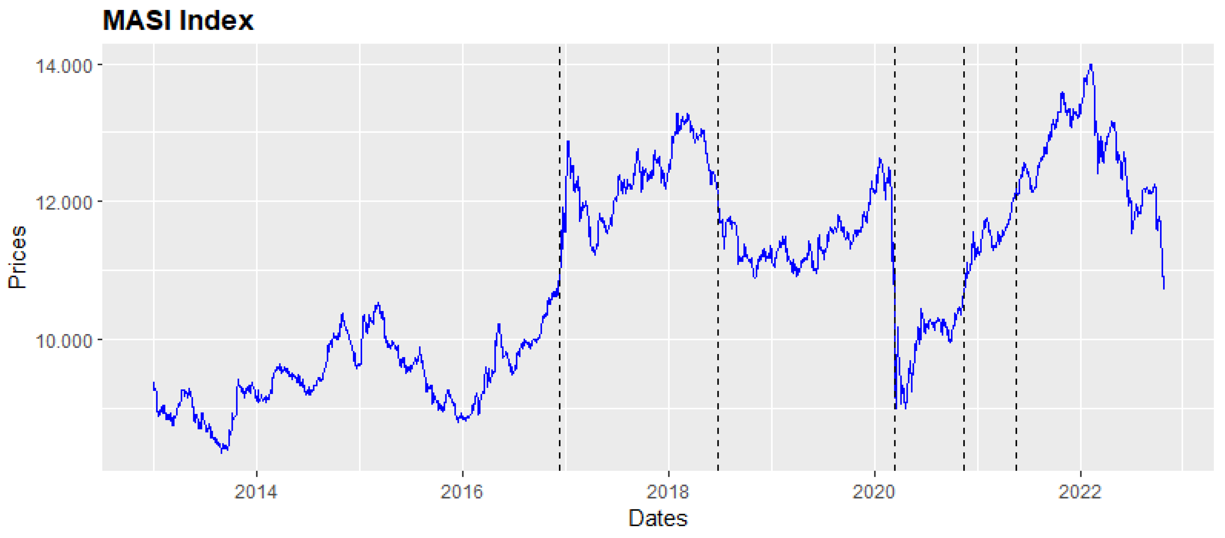
Before deep diving into analyses, it is crucial to better understand the studied market. The MSE market is recognized for its tendency towards high volatility and instability over short timeframes. In this market, prices can experience sudden and substantial fluctuations that may persist for extended periods. The MASI index serves as a clear indicator of this volatility, as it is subject to significant and rapid changes. This high level of fluctuation has had an impact on investors’ decisions, making them more uncertain and concerned about the security of the financial market. The market has seen a significant change in recent years, with many institutional investors who dominate the market adopting a strategy of holding onto their shares and waiting for market conditions to improve before investing. Since the 1993 reform, different stocks have begun to grow steadily. Moreover, Morocco has inaugurated new platforms which have been acquired by the CSE to strengthen market development and restore liquidity. Indeed, stagnating investment spending and falling trade levels are the main factors behind the liquidity crunch in the Moroccan market. Recently, the structure of the stock market has been improving over time. With the market becoming more integrated with the global economy, numerous groups of analysts and sources, such as S&P and Dow Jones, have started to recognize Morocco as one of the top-performing markets. Despite the impact of various crises worldwide, the COVID-19 pandemic has affected the MSE market, leading to a significant decline in revenue for several listed companies.
Despite the impact of various crises worldwide, the COVID-19 pandemic has affected the MSE market, leading to a significant decline in revenue for several listed companies. Following the emergence of early cases in the country, it is very easy to see how the overall market performance has declined since the first cases of coronavirus were reported domestically, starting 2 March 2020. The MASI index experienced a significant deterioration as a result of slower investment growth, losing about 26 per cent in April 2020 which is the lowest level in the last five years. The COVID-19 pandemic has affected companies listed on the MSE market in various ways. While some industries have shown resilience to the crisis, others have been significantly impacted. The uncertain future of the local economy and the financial situation of individuals has led to increased fear among investors, resulting in greater risks and reduced investment incentives. As a result, individuals and institutions started selling their stocks after the pandemic hit, causing a widespread decline in equity prices and value. Because of the low level of investment and the lofty level of ambiguity around the question of the crisis, the Moroccan economy has faced challenges. Consequently, the GDP indicator was significantly affected and several macroeconomic variables were influenced. However, the MASI index has started to recover from the immense impact of the crisis since October 2020. The evolution of several companies in the insurance, distribution, and real-estate sectors contributed in some manner to the progressive market recovery. Worldwide, global instability has various consequences, so investment analysts said that financial markets are heading into a major recession. Thereafter, the CSE market collapsed in 2022 after the invasion of Ukraine by Russia, causing a global stock market crash, soaring commodities, and strong demand on safe havens. The MASI widened its losses to end down 4.11 per cent, while The Moroccan Stock Index 20 (MSI20) dropped 4.54 per cent, which has created anxiety and uncertainty among investors.
The uncertainty pushes investors to develop and use efficient methods for portfolio optimization, to achieve good performance and robust portfolios. This article investigates the portfolio optimization stages: asset selection and allocation based on the MST method rather than traditional statistical methods. In this respect, the MST method was used for the stock selection and allocation based on the information extracted from historical stock returns. The choice of using this network method was based on the fact that it is one of the most used and performing models. In this paper, the stock price time series have been broken down into sub-periods based on structural change tests. In this respect, the Multiple Break Point Tests (MBPT)
Bai and Perron (
2003) was used to divide the MASI index time series. The results indicated that there were five structural changes in the MSE market (
Figure 1). Therefore, these results were used to divide the stock price time series into sub-periods; i.e., from the five resulting breaks with their corresponding dates—1: 9 December 2016, 2: 29 June 2018, 3: 12 March 2020, 4: 17 July 2020, and 5: 17 November 2021—we obtained six sub-periods, from SP1: sub-period1 to SB6: sub-period6 (
Figure 1), noting that the third break corresponding to the COVID-19 crisis is represented by a remarkable fall.
2.2. Methodology
This article aims to use the MST method and shows its relevance by applying it to the topic of portfolio optimization using MASI index. One must construct the MST structure, with the elements in the set defined according to the Gower distance metric using Prim’s algorithm. In addition, once the MST graph is obtained, centrality measures are calculated for better understanding the interrelations between stocks, and then we proceed to the stock selection and allocation stages. For the stock selection, we used two methods; the first one consists of the use of 63 stocks and the second one is based on the DC measure. In addition, the allocation result is obtained using the IDCP measure by extracting the weights. For portfolio construction, one must use two suggested portfolios. Starting with the MST-Portfolio, the asset selection is based on the 63 existing stocks and the allocation stage is based on the IDCP. Moreover, the second suggested portfolio is the MST-Portfolio 2, established using the DC measure for portfolio selection given 32 stocks with lower DC values, and the asset allocation process is given by the IDCP as an allocation method based on weights inverse to asset centrality. Knowing that, this method allocates a higher weight to peripheral assets in the network and therefore tries to establish a robust diversification and aims to prevent a fast spread of financial stress over the portfolio. The node representation variations, the structure of the network, and the definition of the distance allow different measures of potential risk to be applied. Risks can be calculated using methods such as centrality, assortativity, or others.
The aim of this paper lies in the use of the MST for portfolio optimization and showing its relevance. One must proceed to the construction of portfolios, EW Portfolio, MV Portfolio, and Rebalanced Portfolio, to compare them with the proposed portfolios which are the MST-Portfolio and MST-Portfolio 2, in order to evaluate their performances. The comparison between them required the use of some measures such as the Sharpe Ratio and Maximum Drawdown. Using empirical backtesting, we showed that the proposed network-based allocation concepts can help to improve the performance, the risk–return characteristic, and the diversification of a portfolio. MST network can be useful to add complementary information to the network and improve specific measures such as skewness or tail risk.
3. Results
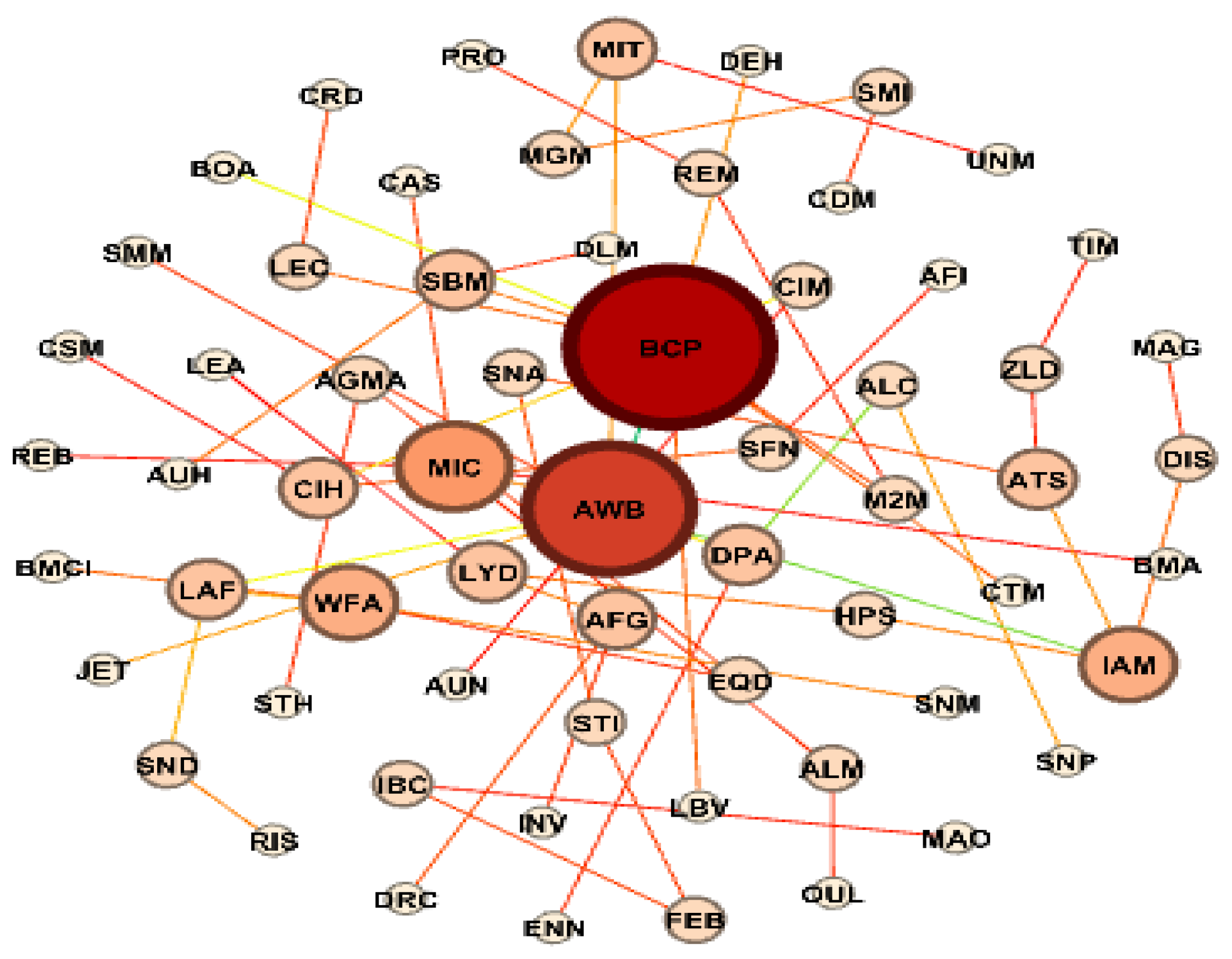
Figure 2 shows the obtained MST graph that connects all the stocks without forming any cycles, with a minimized size of the tree. Using this graph, and for a deeper understanding of the interconnections between stocks in the MSE market, centrality measures are used.
Focusing on the importance of every stock in the network,
Table 1 reports the rankings of stocks according to their network indicators; starting with the DC and Eigenvector Centrality (EC) of a node within a network, they take into account both the influence of the node and the importance of its neighbors in determining its overall impact. In this network, the BCP, AWB, and MIC stocks have a high degree of connectivity to numerous other stocks, making them among the most influential in the network. The Closeness Centrality (CC), AWB, CIH, and IAM stocks are the best positioned to quickly influence the entire network (
Rochat 2009). In addition, Betweenness Centrality (BC) demonstrates that AWB, BCP, and IAM stocks serve as a bridge between all nodes within the network. Moreover, HUBS and AUTHORITIES show that AWB, CIH, and M2M stocks acquire higher ranks, which means that the centrality value of these stocks acquire a high ability to form a relation with other stocks.
In this paper, we proceeded to the construction of three portfolios which are the MV Portfolio, EW Portfolio and finally the Rebalanced portfolio to compare them with the two proposed portfolios according to the proposed approach which are the MST-Portfolio and MST-Portfolio 2. The comparison between them was done at first sight using some measures to assess their performance and robustness.
According to practical considerations, the chosen portfolios for comparison are commonly used by researchers and investors, and have a significant market presence. This can make our analysis more relevant and practical for investors and other stakeholders. The reason why these three portfolios were chosen for portfolio performance comparisons are relative to some objective reasons that support our choice. These objective reasons include the relevance to our research objective to construct optimal portfolios with good performance. In terms of diversity, the chosen three portfolios are diverse in terms of their asset allocation and risk profile. This can help us to evaluate the effectiveness of the MST method in identifying the most efficient portfolios across different investment strategies. Moreover, the comparison with benchmark portfolios are commonly used as benchmarks for similar analyses, noting that EWPs can be a good benchmark for comparing the performance of other portfolios. By equally weighting all the assets in the portfolio, an EWP provides a simple and transparent approach to constructing a diversified portfolio. It also avoids the problem of overweighting a few large stocks, which can skew the portfolio’s performance.
DeMiguel et al. (
2009) compares the performance of the 1/N portfolio, which is an EWP, with the mean-variance efficient portfolios, and finds that the 1/N portfolio is not significantly worse than the mean-variance portfolios in terms of risk and return, suggesting that EWP can be a useful benchmark for portfolio comparison. In addition, MV Portfolios are designed to minimize the portfolio’s volatility or risk. This makes them a good benchmark for comparing the risk-adjusted performance of other portfolios. By constructing a portfolio that is highly diversified and has low correlations between assets, the MVP can provide a stable and predictable performance.
Clarke et al. (
2014) provides a comprehensive and detailed analysis of MV Portfolio strategies and examines its performance relative to traditional market capitalization-weighted portfolios, and finds that MV portfolios can provide superior risk-adjusted returns, suggesting that MV Portfolios can be a useful benchmark for portfolio comparison. Moreover, Rebalanced Portfolios can be a good benchmark for comparing the impact of different rebalancing frequencies or strategies. By adjusting the portfolio weights periodically, a rebalanced portfolio can maintain the desired asset allocation and reduce the portfolio’s risk. The frequency and timing of rebalancing can have a significant impact on the portfolio’s performance and risk (
Dichtl et al. 2016). These studies provide evidence for the use of EWP, MV Portfolios, and Rebalanced Portfolios in portfolio performance comparison and can provide useful benchmarks for evaluating portfolio performance. Comparing the performance of the two suggested portfolios to the MV Portfolio and EWP can provide insights into the added value of the optimization approach, which provide a reference point for evaluating the performance of the two suggested portfolios MST-Portfolio and MST-Portfolio 2.
By computing the Sharpe ratio, as represented in
Table 2, one may conclude that the best portfolios among the four are the suggested MST-Portfolio 2 and MST-Portfolio. Considering the CVaR of −0.0167, the MST-Portfolio 2 has the highest Sharpe ratio (0.5887) which means it is the one for which the investor will receive the highest excess return for the additional risk he or she will take, whereas the MST-Portfolio has a Sharpe ratio equivalent to 0.2828 and a CVaR of −0.0193. Consequently, for an investor indifferent about the difference in risk level, the first portfolio represents a very profitable investment option.
MST-Portfolio and MST-Portfolio 2 show the best performance of the Sharpe and Sortino ratios, followed by the EW Portfolio and MV Portfolio, noting that the MV Portfolio shows the worst performance. MST-Portfolio shows the lowest Maximum Drawdown, followed by the MST-Portfolio 2. Regarding the Skewness, the choice corresponds with the investor profile; if, for example, it is a conservative investor, a positive Skewness is preferable, noting that the highest Skewness referred to the MV Portfolio, followed by the MST-Portfolio 2 and MST-Portfolio. In addition, the lowest value of Kurtosis is returned for the MST-Portfolio 2, and the highest one is returned for the MST-Portfolio. As shown before, to assess how risky the portfolio is, the CVaR was computed using a 95-per cent confidence level, showing that the quantification of the tail risk amount for both MST-Portfolio and MST-Portfolio 2 are, respectively, −0.0193 and −0.0167, as the expected loss, and they acquire the smallest values of Maximum Drawdown.
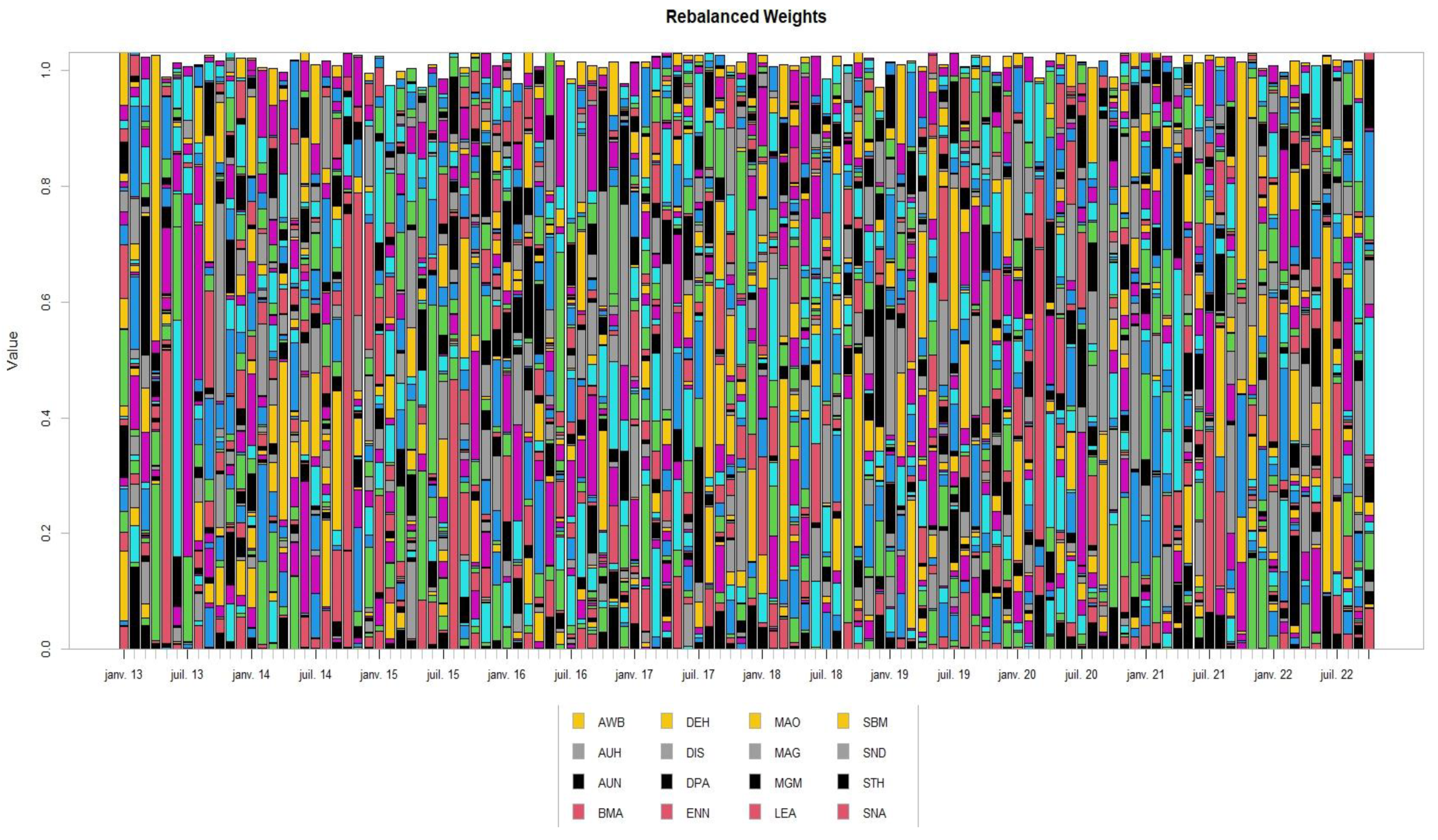
For a better understanding of the robustness of the rebalancing results, one must analyze the allocation method on an additional dataset of 10,000 scenarios generated using block bootstrapping. This helps to better assess the significance of the backtesting and to understand how much the results are driven by randomness or the choice of the asset universe. To do that, one must build blocks with a fixed length of 1 month and a random starting point in time based on the stock returns time series with a rolling window of 10 months. The scenarios are built by sampling the blocks with the replacement to rebuild a time series with the same length as the original time series. For these scenarios, we then calculated the resulting portfolio time series and the performance measures of the Rebalanced Portfolio compared to other portfolios.
Figure 3 shows the rebalanced weights for asset allocation during a particular time. For the purpose of simplification, only 16 stocks are presented in the legend, where the colors represent the 63 stocks. One must notice that the portfolio is well-diversified. There are several measures aiming to quantify the degree of diversification and to prove it. The most common ones are the Diversification Ratio (DR), Diversification Delta (DD), Diversification Delta Star (DD*), and Marginal Risk Contributions (MRC).
Table 3 shows that the MST-Portfolio gives good diversified risk budgets, and therefore exhibits the highest values. By construction, MST-Portfolio maximizes the diversification ratio. Regarding the other diversification metrics, one must consider that the suggested MST-Portfolio and MST-Portfolio 2 are well-diversified.
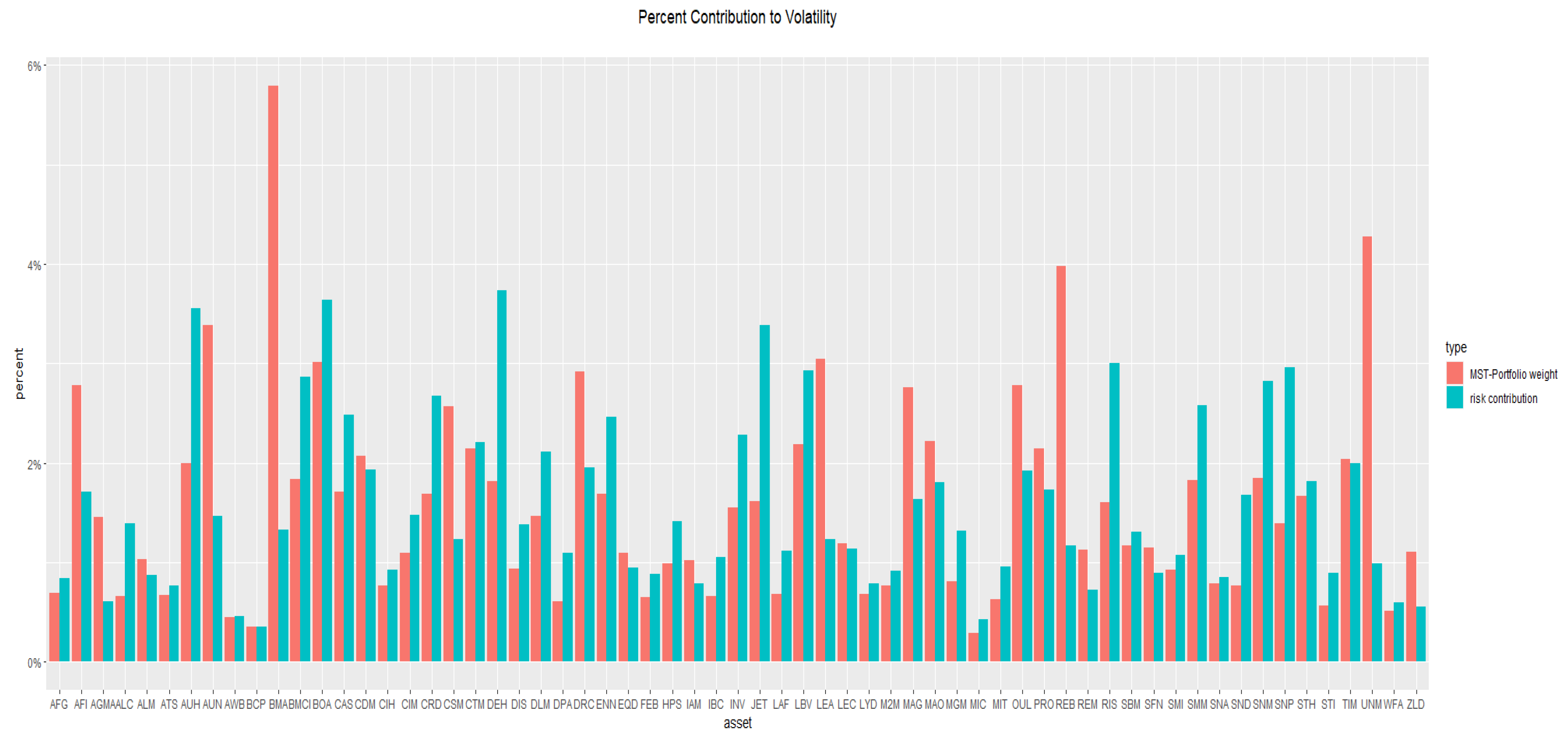
Table 4 represents the stock weights making up the MST-Portfolio as well as the risk contribution of each share to the portfolio risk. Based on
Figure 4, the x-axis represents the selected stocks in the MST-Portfolio with the following labels: AFI, AFG, AGMA, ALC, ALM, ATS, AWB, AUH, AUN, BMA, BOA, BCP, BMCI, CAS, CDM, CIH, CIM, CRD, CSM, CTM, DRC, DLM, DEH, DIS, DPA, ENN, EQD, FEB, HPS, IBC, INV, IAM, JET, LBV, LAF, LEC, LYD, M2M, MAO, MAG, MGM, LEA, MIC, MIT, OUL, PRO, REM, REB, RIS, SMM, SFN, SNM, SMI, SNP, SBM, SND, STH, SNA, STI, TIM, UNM, WFA, and ZLD. It can be pointed out that the greatest risk contribution is that of the DEH stock, followed by the BOA and AUH stocks. Otherwise, the smallest risk contribution goes to the BCP stock, followed by MIC and AWB, knowing that these stocks had a minimum weight.
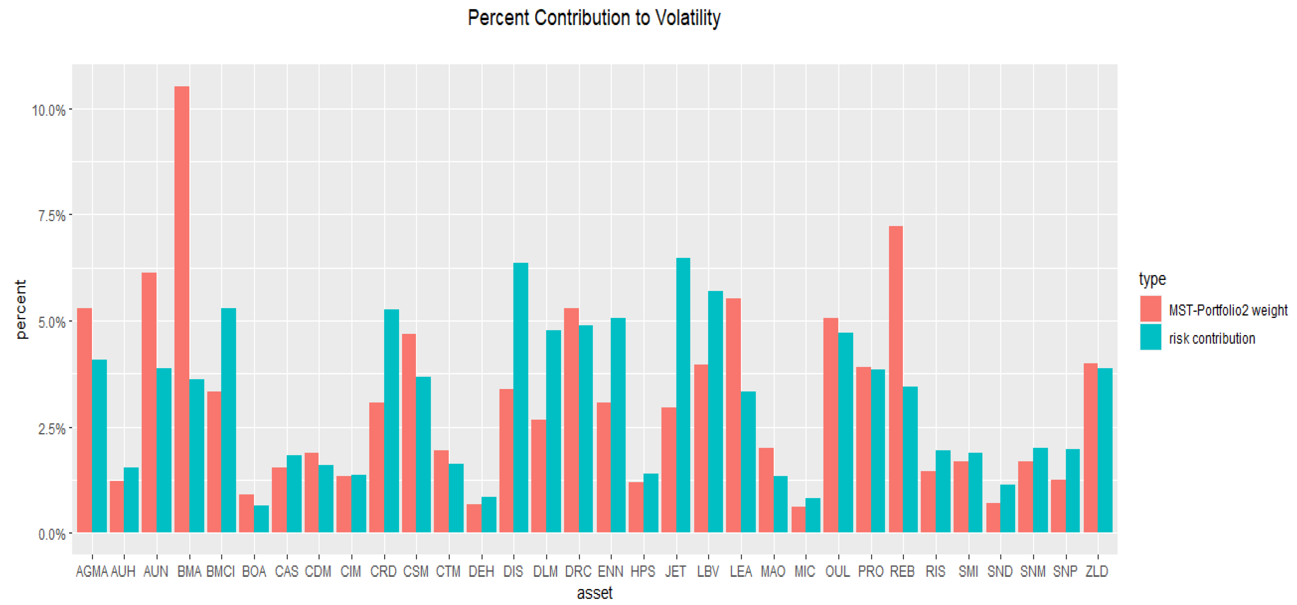
Table 5 shows the weights and the risk contribution of each stock constituting the MST-Portfolio 2 to the risk of the portfolio.
Figure 5 gives a visualization of the weights/risk contribution which allows us to say that the largest risk contribution to the MST-Portfolio 2 volatility has been the JET stock, which contributed by 0.0648 to portfolio volatility with a corresponding weight of 0.0294, followed by the DIS and BMCI stocks. On the other hand, the smallest risk contribution corresponds to the BOA stock, followed by the MIC and DEH stocks. It looks like the BOA stock has done a good job as a volatility dampener; it has a 0.00910 allocation but weakly contributes by 0.00639 to volatility. In addition, it can be deduced that 15 stocks out of 32 had a lower risk contribution than their corresponding weights in the MST-Portfolio 2, noting that the x-axis represents the selected stocks in the MST-Portfolio 2, with the following labels: AGMA, AUH, AUN, BMA, BOA, BMCI, CAS, CDM, CIM, CRD, CSM, CTM, DRC, DLM, DEH, DIS, ENN, HPS, JET, LBV, MAO, LEA, MIC, OUL, PRO, REB, RIS, SNM, SMI, SNP, SND, and ZLD.
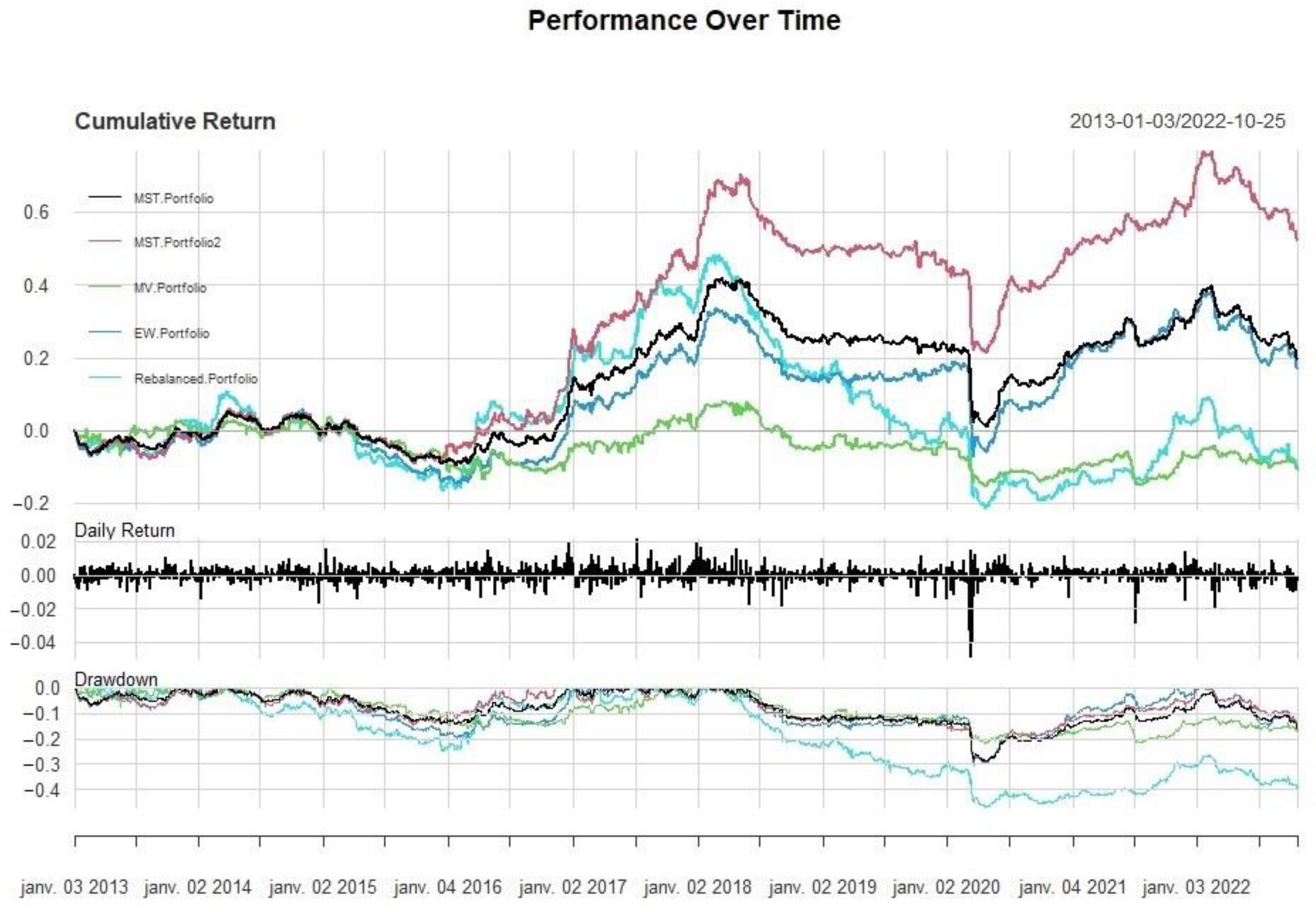
Figure 6 shows the performance and drawdowns of the MV Portfolio, EW Portfolio, Rebalanced Portfolio and the two suggested portfolios: MST-Portfolio and MST-Portfolio 2. Starting from 2017, the MST-Portfolio 2 has the highest cumulative returns, while the EW Portfolio is less volatile than the other portfolios. The MST-Portfolio seems like a balance between the MV Portfolio and MST-Portfolio 2. Furthermore, the EW Portfolio seems an interesting one here since both its return and volatility are acceptable, while it brings simplicity to the investment. The Rebalanced Portfolio shows a good trend relative to the cumulative returns until 2018; after this year, it had experienced a decline compared to the MST-Portfolio, which was able to keep an uptrend during this period. In addition, the MV Portfolio was able to absorb the fall that occurred during the COVID-19 crisis and the Rebalanced Portfolio underperforms the MST-Portfolio 2. The suggested strategy shows a remarkably good performance for the MST-Portfolio 2, but in the period prior to 2017, the suggested strategy performs rather poorly. According to
Bai and Perron (
2003) MBPT as shown in
Figure 1, this behavior is in line with
Bekaert and Harvey (
2002) studying the market finance, and the
Malagoli (
2016) paper concerning managing risk in institutional portfolios. By analyzing the performance over time, we notice that the MST-Portfolio and MST-Portfolio 2 show a good performance post-COVID-19 crisis—insights that can help investors and active managers when optimizing their portfolios.


